Epidemiological Dynamics of the 2009 Influenza A(H1N1)v Outbreak in India

Abstract

We analyze the time-series data for the onset of A(H1N1)v influenza pandemic in India during the period June 1- September 30, 2009. Using a variety of statistical fitting procedures, we obtain a robust estimate of the exponential growth rate $\langle\lambda\rangle\simeq 0.15$. This corresponds to a basic reproductive number $R_{0}\simeq 1.45$ for influenza A(H1N1)v in India, a value which lies towards the lower end of the range of values reported for different countries affected by the pandemic.

I Introduction

A novel influenza strain termed influenza A(H1N1)v, first identified in Mexico in March 2009, has rapidly spread to different countries and is currently the predominant influenza virus in circulation worldwide flu09 ; Jameel10 . As of April 11, 2010, it has caused at least 17798 deaths in 214 countries WHO10 . The first confirmed case in India, a passenger arriving from the USA, was detected on May 16, 2009 in Hyderabad. The initial cases were passengers arriving by international flights. However, towards the end of July, the infections appeared to have spread into the resident population with an increasing number of cases being reported for people who had not been abroad. As of 11 April 2010, there have been 30352 laboratory confirmed cases in India (out of 132796 tested) and 1472 deaths have been reported, i.e., $5~{}\%$ of the cases which tested positive for influenza A(H1N1)v MHO10 .

To devise effective strategies for combating the spread of pandemic influenza A(H1N1), it is essential to estimate the transmissibility of this disease in a reliable manner. This is generally characterized by the reproductive number $R$, defined as the average number of secondary infections resulting from a single (primary) infection. A special case is the basic reproductive number $R_{0}$, which is the value of $R$ measured when the overall population is susceptible to the infection as is the case at the initial stage of an epidemic. Estimate of the basic reproduction number for influenza A(H1N1)v in reports published from data obtained for different countries vary widely. For example, $R_{0}$ has been variously estimated to be between 2.2 to 3.0 for Mexico Boelle09 , 1.72 for Mexico City Cruz-Pacheco09 , between 1.4 and 1.6 for La Gloria in Mexico Fraser09 , between 1.3 to 1.7 for the United States Yang09 and 2.4 for Victoria State in Australia McBryde09 . The divergence in the estimates for the basic reproductive number may be a result of under-reporting in the early stages of the epidemic or due to climatic variations. They may also possibly reflect the effect of different control strategies used in different regions, ranging from social distancing such as school closures and confinement to antiviral treatments.

In this paper, we estimate the basic reproductive number for the infections using the time-series of infections in India extracted from reported data. By assuming an exponential rise in the number of infected cases $I(t)$ during the initial stage of the epidemic when most of the population is susceptible, we can express the basic reproductive number as $R_{0}=1+\lambda\tau$ (see, e.g., Ref. Anderson92 , p. 19), where $\lambda$ is the rate of exponential growth in the number of infections, and $\tau$ is the mean generation interval, which is approximately equal to 3 days Cruz-Pacheco09 . Using the time-series data we obtain the slope $\lambda$ of the exponential growth using several different statistical techniques. Our results show that this quantity has a value of around 0.15, corresponding to $R_{0}\simeq 1.45$.

II Methods

We used data from the daily situation updates available from the website of the Ministry of Health and Family Welfare, Government of India mohfw . In our analysis, data up to September 30, 2009 was used, corresponding to a total of 10078 positive cases. Note that, after September 30, 2009, patients exhibiting mild flu like symptoms (classified as categories A and B) were no longer tested for the presence of the influenza A(H1N1) virus.

As the data exhibit very large fluctuations, with some days not showing a single case while the following days show extremely large number of cases, it is necessary to smooth the data using a moving window average. We have used an $n$-day moving average ($n=2-10$), which removes large fluctuations while remaining faithful to the overall trend.

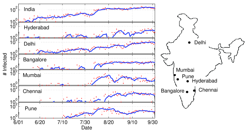
Figure 1: Time-series of the number of infected cases, $\#$Infected, of influenza A(H1N1)v showing the daily data (dotted) as well as the 5-day moving average (solid line) for India and the six metropolitan areas with the highest number of infections (whose geographic locations are shown in the adjoining map). The period shown is from June 1 to September 30, 2010. At the beginning of this period most of the infected people were arriving from abroad, while at the end of it the infection was entrenched in the local population. The data shows that almost all the cities showed a simultaneous increase in the number of infections towards the end of July and the beginning of August. This is manifested as a sudden rise in $\#$Infected for India as a whole (note the semilogarithmic scale), and can be taken as the period in which the infection started spreading in the resident population.

III Results

The incidence data for the 2009 pandemic influenza data in India immediately reveals that the disease has been largely confined to the urban areas of the country. Indeed, 6 of the 7 largest metropolitan areas of India (which together accommodate about 5 % of the Indian population worldgazetteer ) account for 7139 infected cases up to September 30, 2009, i.e., $70.8~{}\%$ of the data-set we have used.

Figure 1 shows the daily number of confirmed infected cases, as well as, the 5-day moving average from June 1 to September 30, 2009, for the country as a whole and the six major metropolitan areas which showed the highest incidence of the disease: Hyderabad, Delhi, Bangalore, Mumbai, Chennai and Pune. The adjoining map shows the geographic locations of these six cities. In the period up to July 2009, infections were largely reported in people arriving from abroad. There is a marked increase in the number of infections towards the end of July and the beginning of August 2009 in all of these cities (note that the ordinate is in logarithmic scale). This is manifest as a sudden rise in the number of infected cases for the country as a whole, implying that the infection started spreading in the resident population in the approximate period of 28 July to August 12.

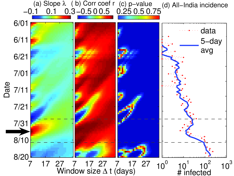
Figure 2: (a) The exponential slope $\lambda$ estimated from the time-series data of number of infected cases, $\#$Infected, averaged over a 5-day period to smoothen the fluctuations (d, solid curve). The slope $\lambda$ is calculated by considering the number of infected cases over a moving window having different sizes ($\Delta t$), ranging between 7 days and 36 days. By moving the starting point of the window across the period 1st June-20th August (in steps of 1 day) and calculating the best fit linear slope of the data on a semi-logarithmic scale (i.e., time in normal axis, number of infections in logarithmic axis) we obtain an estimate of $\lambda$. The arrow indicates the region between July 28-August 12 (region within the broken lines), which shows the largest increase in number of infections within the period under study, corresponding to the period when the epidemic broke out in the resident population. Over this time-interval, the average of $\lambda$ is calculated for the set of starting dates and window sizes over which (b) the correlation coefficient $r$ between log($\#$Infected) and $t$, is greater than $r_{cutoff}$ (we consider $0.75<r_{cutoff}<1$ in our analysis) and (c), the measure of significance for the correlation $p<0.01$.

Figure 2 (a) shows the exponential slope $\lambda$ estimated in the following way. The time-series of the number of infections is first smoothed by taking a 5-day moving average. The resulting smoothed time-series is then used to estimate $\lambda$ by a regression procedure applied to the logarithm of the number of infected cases [log($\#$infected)] across a moving window of length $\Delta t$ days. The origin of the window is varied across the period 1st June to 20th August (in steps of 1 day). We then repeat the procedure by varying the length of the window over the range of 7 days to 36 days. To quantify the quality of regression we calculate the correlation coefficient $r$ [Fig. 2 (b)] between log ($\#$Infected) and time (in days), and its measure of significance $p$ [Fig. 2 (c)]. The correlation coefficient $r$ is bounded between $-1$ and 1, with a value closer to 1 indicating a good fit of the data to an exponential increase in the number of infections. The measure of significance of the fitting is expressed by the corresponding $p$-value, which expresses the probability of obtaining the same correlation by random chance from uncorrelated data. The average of the estimated exponential slope $\lambda$ is obtained by taking the mean of all values of $\lambda$ obtained for windows originating between July 28-Aug 12 and of various sizes, for which the correlation coefficient $r>r_{cutoff}$ (we consider $0.75<r_{cutoff}<1$ in our analysis) and the measure of significance $p<0.01$. For comparison, we show again in Figure 2 (d) the number of infected cases of H1N1 in India (dotted) together with its 5-day moving average (solid line). The horizontal broken lines running across the figure indicate the period between July 28 and August 12 which exhibited the highest increase in number of infections within the period under study (from 1st June to 30th September) .

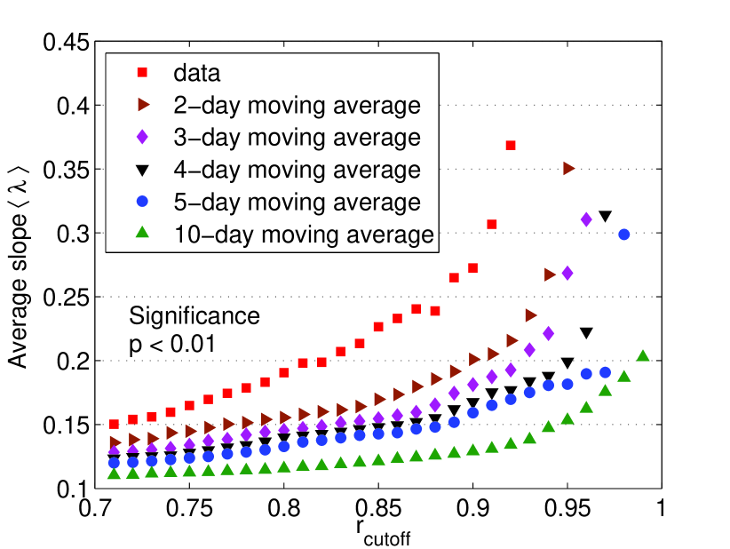
Figure 3: Average slope $\langle\lambda\rangle$ of the variation in log($\#$Infected) with time $t$, as a function of the threshold of correlation coefficient, $r_{cutoff}$, used to filter the data. The averaging is performed for infections occurring within the period July 28-August 12 (for details see caption to Fig. 2). Different symbols indicate the actual daily time-series data (squares) and the data smoothed over a moving $n$-day period, with $n$ = 2 (right-pointed triangle), 3 (diamond), 4 (inverted triangle), 5 (circle) and 10 (triangle). The significance of the correlation between log($\#$Infected) with time $t$, $p<0.01$ for all data points used in performing the average. Note that for $n=3,4,5$ the data show very similar profiles for variation of $\langle\lambda\rangle$ with $r_{cutoff}$, indicating the robustness of the estimate with respect to different values of $n$ used. The sudden increase in the value of the average slope around $r_{cutoff}\simeq 0.9$ implies that beyond this region the slope depends sensitively on the cutoff value. Considering the region where the variation is more gradual gives us an approximate value of the slope $\lambda\sim 0.15$, corresponding to a basic reproduction number $R_{0}\simeq 1.45$.

Figure 3 shows the average exponential slope $\langle\lambda\rangle$ as a function of $r_{cutoff}$, calculated for the original data and for different periods $n$ over which the moving average is taken ($n=2,3,4,5$ and 10). For $n=$ 3-5, the data show a similar profile indicating the robustness of the estimate of the average exponential slope $\langle\lambda\rangle$ with respect to different values of $n$. The sudden increase in $\langle\lambda\rangle$ around $r_{cutoff}\simeq 0.9$ implies that beyond this region the slope depends sensitively on the cutoff value. Considering the region where the variation is smoother gives an approximate value $\lambda\sim 0.15$, corresponding to a basic reproductive number for the epidemic $R_{0}=1+\lambda\tau\simeq 1.45$, assuming the mean generation interval, $\tau=3$ days.

We compute the confidence bounds for the estimate of $R_{0}$ from the 5-day moving average time-series by using the confint function of the scientific software MATLAB MATLAB . This function generates the goodness of fit statistics using the solution of the least squares fitting of log($\#$Infected) to a linear function. It results in a mean value $\langle\lambda\rangle=0.16$, with the corresponding $95~{}\%$ confidence intervals calculated as [0.116, 0.206], consistent with our previous estimate of $R_{0}\simeq 1.45$.

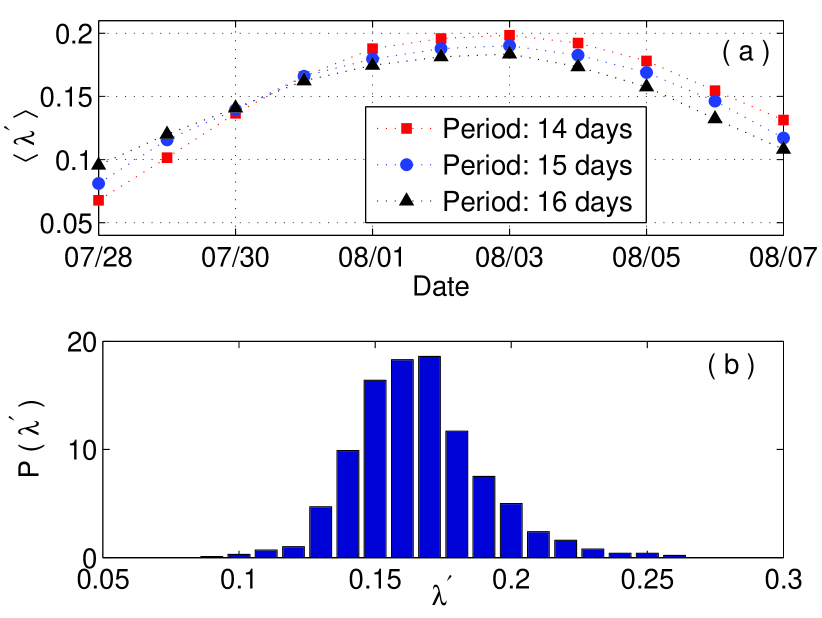
Figure 4: (a) The averages of the bootstrap estimates for the exponential slope, $\lambda^{\prime}$, calculated for different periods (with the abscissa indicating the starting date and the symbol indicating the duration) from the 5-day moving average time-series data of infected cases in India. The curves corresponding to the periods of different durations (14-16 days) intersect around July 31, 2010, indicating that the value of the average exponential slope is relatively robust with respect to the choice of the period about this date. (b) The distribution of bootstrap estimates of the exponential slope for the period July 31 to August 15, 2009. The average slope $\langle\lambda^{\prime}\rangle$ obtained from 1000 bootstrap samples is 0.166 with a standard deviation of 0.024, which agrees with the approximate value of $\lambda=0.15$ (corresponding to $R_{0}=1.45$) calculated in Fig. 3.

We have also used bootstrap methods to estimate the exponential slope, $\lambda$. This involves selecting random samples with replacement from the data such that the sample size equals the size of the actual data-set. The same analysis that was performed on the empirical data is then repeated on each of these samples. The range of the estimated values $\lambda^{\prime}$ calculated from the random samples allows determination of the uncertainty in estimation of $\lambda$. Fig. 4 (a) shows the average, $\langle\lambda^{\prime}\rangle$, calculated for different periods (with abscissa indicating the starting date and the symbol indicating the duration of the period) from the 5-day moving average time-series data of infected cases. The curves corresponding to the periods of different durations (14-16 days) intersect around July 31, 2010, indicating that the value of the average exponential slope is relatively robust with respect to the choice of the period about this date. The average value of the bootstrap estimates $\lambda^{\prime}$ at the intersection of the three curves is 0.15, in agreement with our earlier calculations of $\lambda$.

Fig. 4 (b) shows the distribution of the bootstrap estimates of the exponential slope for a particular period, July 31 to August 15, 2009. The average slope $\langle\lambda^{\prime}\rangle$ obtained from 1000 bootstrap samples for this period is 0.166 with a standard deviation of 0.024, which indicates that the spread of values around the average estimate of $\langle\lambda^{\prime}\rangle$ = 0.15 is not large. This confirms the reliability of the estimated value of the exponential slope, and hence of our calculation of the basic reproductive number.

IV Discussion

It may appear surprising that there was a very high number of infections in Pune (1238 positive cases up to September 30), despite it being less well-connected to the other major metropolitan cities of India, in comparison to urban centres that did not show a high incidence of the disease. For example, the Kolkata metropolitan area, which has a population around three times the population of the Pune metropolitan area worldgazetteer , had only 113 positive cases up to September 30. This could possibly reflect the role of local climatic conditions: Pune, located at a relatively higher altitude, has a generally cooler climate than most Indian cities. In addition, the close proximity of Pune to Mumbai and the high volume of road traffic between these two cities could have helped in the transmission of the disease. Another feature pointing to the role of local climate is the fact that in Chennai, most infected cases were visitors from outside the city, while in Pune, the majority of the cases were from the local population, even though the total number of infected cases listed for the two cities in our data-set are comparable (928 in Chennai and 1213 in Pune). This suggests the possibility that the incidence of the disease in Pune could have been aided by its cool climate, in contrast to the hotter climate of the coastal city of Chennai.

The calculation of $R_{0}$ for India assumes well-mixing of the population (i.e., homogeneity of the contact structure) among the major cities in India. Given the rapidity of travel between the different metropolitan areas via air and rail, this may not be an unreasonable assumption. However, some local variation in the development of the epidemic in different regions can indeed be seen (Fig. 1) . Around the end of July, almost all the cities under investigation showed a marked increase in the number of infected cases - indicating spread of the epidemic in the local population. This justifies our assumption of well-mixing in the urban population over the entire country for calculating the basic reproductive number.

To conclude, we stress the implications of our finding that the basic reproductive number for pandemic influenza A(H1N1)v in India lies towards the lower end of the values reported for other affected countries. This suggests that season-to-season and country-to-country variations need to be taken into account in order to formulate strategies for countering the spread of the disease. Evaluation of the reproductive number, once control measures have been initiated, is vital in determining the future pattern of spread of the disease.

Acknowledgements

We acknowledge the IMSc Complex Systems project and PRISM, IMSc for support.

References

-
(1)
2009 H1N1 Flu: International Situation Update, 22
January 2010. Available from:
http://www.cdc.gov/h1n1flu/updates/international - (2) Jameel, S., The 2009 influenza pandemic. Current Science, 2010, 98, 306-311.
-
(3)
World Health Organization, Pandemic (H1N1) 2009 -
update 96, 16 April 2010. Available from:
http://www.who.int/csr/don/2010_04_16/en/index.html -
(4)
Ministry of Health and Family Welfare, Government of
India, Situation Update on H1N1, 11 April 2010. Available from:
http://mohfw-h1n1.nic.in/documents/PDF/SituationalUpdatesArchives/april2010/Situational%20Updates%20on%2011.04.2010.pdf - (5) Boëlle, P. Y., Bernillon, P. and Desenclos, J. C., A preliminary estimation of the reproduction ratio for new influenza A(H1N1) from the outbreak in Mexico, March-April 2009. Euro Surveill., 2009, 14(19), pii: 19205.
- (6) Cruz-Pacheco, G., Duran, L., Esteva, L., Minzoni, A. A., Lopez-Cervantes, M., Panayotaros, P., Ahued Ortega, A. and Villasenor Ruiz, I., Modelling of the Influenza A(H1N1)v outbreak in Mexico City, April-May 2009, with control sanitary measures. Euro Surveill., 2009, 14(26), pii:19254.
- (7) Fraser, C., Donnelly, C. A., Cauchemez, S., Hanage, W. P., Van Kerkhove, M. D., Hollingsworth, T. D., Griffin, J., Baggaley, R. F., Jenkins, H. E., Lyons, E. J., Jombart, T., Hinsley, W. R., Grassly, N. C., Balloux, F., Ghani, A. C., Ferguson, N. M., Rambaut, A., Pybus, O. G., Lopez-Gatell, H., Alpuche-Aranda, C. M., Chapela, I. B., Zavala, E. P., Guevara, D. M., Checchi, F., Garcia, E., Hugonnet, S., Roth, C.; WHO Rapid Pandemic Assessment Collaboration, Pandemic potential of a strain of Influenza A(H1N1): Early findings. Science, 2009, 324 pp. 1557-1561.
- (8) Yang, Y., Sugimoto, J. D., Halloran, M. E., Basta, N. E., Chao, D. L., Matrajt, L., Potter, G., Kenah, E. and Longini, I. M., The transmissibility and control of pandemic influenza A(H1N1) virus. Science, 2009, 326, pp. 729-733.
- (9) McBryde, E., Bergeri, I., van Gemert, C., Rotty, J., Headley, E., Simpson, K., Lester, R., Hellard, M. and Fielding, J., Early transmission characteristics of influenza A(H1N1)v in Australia: Victorian state, 16 May - 3 June 2009. Euro Surveill., 2009, 14(42), pii: 19363.
- (10) Anderson, R. M. and May, R. M., Infectious Diseases Of Humans, Oxford University Press, Oxford, 1992.
-
(11)
http://mohfw-h1n1.nic.in/ -
(12)
http://www.world-gazetteer.com/(Retrieved on February 18, 2010) -
(13)
http://www.mathworks.com/