Factorization and resummation of s-channel single top quark production

Abstract:

We study the factorization and resummation of s-channel single top quark production in the Standard Model at both the Tevatron and the LHC. We show that the production cross section in the threshold limit can be factorized into a convolution of hard function, soft function and jet function via soft-collinear effective theory (SCET), and resummation can be performed using renormalization group equation in the momentum space resummation formalism. We find that the resummation effects significantly reduce the factorization scale dependence of the total cross section at the Tevatron, while at the LHC we find that the factorization scale dependence has not been improved, compared with the NLO results.

1 INTRODUCTION

Recently, the analysis of data by D0 [1] and CDF [2] collaboration has confirmed the observation of single top production at the Tevatron. Due to the fact that its expected production cross section is small ( in combined $s$ and $t$ channel, $\sigma_{st}\sim 2.9$ pb [3]) and the processes lack significant signal feature, such discovery signifies a success in both experiment and theory, and provides good opportunities for testing the Standard Model (SM) and searching for new physics.

As we know, at hadron collider, single top quarks are produced via three different modes: s-channel ($q\bar{q}^{\prime}\to\bar{b}t$), t-channel ($bq\to tq^{\prime}$ and $b\bar{q}\to t\bar{q}^{\prime}$), and associated $tW$ production ($bg\to tW^{-}$), each sensitive to quite different physics [4]. First of all, since all three production modes are directly proportional to the CKM matrix element $|V_{tb}|^{2}$, a measurement of the cross section provides a unique direct probe to $V_{tb}$, and can constrain models with fourth generation quark. The s-channel single top production is rather sensitive to the interaction mediated by extra heavy particle and the uncertainty of partonic luminosity for this mode is relatively small. Thus although this mode has the least cross section, it’s a very important channel in searching for new physics. The t-channel is sensitive to physics which modifies top decay properties, and the associated production channel can be a good measurement of the $W-t-b$ vertex. Thus a precise understanding of production cross sections and theoretical uncertainty are important. In particular, higher order QCD corrections to the cross section are necessary to improve theoretical predictions. There have been a lot of NLO calculations of the single top production in the literatures [5, 6, 7, 8, 3, 9, 10, 11, 12, 13, 14, 15, 16], with or without subsequent top quark decay. Recently, implementations of these results into NLO Shower Monte Carlo (MC@NLO or POWHEG) also appeared [17, 18, 19].

Furthermore, the consideration of phase space logarithms in higher order QCD effects, which origin from incomplete cancelation of real soft gluon emission and virtual corrections, are also important to the theoretical predictions. They often dominate the hadronic cross sections and can be systematically resummed to all orders in perturbation theory [20, 21]. For the single top production they have been calculated to NNLO at Next-to-next-to-Leading-Logarithmic (NNLL) accuracy [22, 23], but with some important NNLL logarithms omitted.

In recent years it has become popular to use SCET to resum the large phase space logarithms. SCET is an effective field theory describing the QCD interaction between collinear and soft particles [24, 25, 26, 27], which can correctly reproduce the long distance behavior of QCD, while the short distance information is encoded in the Wilson coefficients from matching the full theory to SCET. In the past decade, SCET has proved its usefulness in describing high energy hard scattering processes. These include deep-inelastic scattering [28, 29, 30, 31], Drell-Yan production [32, 33, 34, 35], Higgs production [36, 33, 37, 38, 39, 40], $e^{+}e^{-}$ annihilation to hadrons [41, 42, 43, 44, 45], color-octet scalar production [46], direct photon production [47], direct top quark production via FCNC coupling and top quark pair production [48, 49, 50, 51].

In this paper, we will further study the threshold resummation effects on the s-channel production cross section to all orders in QCD at NNLL accuracy in momentum space [30], utilizing SCET. First of all, we show that the total cross section for s-channel single top production can be factorized schematically as

$$\sigma=f\otimes f\otimes H\otimes S\otimes J,$$ (1)

where $f$ is the initial state nonperturbative parton distribution functions (PDFs); $H$ is the hard function, which encodes the short distance interaction information; $S$ is the soft function, which describes the soft correlation between different color objects; and $J$ is the jet function, describing the final state collinear emission associated with the jet. The factorized cross section we derived is valid in the hadronic threshold. In this limit, the partons initiated the hard scattering carry almost all of the hadron momentum, and the final state configuration consists of a top quark, a narrow hard jet and the remaining soft radiations. In this work, we are only intereseted in the inclusive total cross section, thus do not consider the top quark decay effects. For this reason, our results can not apply to the isolated s-channel single top cross section measured at the Tevatron, where explicit experimental cuts on the final state leptons and jets are required, but only serve as part of the total single top production cross section. When combined with the results of t-channel and $tW$ associated production channel, our results can provide the most accurate perturbative predictions for total cross section of single top production.

This paper is organized as follows. In Section 2, we briefly review the basic ingredients of SCET. Section 3 discusses the kinematics at threshold. In section 4 we derive a factorization formula for the resummed cross section in momentum space. We give a NNLO expansion of our resummed cross section in section 5. Section 6 contains a brief numerical discussion and we conclude at section 7.

2 Brief introduction to SCET

To describes collinear field in SCET, it is convenient to define a lightlike vector $n_{\mu}=(1,\mathbf{n}),\mathbf{n}^{2}=1$. Any four-vector can be decomposed with respect to $n_{\mu}$ and $\bar{n}_{\mu}=(1,-\mathbf{n})$ as

$$l^{\mu}=l^{-}\frac{n^{\mu}}{2}+l^{+}\frac{\bar{n}^{\mu}}{2}+l^{\mu}_{n\perp},$$ (2)

with $l^{+}=n\!\cdot\!l$ and $l^{-}=\bar{n}\!\cdot\!l$. The momentum of a collinear particle moving along the $n^{\mu}$ direction has the following scaling

$$p^{\mu}=(p^{+},p^{-},p_{n\perp})\sim(\lambda^{2},1,\lambda),$$ (3)

while for a soft particle, the momentum scales as

$$q\sim(\lambda^{2},\lambda^{2},\lambda^{2}),$$ (4)

where $\lambda\ll 1$ is a small expansion parameter in SCET. E.g., for an energetic jet with invariant mass $m_{J}$ and energy $E_{J}$, $\lambda=m_{J}/E_{J}$. From the momentum scaling, one can see that the interaction between collinear fields of different directions $n_{i}$ and $n_{j}$ with $n_{i}\cdot n_{j}\gg\lambda^{2}$ will inevitably change the momentum scaling, thus is forbidden in SCET, but can be included as an external current in our computation. The soft fields, on the other hand, can interact with any collinear field without changing the scaling.

A $n$-collinear quark and gluon field can be written as

$$\chi_{n}(x) = W^{\dagger}_{n}(x)\xi_{n}(x),$$

$$\mathcal{B}^{\mu}_{n\perp}(x) = \left[W^{\dagger}_{n}iD^{\mu}_{n\perp}W_{n}(x)\right],$$ (5)

where

$$iD^{\mu}_{n\perp}=\mathcal{P}^{\mu}_{n\perp}+g_{s}A^{\mu}_{n\perp}$$ (6)

is the collinear covariant derivative and the label operator $\cal P$ is defined to project out the large momentum component of the collinear field, e.g., ${\cal P}^{\mu}_{n}\xi_{n}=\bar{p}^{\mu}\xi_{n}$. Here we have split $p$ into a sum of large label momentum and small residue momentum,

$$p^{\mu}=\bar{p}^{\mu}+k^{\mu},\qquad\text{with}\qquad\bar{p}^{\mu}=p^{-}\frac{n^{\mu}}{2}+p^{\mu}_{n\perp}.$$ (7)

The collinear Wilson line,

$$W_{n}(x)=\mathbf{P}\exp\left(ig_{s}\int^{0}_{-\infty}ds\,{\bar{n}}\!\cdot\!A^{a}_{n}(x+s{\bar{n}})t^{a}\right),$$ (8)

which describes the emission of arbitrary $n$-collinear gluons from an $n$-collinear quark or gluon, is constructed to make the collinear fields as defined in Eq. (2) invariant under the collinear gauge transformation. The operator $\mathbf{P}$ is the path-ordered operator acting on the color generator $t^{a}$.

At the leading order in $\lambda$, only the $n\!\cdot\!A_{s}$ component of soft gluons can interact with the $n$-collinear field. Such interaction is Eikonal and can be removed by a field redefinition [27]:

$$\chi_{n}(x) = Y_{n}(x)\chi^{(0)}_{n}(x),$$

$$\mathcal{B}^{\mu}_{n\perp}(x) = Y_{n}(x)\mathcal{B}^{\mu(0)}_{n\perp}(x)Y^{\dagger}_{n}(x),$$ (9)

where

$$Y_{n}(x)=\mathbf{P}\exp\left(ig_{s}\int^{0}_{-\infty}ds\,n\!\cdot\!A^{a}_{s}(x+sn)t^{a}\right)$$ (10)

for an incoming Wilson line [52]. And for an out going Wilson line, it is defined as

$$\tilde{Y}_{n}(x)=\mathbf{P}\exp\left(-ig_{s}\int^{\infty}_{0}ds\,n\!\cdot\!A^{a}_{s}(x+sn)t^{a}\right).$$ (11)

The fields with superscript (0) now are decoupled with soft gluons. Without confusion, we will neglect the superscript below. After the field redefinition, the leading order SCET lagrangian is factorized into a sum of different collinear sectors and soft sector, which do not interact with each other,

$$\mathcal{L}_{\rm SCET}=\sum_{n_{i}}\mathcal{L}^{(0)}_{n_{i}}+\mathcal{L}_{s}+\cdots.$$ (12)

3 Analysis of kinematics

In this section, we introduce the relevant kinematical variables needed in our analysis. As an example, we consider the subprocess $u+\bar{d}\to t+X$. The subprocesses induced by gluon splitting are power suppressed in the threshold limit, therefore will not be considered in this paper. First of all, we define two lightlike vectors along the beam directions, $n_{a}$ and $n_{b}$, which are related by $n_{a}=\bar{n}_{b}$. Then we introduce initial collinear fields along $n_{a}$ and $n_{b}$ to describe the collinear particles in the beam directions. In the center-of-mass frame of the hadronic collision, the momentum of the incoming hadrons can be written as

$$P^{\mu}_{a}=E_{\rm CM}\frac{n^{\mu}_{a}}{2},\qquad P^{\mu}_{b}=E_{\rm CM}\frac{n^{\mu}_{b}}{2}.$$ (13)

Here $E_{\rm CM}$ is the center-of-mass energy of the collider and we have neglected the masses of the hadrons. The momentum of the incoming partons, with a light-cone momentum fraction of the hadronic momentum, are

$$\tilde{p}_{a}=x_{a}E_{\rm CM}\frac{n^{\mu}_{a}}{2},\qquad\tilde{p}_{b}=x_{b}E_{\rm CM}\frac{n^{\mu}_{b}}{2}.$$ (14)

At the hadronic and partonic level, momentum conservation means

$$P_{a}+P_{b}=q+P_{X},$$ (15)

and

$$\tilde{p}_{a}+\tilde{p}_{b}=q+p_{X},$$ (16)

respectively, where $q$ is the momenta of the top quark. We define the partonic jet with jet momentum $p_{X}$ to be the set of all final state partons except the top quark in the partonic processes, while the hadronic jet with jet momentum $P_{X}$ contains all the hadrons as well as the beam remnants in the final state, except the top quark. Explicitly, $p_{X}=p_{1}+k$, where $p_{1}$ is the momentum of the final state collinear partons forming the jet and $k$ is the momentum of the soft radiations. Such division of momentum is artificial and we have to integrate over the soft momentum to obtain a physical observable. We also define the Mandelstam variables as

$$s=(P_{a}+P_{b})^{2},\quad u=(P_{a}-q)^{2},\quad t=(P_{b}-q)^{2}$$ (17)

for hadrons, and

$$\hat{s}=(\tilde{p}_{a}+\tilde{p}_{b})^{2},\quad\hat{u}=(\tilde{p}_{a}-q)^{2},\quad\hat{t}=(\tilde{p}_{b}-q)^{2}$$ (18)

for partons, respectively. In terms of the Mandelstam variables, the hadronic and partonic threshold variables are defined as $S_{4}\equiv P^{2}_{X}=s+t+u-m^{2}_{t}$ and $s_{4}\equiv p^{2}_{X}=\hat{s}+\hat{t}+\hat{u}-m^{2}_{t}$, where $m_{t}$ is the mass of top quark. The hadronic threshold limit is defined as $S_{4}\to 0$ [53]. In this limit, the final state radiations and beam remnants are highly suppressed, leads to a configuration consists of a top quark and a narrow jet, as well as the remaining soft radiations. Taking this limit requires $x_{a}\to 1,\;x_{b}\to 1,\;s_{4}\to 0$ simultaneously. Thus, the hadronic threshold enforces the partonic threshold. However, the reverse is not true. The partonic threshold $s_{4}\to 0$ does not forbid a significant amount of beam remnants. We note that in both hadronic threshold limit and partonic threshold limit, the top quark is not forced to be produced at rest, $i.e.$ it can have a large momentum. For later convenience, we can also write the threshold variable as

$$s_{4}=p^{2}_{X}=(\tilde{p}_{a}+\tilde{p}_{b}-q)^{2}=p^{2}_{1}+2k^{+}E_{1}+{\cal O}(k^{2}),$$ (19)

where $k^{+}=n_{1}\!\cdot\!k$, $E_{1}$ is the energy of the quark jet and $n_{1}$ is the lightlike vector associated with the jet direction. Note that our definition of $s_{4}$ is different from [22], in which the definition $\bar{s}_{4}=(\tilde{p}_{a}+\tilde{p}_{b}-p_{1})^{2}-m^{2}_{t}$ is adopted, where we put a bar on $s_{4}$ to distinguish the definition in [22] from ours. We point out that the meaning of such choice is not clear, because $\bar{s}_{4}$ doesn’t vanish when there are collinear gluon emitting from the final state b-quark. However, as we know, there are large logarithms associated with such collinear gluon emission, thus, the definition adopted in [22] could miss some large contributions.

In the threshold limit ($s_{4}\to 0$), incomplete cancelation between real and virtual corrections leads to singular distributions $\alpha^{n}_{s}[\ln^{m}(s_{4}/m^{2}_{t})/s_{4}]_{+}$, with $m\leq 2n-1$. It is the purpose of threshold resummation to sum up these contributions to all orders in perturbation theory.

4 Factorization in SCET

In this section, we derive the factorized cross section formula for s-channel single top production in SCET, following the convention and formalism of [54, 55]. With appropriate changes, our formula can be extended to the resummation of t-channel and $tW$ associated production channel as well, which will be presented elsewhere [wang, 57].

Total cross section for s-channel single top production can be written as [54]:

$$\sigma = \frac{1}{2E^{2}_{\rm CM}}\sum^{\rm res.}_{X}\langle I|O^{\dagger}_{x}(0)|X\rangle\langle X|O_{x}(0)|I\rangle(2\pi)^{4}\delta^{4}(P_{a}+P_{b}-p_{X})$$ (20)

$$= \frac{1}{2E^{2}_{\rm CM}}\sum^{\rm res.}_{X}\int d^{4}x\langle I|O^{\dagger}_{x}(x)|X\rangle\langle X|O_{x}(0)|I\rangle$$

$$= \frac{1}{2E^{2}_{\rm CM}}\sum^{\rm res.}_{X}\int d^{4}x\int\frac{d^{4}k}{(2\pi)^{4}}e^{-ik\cdot x}\int\frac{d^{4}p}{(2\pi)^{4}}\langle I|O^{\dagger}(k)|X\rangle\langle X|O(p)|I\rangle$$

$$= \frac{1}{2E^{2}_{\rm CM}}\sum^{\rm res.}_{X}\int\,\frac{d^{4}p}{(2\pi)^{4}}\langle I|O^{\dagger}(0)|X\rangle\langle X|O(p)|I\rangle,$$

where $|I\rangle=|P_{a}P_{b}\rangle$ denotes the initial state protons (anti-protons), $O_{x}(x)$ is the relevant operator responsible for the underlying hard interaction, and $O(p)$ its fourier transformation. Here we distinguish the position space operator from the momentum space one by a subscript $x$. The restriction on the sum over final states $|X\rangle$ is that we include final state configuration consists only of a top quark jet whose 3-momentum is in the direction of $\bar{n}_{1}$, an anti b quark quark jet in the direction of $n_{1}$, and soft radiations. This is the configuration that is relevant to threshold resummation and we are interested in. Under this condition the final state can be written as $|X\rangle=|X_{t}X_{1}X_{s}\rangle$, where $|X_{t}\rangle$, $|X_{1}\rangle$ and $|X_{s}\rangle$ denote top quark jet, anti b quark jet and remaining soft radiations, respectively. In the second line of Eq. (20), we have used the momentum conservation delta function to shift the operator $O_{x}^{\dagger}$ to point $x$, and in the third line written the operators in momentum space, which are then matched onto SCET operators. We chose to match directly in momentum space, which has the advantage that the cumbersome label summations and residual soft integration can be combined to a full four momentum integral [54]. After matching we obtain

$$O(p) = \int\,\frac{d^{4}p_{a}}{(2\pi)^{4}}\frac{d^{4}p_{b}}{(2\pi)^{4}}\frac{d^{4}p_{1}}{(2\pi)^{4}}\frac{d^{4}p_{2}}{(2\pi)^{4}}\frac{d^{4}k_{s}}{(2\pi)^{4}}\mathcal{C}_{I}(p_{a},p_{b};p_{1},p_{2})$$ (21)

$$\times{\cal O}_{in}(p_{a},p_{b}){\cal O}_{out}(p_{1},p_{2}){\cal O}_{S,I}(k_{s})(2\pi)^{4}\delta^{(4)}(p-p_{a}-p_{b}+p_{1}+p_{2}+k_{s}).$$

In the above equation, we have made all the spin, Lorentz and color indices implicit. For example, at the LO, the hard matching coefficient $\mathcal{C}_{I}$ reads

$$\mathcal{C}_{I}=i\frac{\alpha\pi V^{*}_{ud}V_{tb}}{2\sin^{2}\theta_{W}((p_{a}+p_{b})^{2}-M^{2}_{W})}(\gamma^{\mu}(1-\gamma^{5}))^{\gamma\delta}(\gamma_{\mu}(1-\gamma^{5}))^{\alpha\beta}\delta_{I1},$$ (22)

where $\alpha$ is the fine-structure constant, $V_{ij}$ the CKM matrix element, $\theta_{W}$ the electroweak mixing angle, and $M_{W}$ the mass of the $W$ boson. Here we have chosen the s-channel singlet-octet basis as the independent color structure for this process:

$$|c_{1}\rangle=\delta_{cd}\delta_{ef},\qquad|c_{2}\rangle=(t^{a})_{cd}(t^{a})_{ef},$$ (23)

and $I=1$ or $2$ is an index in this color space. Thus the kronecker delta function in Eq. (22) can be understood that at the LO the final state $t\bar{b}$ pair of s-channel single top production is a color-singlet. In Eq. (21) $\mathcal{O}_{in}$ denotes the effective operator responsible for annihilating an initial state collinear up-type quark with momentum $p_{a}$ and an down-type anti-quark with momentum $p_{b}$, which can be written as

$${\cal O}^{cd}_{\alpha\beta,in}=\bar{\chi}^{c}_{\alpha}(-p_{b})\chi^{d}_{\beta}(p_{a}),$$ (24)

and $\mathcal{O}_{out}$ is the effective operator responsible for the creation of final state anti-bottom quark with momentum $p_{1}$ and top quark with momentum $p_{2}$, which can be expressed as

$${\cal O}^{ef}_{\gamma\delta,out}=\bar{h}^{e}_{\gamma,v}(p_{2})\chi^{f}_{\delta}(-p_{1}).$$ (25)

Note that we have taken the $m_{t}\to\infty$ limit at fixed top jet radius and then described the top quark in terms of the heavy quark effective field [58] with label velocity $v$. The fields in Eqs. (24) and (25) are defined with field redefinition in Eq. (2), thus they no longer interact with soft degrees of freedom.

The soft operators ${\cal O}_{S,I}$, which are responsible for the soft interactions between different collinear sectors and top quark, are expressed as

$${\cal O}_{S,1}(k_{s}) = \int\,d^{4}xe^{-ik_{s}\,\!\cdot\!\,x}\mathbf{T}\left[\left(Y^{\dagger}_{n_{b}}(x)Y_{n_{a}}(x)\right)^{cd}\left(\tilde{Y}^{\dagger}_{v_{2}}(x)\tilde{Y}_{n_{1}}(x)\right)^{ef}\right],$$

$${\cal O}_{S,2}(k_{s}) = \int\,d^{4}xe^{-ik_{s}\,\!\cdot\!\,x}\mathbf{T}\left[\left(Y^{\dagger}_{n_{b}}(x)t^{a}Y_{n_{a}}(x)\right)^{cd}\left(\tilde{Y}^{\dagger}_{v_{2}}(x)t^{a}\tilde{Y}_{n_{1}}(x)\right)^{ef}\right],$$ (26)

where the time-ordering operator $\mathbf{T}$ is required to ensure the proper ordering of soft gluon fields in the soft Wilson line.

Using the notation $\Phi_{2}=\{p_{a},p_{b};p_{1},p_{2}\}$ to express a phase space point [54] with $d\Phi_{2}=d^{4}p_{a}d^{4}p_{b}d^{4}p_{1}d^{4}p_{2}/(2\pi)^{16}$ and $\Phi_{2}-k_{s}=p_{a}+p_{b}-p_{1}-p_{2}-k_{s}$, we can write Eq. (20) in a compact form

$$\sigma = \frac{1}{2E^{2}_{\rm CM}}\sum^{res}_{X}\int d\Phi^{\prime}_{2}d\Phi_{2}\mathcal{C}^{*}_{J}(\Phi^{\prime}_{2})\mathcal{C}_{I}(\Phi_{2})\int\frac{d^{4}k^{\prime}_{s}}{(2\pi)^{4}}\,\frac{d^{4}k_{s}}{(2\pi)^{4}}(2\pi)^{4}\delta^{(4)}(\Phi_{2}-k_{s})$$ (27)

$$\times\langle I|({\cal O}^{\prime}_{in}{\cal O}^{\prime}_{out}{\cal O}^{\prime}_{S,J})^{\dagger}|X_{t}X_{1}X_{s}\rangle\langle X_{t}X_{1}X_{s}|({\cal O}_{in}{\cal O}_{out}{\cal O}_{S,I})|I\rangle.$$

As we mentioned before, different collinear sectors are decoupled due to field redefinition, and thus the matrix element in Eq. (27) can be factorized into a product of several matrix elements, which obey certain renormalization group (RG) equation.

In the following, we further show the matrix elements mentioned above. First, we deal with the top quark sector. Since we have decoupled the soft interaction by field redefinition, the top quark now should be regarded as a non-interacting particle, which can be written as

$$\sum_{X_{t}}\int\frac{d^{4}p^{\prime}_{2}}{(2\pi)^{4}}\frac{d^{4}p_{2}}{(2\pi)^{4}}\langle 0|{h^{e^{\prime}}_{\gamma^{\prime},v^{\prime}_{2}}}(p^{\prime}_{2})|X_{t}\rangle\langle X_{t}|\bar{h}^{e}_{\gamma,v_{2}}(p_{2})|0\rangle...$$

$$= \int\frac{d^{3}q}{2E_{q}(2\pi)^{3}}({q\!\!\!/}+m_{t})_{\gamma^{\prime}\gamma}\delta_{e^{\prime}e}...$$ (28)

where summation over final state $|X_{t}\rangle$ gives rise to a top quark phase space integral. Next, we define the soft function by the soft matrix element as

$$S^{f^{\prime}e^{\prime}d^{\prime}c^{\prime}cdef}_{JI}(k^{+},\mu) = \sum_{X_{s}}\int dk^{+}\frac{d^{4}k^{\prime}_{s}}{(2\pi)^{4}}\frac{d^{4}k_{s}}{(2\pi)^{4}}\langle 0|{\mathcal{O}^{\dagger,f^{\prime}e^{\prime}d^{\prime}c^{\prime}}_{S,J}}(k^{\prime}_{s})$$ (29)

$$\delta[k^{+}-n_{1}\!\cdot\!k_{s}]|X_{s}\rangle\langle X_{s}|\mathcal{O}^{cdef}_{S,I}(k_{s})|0\rangle,$$

where we have inserted into the above equation an identity operator

$$\mathbf{1}=\int dk^{+}\,\delta[k^{+}-n_{1}\!\cdot\!k_{s}].$$ (30)

Note that the summation over final state can be performed $\sum_{X_{s}}|X_{s}\rangle\langle X_{s}|=1$ since there is no restriction in the summation when written between the soft operator and also there is no explicit dependence on $|X_{s}\rangle$. Since we are only interested in the total cross sections, the final state top quark, jet function and PDFs can be considered to be diagonal in color space. Then we can contract them to obtain the soft function matrix

$$S_{JI}(k^{+},\mu)=\delta^{f^{\prime}f}\delta^{e^{\prime}e}\delta^{d^{\prime}d}\delta^{c^{\prime}c}S^{f^{\prime}e^{\prime}d^{\prime}c^{\prime}cdef}_{JI}(k^{+},\mu).$$ (31)

At the LO, it can be written as

$$\mathbf{S}(k^{+},\mu)=\delta(k^{+})\left(\begin{array}[]{cc}N^{2}_{c}&0\\ 0&\frac{N^{2}_{c}-1}{4}\end{array}\right).$$ (32)

At the NLO, the calculation of soft function boils down to the evaluation of eikonal diagrams [47]. Since the virtual corrections in SCET vanish, only real emission diagrams, which are shown in Figs. 1, are needed to be evaluated. The detail calculation of these diagrams are given in the appendix.

(a)	(b)	(c)
(d)	(e)	(f)
	(g)

Figure 1: Diagrams contribute to the soft function. the double line represents the top quark line. Diagrams (a), (c), (d), (e), (f) and (g) have their mirror image diagrams. There are also diagrams with soft gluon connecting to the same massless quark line on the two side of the cut, which are not shown here because they vanish identically. The cross dot in the diagrams represents either singlet or octet operator.

For the final state anti-quark jet sector, we have [54]

$$\sum_{X_{1}}\int\frac{d^{4}p^{\prime}_{1}}{(2\pi)^{4}}\frac{d^{4}p_{1}}{(2\pi)^{4}}\langle 0|\bar{\chi}^{f^{\prime}}_{\delta^{\prime}}(-p^{\prime}_{1})|X_{1}\rangle\langle X_{1}|\chi^{f}_{\delta}(-p_{1})|0\rangle$$

$$=\delta^{f^{\prime}f}\int\frac{d^{4}p_{1}}{(2\pi)^{3}}\left(\frac{{n\!\!\!/}_{1}}{2}\right)_{\delta\delta^{\prime}}\theta(p^{0}_{1})p^{-}_{1}J(p^{2}_{1}),$$ (33)

Again, summation over collinear state has been performed and $J$ is the spin and color singlet jet function, which can be defined as

$$\theta(p^{0})p^{-}J(p^{2})=\frac{1}{8\pi N_{c}}\int\frac{d^{4}p^{\prime}}{(2\pi)^{4}}{\rm Tr}\langle 0|\bar{\chi}(-p^{\prime})\bar{n}\!\!\!/_{1}\chi(-p)|0\rangle.$$ (34)

Finally, the initial state collinear sector reduces to the conventional PDFs [27], of which the matrix element for $n_{a}$ direction is

$$\int\frac{d^{4}p^{\prime}_{a}}{(2\pi)^{4}}\frac{d^{4}p_{a}}{(2\pi)^{4}}\langle P_{a}|\bar{\chi}^{d^{\prime}}_{\beta^{\prime}}(p^{\prime}_{a})\chi^{d}_{\beta}(p_{a})|P_{a}\rangle=\frac{1}{2N_{c}}\delta^{d^{\prime}d}\int^{1}_{0}\frac{dx_{a}}{x_{a}}\left(x_{a}E_{\rm CM}\frac{{n\!\!\!/}_{a}}{2}\right)_{\beta\beta^{\prime}}f(x_{a},\mu),$$ (35)

and similarly for the matrix element for $n_{b}$ direction. Thus the momentum of incoming partons are given by $\tilde{p}_{a,b}=x_{a,b}E_{\rm CM}n^{\mu}_{a,b}/2$.

Combining the above expressions, we obtain (up to power corrections)

$$\sigma = \frac{1}{2E^{2}_{\rm CM}}\frac{1}{4N^{2}_{c}}\int^{1}_{0}\frac{dx_{a}}{x_{a}}\frac{dx_{b}}{x_{b}}\int\frac{d^{3}q}{2E_{q}(2\pi)^{3}}f_{i/P_{a}}(x_{a},\mu_{f})f_{j/P_{b}}(x_{b},\mu_{f})\lambda_{0,ij}H_{IJ}$$ (36)

$$\times\int dk^{+}\,S_{JI}(k^{+}_{i},\mu)(2\pi)J(s_{4}-2k^{+}E_{1},\mu),$$

with

$$\lambda_{0,ij}=\frac{e^{4}}{\sin^{4}\theta_{W}}|V_{ij}|^{2}|V_{tb}|^{2}\frac{(\hat{t}-m^{2}_{t})\hat{t}}{(\hat{s}-M^{2}_{W})^{2}}.$$ (37)

At the LO, the hard function $H_{IJ}$ is normalized to $\delta_{I1}\delta_{J1}$. In general, it is related to the amplitudes of full theory by [51]

$$\lambda_{0,ij}H^{(0)}_{IJ} = \frac{1}{\langle c_{I}|c_{I}\rangle\langle c_{J}|c_{J}\rangle}\langle c_{I}|\mathcal{M}^{(0)}_{\rm ren}\rangle\langle\mathcal{M}^{(0)}_{\rm ren}|c_{J}\rangle,$$

$$\lambda_{0,ij}H^{(1)}_{IJ} = \frac{1}{\langle c_{I}|c_{I}\rangle\langle c_{J}|c_{J}\rangle}\left(\langle c_{I}|\mathcal{M}^{(1)}_{\rm ren}\rangle\langle\mathcal{M}^{(0)}_{\rm ren}|c_{J}\rangle+\langle c_{I}|\mathcal{M}^{(0)}_{\rm ren}\rangle\langle\mathcal{M}^{(1)}_{\rm ren}|c_{J}\rangle\right),$$ (38)

where $|\mathcal{M}_{\rm ren}\rangle$ are obtained by subtracting the IR divergences in the $\overline{\rm MS}$ scheme from the UV renormalized amplitudes of full theory. To 1-loop order, it reduces to evaluating in the full theory the 1-loop Feynman diagrams in Fig. 2. The complete 1-loop hard function is shown in the appendix.

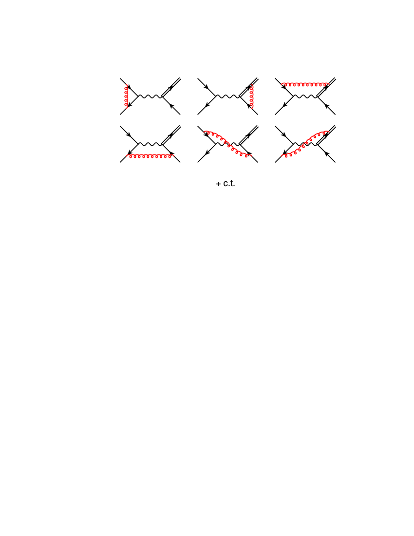
Figure 2: 1-loop Feynman diagrams for the hard function. The double line represents the top quark.

The hard function is a $2\times 2$ matrix in the color space. The RG equation it obeys reads

$$\frac{d\,\mathbf{H}}{d\ln\mu}=\mathbf{\Gamma}_{H}\mathbf{H}+\mathbf{H}\mathbf{\Gamma}^{\dagger}_{H}.$$ (39)

The relevant anomalous dimension matrix is process dependent and can be expanded in $\frac{\alpha_{s}}{4\pi}$, with the relevant expansion coefficient given in the appendix. The explicit form of the anomalous dimension matrix for s-channel single top production can be extracted from a more general result given in the Ref. [59]. Explicitly, for the independent color basis we have chosen, it is given by

$$\mathbf{\Gamma}_{H}=\left[\frac{3}{2}C_{F}\gamma_{\rm cusp}(\alpha_{s})\ln\frac{m^{2}_{t}}{\mu^{2}}+\bar{\gamma}_{h}(\alpha_{s})\right]\mathbf{1}+\mathbf{\Gamma}_{h},$$ (40)

with

$$\bar{\gamma}_{h}(\alpha_{s})=C_{F}\gamma_{\rm cusp}(\alpha_{s})\ln\frac{\hat{s}(\hat{s}-m^{2}_{t})}{m^{4}_{t}}+\gamma_{h}(\alpha_{s}),$$ (41)

and

$$\mathbf{\Gamma}_{h}=\gamma_{\rm cusp}(\alpha_{s})\left(\begin{array}[]{cc}0&\frac{C_{F}}{2N_{c}}\ln\frac{\hat{u}(\hat{u}-m^{2}_{t})}{\hat{t}(\hat{t}-m^{2}_{t})}\\ \ln\frac{\hat{u}(\hat{u}-m^{2}_{t})}{\hat{t}(\hat{t}-m^{2}_{t})}&\frac{N_{c}}{2}\ln\frac{\hat{u}(\hat{u}-m^{2}_{t})}{\hat{s}(\hat{s}-m^{2}_{t})}-\frac{1}{N_{c}}\ln\frac{\hat{u}(\hat{u}-m^{2}_{t})}{\hat{t}(\hat{t}-m^{2}_{t})}\end{array}\right).$$ (42)

The expression for $\gamma_{h}$ and $\gamma_{\rm cusp}$ can be found in the appendix. Note that we have only retained the real part of the anomalous dimension matrix. We have checked that the 1-loop hard function exactly obeys this equation, as it must. Details of it are presented in the appendix.

The solution of the RG equation shown in Eq. (39) can be obtained by diagonalizing the anomalous dimension matrix $\mathbf{\Gamma}_{h}$ [60]. A detail example for how to do this in effective field theory can be found in the Ref. [51]. To NNLL accuracy, the result can be expressed as

$$\mathbf{H}_{R}(\mu) = \exp[6S_{\rm DL}(\mu_{h},\mu)-2\bar{a}_{h}(\mu_{h},\mu)]\left(\frac{m^{3}_{t}}{\mu^{3}_{h}}\right)^{-2a_{\Gamma}(\mu_{h},\mu)}$$ (43)

$$\times\mathbf{U}_{R}(\mu_{h},\mu)\mathbf{H}(\mu_{h})\mathbf{U}^{\dagger}_{R}(\mu_{h},\mu),$$

with

$$\mathbf{U}_{R}(\mu_{h},\mu)=(\mathbf{1}+\frac{\alpha_{s}(\mu)}{4\pi}\mathbf{J})\left(\frac{\alpha_{s}(\mu_{h})}{\alpha_{s}(\mu)}\right)^{\mathbf{\Gamma}^{0}_{h}/(2\beta_{0})}(\mathbf{1}-\frac{\alpha_{s}(\mu_{h})}{4\pi}\mathbf{J}),$$ (44)

where

$$\mathbf{J}=\frac{\beta_{1}}{2\beta^{2}_{0}}\mathbf{\Gamma}^{0}_{h}-\frac{1}{2\beta_{0}}\mathbf{\Gamma}^{1}_{h}.$$ (45)

The Sudakov exponent are given by [34]:

$$S_{\rm DL}(\nu,\mu) = -\int^{\alpha_{s}(\mu)}_{\alpha_{s}(\nu)}\,d\lambda\frac{C_{F}\gamma_{\rm cusp}(\lambda)}{\beta(\lambda)}\int^{\lambda}_{\alpha_{s}(\nu)}\,\frac{d\lambda^{\prime}}{\beta(\lambda^{\prime})},$$

$$a_{\Gamma}(\nu,\mu) = -\int^{\alpha_{s}(\mu)}_{\alpha_{s}(\nu)}\,d\lambda\frac{C_{F}\gamma_{\rm cusp}(\lambda)}{\beta(\lambda)},$$

$$\bar{a}_{h}(\nu,\mu) = -\int^{\alpha_{s}(\mu)}_{\alpha_{s}(\nu)}\,d\lambda\frac{\bar{\gamma}_{h}(\lambda)}{\beta(\lambda)}.$$ (46)

Next, we discuss the jet function. Unlike the hard function which obeys a local RG equation, the jet function $J(p^{2},\mu)$ satisfies a RG equation which is non-local in $p^{2}$ [61]:

$$\frac{dJ(p^{2},\mu)}{d\ln\mu} = \left(-2C_{F}\gamma_{\rm cusp}(\alpha_{s})\ln\frac{p^{2}}{\mu^{2}}-2\gamma_{j}(\alpha_{s})\right)J(p^{2},\mu)$$ (47)

$$+2C_{F}\gamma_{\rm cusp}(\alpha_{s})\int^{p^{2}}_{0}dq^{2}\,\frac{J(p^{2},\mu)-J(q^{2},\mu)}{p^{2}-q^{2}}.$$

This equation is solved with the help of Laplace transformed jet function [61]:

$$\widetilde{j}(\ln\frac{Q^{2}}{\mu^{2}},\mu)=\int^{\infty}_{0}dp^{2}\,\exp(-\frac{p^{2}}{Q^{2}e^{\gamma_{E}}})J(p^{2},\mu),$$ (48)

which satisfies the RG equation

$$\frac{d\,\widetilde{j}(\ln\frac{Q^{2}}{\mu^{2}},\mu)}{d\ln\mu}=\left(-2C_{F}\gamma_{\rm cusp}(\alpha_{s})\ln\frac{Q^{2}}{\mu^{2}}-2\gamma_{j}(\alpha_{s})\right)\tilde{j}(\ln\frac{Q^{2}}{\mu^{2}},\mu),$$ (49)

and can be easily solved now. The solution, after transformed back to momentum space, is [61]

$${J}(p^{2},\mu)=\exp\left(-4S_{\rm DL}(\mu_{j},\mu)+2a_{j}(\mu_{j},\mu)\right)\widetilde{j}(\partial_{\eta_{j}},\mu_{j})\frac{1}{p^{2}}\left(\frac{p^{2}}{\mu^{2}_{j}}\right)^{\eta_{j}}\frac{e^{-\gamma_{E}\eta_{j}}}{\Gamma(\eta_{j})},$$ (50)

where $\eta_{j}=2a_{\Gamma}(\mu_{j},\mu)$.

Finally, we need the RG equation of the soft function, which can be obtained by noticing the fact that the hadronic cross section in the threshold region should be independent of the arbitrary scale $\mu$. Schematically,

$$\frac{d}{\ln\mu}f\otimes f\otimes\textbf{H}\otimes\textbf{S}\otimes J=0.$$ (51)

Based on this fact, we have

$$\widetilde{\mathbf{s}}\left(\ln\frac{\kappa}{\mu},\mu\right) = \int^{\infty}_{0}dk^{+}\exp\left(-\frac{k^{+}}{\kappa e^{\gamma_{E}}}\right)\mathbf{S}(k^{+},\mu),$$ (52)

$$\frac{d\,\widetilde{\mathbf{s}}\left(\ln\frac{\kappa}{\mu},\mu\right)}{d\ln\mu} = -\mathbf{\Gamma}^{\dagger}_{S}\widetilde{\mathbf{s}}\left(\ln\frac{\kappa}{\mu},\mu\right)-\widetilde{\mathbf{s}}\left(\ln\frac{\kappa}{\mu},\mu\right)\mathbf{\Gamma}_{S},$$ (53)

with

$$\mathbf{\Gamma}_{S} = \left(C_{F}\gamma_{\rm cusp}(\alpha_{s})\ln\frac{\kappa}{\mu}-\bar{\gamma}_{s}(\alpha_{s})\right)\mathbf{1}+\mathbf{\Gamma}_{h},$$ (54)

where

$$\bar{\gamma}_{s}(\alpha_{s})=-C_{F}\gamma_{\rm cusp}(\alpha_{s})\ln\frac{2n_{a}\!\cdot\!n_{b}\,v\!\cdot\!n_{1}}{n_{a}\!\cdot\!n_{1}\,n_{b}\!\cdot\!n_{1}}+\gamma_{s}(\alpha_{s}),$$ (55)

and $\gamma_{s}$ is given in the appendix. Note that in obtaining the RG equation Eq. (53), we have used the DGLAP evolution for the PDFs in the $x\to 1$ limit:

$$\frac{df_{q/N}(x,\mu)}{d\ln\mu}=2\gamma_{\phi}(\alpha_{s})f_{q/N}(x,\mu)+2C_{F}\gamma_{\rm cusp}(\alpha_{s})\int^{1}_{x}\frac{dz}{z}\frac{f_{q/N}(x/z,\mu)}{[1-z]_{+}}.$$ (56)

We stress that Eq. (53) is derived entirely from RG invariance of the resummed cross section in the threshold limit. If the explicit 1-loop soft function do obey this equation, it serves as a non-trivial check on the RG invariance of our result. We show in the appendix that this is indeed the case, as expected. The solution of the RG equation in momentum space is

$$\mathbf{S}_{R}(k^{+},\mu) = \exp[-2S_{\rm DL}(\mu_{s},\mu)-2\bar{a}_{s}(\mu_{s},\mu)]$$ (57)

$$\times\mathbf{U}^{\dagger}_{R}(\mu,\mu_{s})\widetilde{\mathbf{s}}(\partial_{\eta_{s}},\mu_{s})\mathbf{U}_{R}(\mu,\mu_{s})\frac{1}{k^{+}}\left(\frac{k^{+}}{\mu_{s}}\right)^{\eta_{s}}\frac{e^{-\gamma_{E}\eta_{s}}}{\Gamma(\eta_{s})},$$

where $\eta_{s}=2a_{\Gamma}(\mu_{s},\mu)$. Combining the above ingredients, we obtain the resummed cross section for s-channel single top production

$$\sigma^{\rm thres} = \sum_{ij}\frac{\pi}{4N^{2}_{c}E^{2}_{\rm CM}}\int^{1}_{0}\frac{dx_{a}}{x_{a}}\frac{dx_{b}}{x_{b}}\int\frac{d^{3}q}{2E_{q}(2\pi)^{3}}f_{i/N_{a}}(x_{a})f_{j/N_{b}}(x_{b})\lambda_{0,ij}$$ (58)

$$\times\int^{s_{4}/(2E_{1})}_{0}dk^{+}\,\mathrm{Tr}[\mathbf{H}_{R}(\mu)\mathbf{S}_{R}(k^{+},\mu)]J(s_{4}-2E_{1}k^{+},\mu),$$

where we have included a summation over different partonic channels.

5 NNLO expansion of resummed cross section

In the traditional approach to threshold resummation, the evolution equations for the factorized cross section are solved in Mellin moment space rather than momentum space. It has been demonstrated that in Drell-Yan production, the two approach are equivalent up to $1/N$ corrections when making the scale choices $\mu_{h}=M$ and $\mu_{s}=M/N$ [34]. Here $N$ is the Mellin moment and $M$ is the mass of the Drell-Yan lepton pair. Note that when $N$ is very large, the running coupling constant $\alpha_{s}(\mu_{s})$ blows up. Furthermore, in order to obtain the physical cross section in momentum space, one needs to invert the Mellin transformation numerically, which is ambiguous since the expression to be inverted has a Landau-pole for large $N$, although there have been several prescriptions for dealing with the Mellin inversion [62, 63, 64]. On the other hand, in the momentum space approach, we do not encounter such problem because $\mu_{s}$ is constrained to be well above the Landau-pole singularity.

It has also been advocated that the resummed cross section in Mellin moment space can be used as a generator of the fixed order perturbation expansion [65]. The ambiguity due to different Mellin inversion prescriptions can be avoided because at the fixed order no prescription is needed to invert the Mellin space results. In this way, partial NNNLO threshold singular terms were obtained for s-channel single top production [66, 67, 22].

In order to obtain the fixed order expansion in momentum space resummation formalism, we rewrite the cross section in terms of integral over singular distributions of $s_{4}$. In the center-of-mass frame of the top quark and the recoiling jet, we can parametrize the momentum of $\tilde{p}_{a}$, $\tilde{p}_{b}$ and $q$ as [68]

$$\tilde{p}_{a}=\frac{\sqrt{\hat{s}}}{2}(1,0,0,1),\quad\tilde{p}_{b}=\frac{\sqrt{\hat{s}}}{2}(1,0,0,-1),\quad q=(E_{q},0,|\mathbf{q}|\sin\chi,|\mathbf{q}|\cos\chi),$$ (59)

where

$$E_{q}=-\frac{\hat{t}+\hat{u}-2m^{2}_{t}}{2\sqrt{\hat{s}}},\quad\cos\chi=\frac{\hat{u}-\hat{t}}{\sqrt{(\hat{t}+\hat{u}-2m^{2}_{t})^{2}-4\hat{s}m^{2}_{t}}}.$$ (60)

Hence the phase space measure of the top quark is

$$\frac{d^{3}q}{2E_{q}(2\pi)^{3}} = \frac{1}{8\pi^{2}}dE_{q}d\chi\,\sin\chi\sqrt{E^{2}_{q}-m^{2}_{t}}$$ (61)

$$= \frac{1}{16\pi^{2}\hat{s}}d\hat{t}d\hat{u},$$

and the cross section can now be rewritten as

$$\sigma = \int^{1}_{m^{2}_{t}/s}d\tau\int^{1}_{\tau}\frac{dx_{a}}{x_{a}}\int^{0}_{m^{2}_{t}-\hat{s}}d\hat{t}\int^{s^{\rm max}_{4}}_{0}ds_{4}\,f_{i/N_{a}}(x_{a},\mu_{F})f_{j/N_{b}}(\tau/x_{a},\mu_{F})\frac{d\hat{\sigma}^{\rm thres}}{d\hat{t}d\hat{u}},$$ (62)

where $s^{\rm max}_{4}=\hat{s}+\hat{t}+m^{2}_{t}\hat{s}/(\hat{t}-m^{2}_{t})$, and

$$\frac{d\hat{\sigma}^{\rm thres}}{d\hat{t}d\hat{u}} = \sum_{ij}\frac{\lambda_{0,ij}}{64\pi N^{2}_{c}\hat{s}^{2}}\int^{s_{4}/(2E_{1})}_{0}dk^{+}\,\mathrm{Tr}[\mathbf{H}_{R}(\mu)\mathbf{S}_{R}(k^{+},\mu)]J(s_{4}-2E_{1}k^{+},\mu).$$ (63)

Following [34], we derive the threshold singular distributions by setting $\mu_{h}$, $\mu_{s}$ and $\mu_{j}$ equal to the common scale $\mu$, which is conveniently chosen as the factorization scale $\mu_{F}$. In the following, we show all the threshold singular distributions up to NNLO,

$$\frac{64\pi\hat{s}^{2}d^{2}\hat{\sigma}^{\rm expand}_{ij}}{\lambda_{0,ij}d\hat{t}\,d\hat{u}}=\delta(s_{4})+\frac{\alpha_{s}}{4\pi}\left(A_{2}D_{2}+A_{1}D_{1}+A_{0}\delta(s_{4})\right)$$

$$+\left(\frac{\alpha_{s}}{4\pi}\right)^{2}\left(B_{4}D_{4}+B_{3}D_{3}+B_{2}D_{2}+B_{1}D_{1}+B_{0}\delta(s_{4})\right),$$ (64)

where

$$D_{n}=\left[\frac{1}{s_{4}}\ln^{n-1}\frac{s_{4}}{m^{2}_{t}}\right]_{+}$$ (65)

is the conventional plus distribution, and its integral with a regular function $f(s_{4})$ is defined as

$$\int^{m^{2}_{t}}_{0}ds_{4}\,f(s_{4})D_{n}=\int^{m^{2}_{t}}_{0}ds_{4}\,[f(s_{4})-f(0)]\frac{1}{s_{4}}\ln^{n-1}\frac{s_{4}}{m^{2}_{t}}.$$ (66)

The coefficients $A_{n}$ and $B_{n}$ are given by

$$A_{2} = 3C_{F}\gamma^{0}_{\rm cusp},$$ (67)

$$A_{1} = C_{F}\gamma^{0}_{\rm cusp}(L_{h}+2L_{s})+\gamma^{0}_{j}-2\bar{\gamma}^{0}_{s},$$ (68)

$$A_{0} = \frac{c^{s}_{11}}{C^{2}_{A}}+c^{h}_{11}+c^{j}_{1}+C_{F}\gamma^{0}_{\rm cusp}\left(-\frac{L^{2}_{h}}{4}+L^{2}_{s}-\frac{\pi^{2}}{4}\right)+L_{h}(\gamma^{0}_{j}-\bar{\gamma}^{0}_{h})-2\bar{\gamma}^{0}_{s}L_{s},$$ (69)

$$B_{4} = \frac{9}{2}C^{2}_{F}(\gamma^{0}_{\rm cusp})^{2},$$ (70)

$$B_{3} = \frac{1}{2}C_{F}\gamma^{0}_{\rm cusp}\left(9C_{F}\gamma^{0}_{\rm cusp}L_{h}+18C_{F}\gamma^{0}_{\rm cusp}L_{s}+9\gamma^{0}_{j}-18\bar{\gamma}^{0}_{s}-5\beta_{0}\right),$$ (71)

$$B_{2} = C_{F}\gamma^{0}_{\rm cusp}\left[\frac{3c^{s}_{11}}{C^{2}_{A}}+3c^{h}_{11}+3c^{j}_{1}-L_{h}(3\bar{\gamma}^{0}_{h}-5\gamma^{0}_{j}+4\bar{\gamma}^{0}_{s}+\beta_{0})+4\gamma^{0}_{j}L_{s}-14\bar{\gamma}^{0}_{s}L_{s}\right.$$ (73)

$$\left.-4L_{s}\beta_{0}\right]+\frac{C_{F}((\Gamma^{0}_{h,21})^{2}+3C_{A}\gamma^{1}_{\rm cusp})}{C_{A}}+2\Gamma^{0}_{h,12}\Gamma^{0}_{h,21}+\frac{1}{4}C^{2}_{F}(\gamma^{0}_{\rm cusp})^{2}$$

$$\times[(L_{h}+2L_{s})(L_{h}+14L_{s})-9\pi^{2}]-\beta_{0}(\gamma^{0}_{j}-4\bar{\gamma}^{0}_{s})-4\gamma^{0}_{j}\bar{\gamma}^{0}_{s}+(\gamma^{0}_{j})^{2}+4(\bar{\gamma}^{0}_{s})^{2},$$

$$B_{1} = \frac{1}{12C^{2}_{A}}C_{F}\gamma^{0}_{\rm cusp}\left[3C^{2}_{A}[4L_{h}(c^{h}_{11}-2L_{s}(\bar{\gamma}^{0}_{h}-\gamma^{0}_{j}+\bar{\gamma}^{0}_{s}))+8L_{s}c^{h}_{11}+4c^{j}_{1}(L_{h}+2L_{s})\right.$$ (74)

$$+L^{2}_{h}(-4\bar{\gamma}^{0}_{h}+3\gamma^{0}_{j}+2\bar{\gamma}^{0}_{s})+4\gamma^{0}_{j}L^{2}_{s}-3\pi^{2}\gamma^{0}_{j}-24\bar{\gamma}^{0}_{s}L^{2}_{s}+6\pi^{2}\bar{\gamma}^{0}_{s})]$$

$$\left.+12c^{s}_{11}(L_{h}+2L_{s})+C^{2}_{A}\beta_{0}(5\pi^{2}-6(L^{2}_{h}+4L^{2}_{s}))\right]$$

$$+C_{F}\left[\frac{\Gamma^{0}_{h,21}}{2C_{A}}(2c^{h}_{12}-\Gamma^{0}_{h,21}(L_{h}+2L_{s}))+\gamma^{1}_{\rm cusp}(L_{h}+2L_{s})\right]$$

$$+\frac{1}{C^{2}_{A}}(2\Gamma^{0}_{h,21}c^{s}_{12}+c^{s}_{11}(\gamma^{0}_{j}-2(\bar{\gamma}^{0}_{s}+\beta_{0})))+2\Gamma^{0}_{h,12}c^{h}_{12}+(2L_{s}-L_{h})\Gamma^{0}_{h,12}\Gamma^{0}_{h,21}$$

$$+c^{h}_{11}(\gamma^{0}_{j}-2\bar{\gamma}^{0}_{s})-\frac{C^{2}_{F}}{4}(\gamma^{0}_{\rm cusp})^{2}[(L_{h}+2L_{s})(L^{2}_{h}-4L^{2}_{s}+3\pi^{2})-36\zeta_{3}]$$

$$+c^{j}_{1}(\gamma^{0}_{j}-2\bar{\gamma}^{0}_{s}-\beta_{0})-\bar{\gamma}^{0}_{h}\gamma^{0}_{j}L_{h}+2\bar{\gamma}^{0}_{h}\bar{\gamma}^{0}_{s}L_{h}-2\gamma^{0}_{j}\bar{\gamma}^{0}_{s}L_{h}-2\gamma^{0}_{j}\bar{\gamma}^{0}_{s}L_{s}-\gamma^{0}_{j}\beta_{0}L_{h}$$

$$+(\gamma^{0}_{j})^{2}L_{h}+\gamma^{1}_{j}+4\bar{\gamma}^{0}_{s}\beta_{0}L_{s}+4(\bar{\gamma}^{0}_{s})^{2}L_{s}-2\bar{\gamma}^{1}_{s},$$

where $L_{h}=\ln\frac{m^{2}_{t}}{\mu^{2}}$ and $L_{s}=\ln\frac{m^{2}_{t}\sqrt{\hat{s}}}{(\hat{s}-m^{2}_{t})\mu}$. Explicit expressions for $c^{h}$, $c^{s}$ and $c^{j}$ are given in the appendix. Several comments on this result are in order. Our NNLO expansion are accurate to NNLL accuracy, i.e., the coefficients $A_{2,1,0}$ and $B_{4,3,2,1}$ are accurate. Complete expression for $B_{0}$ can only be known from a 2-loop calculation, therefore we retain from giving a partial result for it here. Similar expansion has been performed in the Ref. [22], but only partial NNLL logarithms are presented. In particular, the coefficient of $D_{2}$ and $D_{1}$ at NNLO is not complete in [22], because of the omission of virtual corrections in their work. We also note that due to different definition of $s_{4}$, in order to comparison with the result in the Ref. [22], we have to make the follwing change to $\bar{\gamma}_{s}$

$$\bar{\gamma}_{s}=-C_{F}\gamma_{\rm cusp}\ln\frac{(\hat{s}-m^{2}_{t})^{2}\sqrt{\hat{s}}}{\hat{u}\hat{t}m_{t}}+\gamma_{s}\rightarrow-C_{F}\gamma_{\rm cusp}\ln\frac{(\hat{s}-m^{2}_{t})^{2}\sqrt{\hat{s}}}{(\hat{u}-m^{2}_{t})(\hat{t}-m^{2}_{t})m_{t}}+\gamma_{s}.$$ (75)

We have checked that our expression for $B_{4,3}$ agree with the Ref. [22] after this replacement. We also checked that our $\mu$ dependence in the expansion coefficients agree with [22] for $A_{2,1}$ and $B_{4,3,2}$ after this replacement. There is an extra $\mu$ dependence term in $B_{4}$ of our expansion, $C_{F}\gamma^{0}_{\rm cusp}L_{h}c^{h}_{11}$, which is not presented in [22]. There is also $\mu$ dependence in $B_{0}$. However we are not able to check this term against [22] since the explicit expression for this term is not presented there. We give a numerical comparison on the difference of different threshold variable definition and the effects of omitting virtual corrections in the resummation result in next section.

6 Numerical discussion

In this section, we present the numerical results for the threshold resummation effects on the s-channel single top production at both the Tevatron and the LHC. The input parameters used throughout this section are given below:

$$\begin{gathered}m_{t}=173.2\;{\rm{GeV}},\quad M_{W}=80.4\;{\rm{GeV}},\quad G_{F}=1.16639\times 10^{-5}\;{\rm{GeV}},\\ V_{\rm CKM}=\left(\begin{tabular}[]{ccc}0.9751&0.2210&0\\ 0.2215&0.9743&0\\ 0.0035&0.0410&1\end{tabular}\right).\end{gathered}$$

We use the MSTW2008NNLO PDFs [69] throughout our numerical calculation.

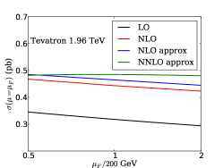
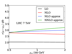
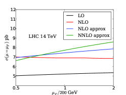
Figure 3: Factorization scale dependence of NNLO expanded cross sections for s-channel single top production at the Tevatron ($1.96$ TeV) and LHC ($7$ TeV and $14$ TeV).

Before presenting the numerical results for resummed cross section, it’s important to examine to what extent the singular terms approximate the fixed order calculation. It would be meaningless if the neglected subleading terms are as important as the singular terms. We present the numerical results for the approximate NLO and NNLO cross section, Eq. (64), for both Tevatron and LHC in Fig. 3. The factorization scale is chosen as $\mu_{F}=200$ GeV, as will be explained below. It can be seen from Fig. 3 that at the Tevatron, which has a lower collision energy, the approximate NLO cross section over estimates the exact NLO cross section by about $5\%$. Since the NLO corrections for s-channel single top production is quite large, about $40\%$ at the Tevatron, we consider the threshold expansion as a good approximation. Furthermore, the fact that the scale dependence of the approximate NLO result is similar to exact NLO result implies the small scale dependence of the subleading terms. On the other hand, the NLO approximation doesn’t work well at the LHC with higher collision energy at $7$ TeV or $14$ TeV, as shown in Fig. 3. The differences mentioned above are smaller at lower factorization scale and more significant at larger factorization scale. Moreover, the scale dependence of the approximate NLO cross section behave quite differently from the exact NLO results, indicating that the subleading terms are not only numerically large, but also have large impact on the factorization scale dependence of the cross section. Therefore, we conclude that our resummation results at the LHC are not as reliable as at the Tevatron. Nevertheless, we still give the NNLO approximate and resummed results for both the Tevatron and the LHC as a reference.

In order to calculate the resummed cross section, Eq. (58), we need to determine the appropriate scales for the process. In the SCET approach to resummation, there are four scales: the hard scale $\mu_{h}$, the jet scale $\mu_{j}$, the soft scale $\mu_{s}$, and the factorization scale $\mu_{F}$, and we have assumed that the renormalization scale equals the factorization scale for simplicity. This is different from the fixed order calculation, where only the factorization scale is accessible. This is actually the merit of effective theory, since the calculation has been factorized into a series of single-scale problems, and large logarithms can be avoided if appropriate value of scale is chosen for each problem.

First, we choose a default value for the hard scale. Since s-channel single top production is similar to the Drell-Yan process, one would expect that the appropriate value of the hard scale should be around $\sqrt{\hat{s}}$. However, choosing $\mu_{h}\sim\sqrt{\hat{s}}$ is inconvenient because $\sqrt{\hat{s}}$ is a dynamical variable. To avoid this inconvenience we set the hard scale at a fixed value, $\mu_{h}=200$ GeV, which is slightly larger than $m_{t}$. We have checked that invariant mass distribution of the virtual $W$ boson peaks around this value, and thus it can be considered as the “average” value of $\sqrt{\hat{s}}$. For simplicity, we also choose the factorization scale to be $200$ GeV.

Next, we determine the appropriate soft scale and jet scale. In order to obtain a reasonable physical result, we expect that no large logarithms should arise in the soft and jet function when the appropriate scales are chosen. In practice, for the determination of soft scale (jet scale), we fix the factorization scale at $200$ GeV in the factorized cross section Eq. (58), and set all the other scales equal to $\mu_{s}$ ($\mu_{j}$), and then vary $\mu_{s}$ ($\mu_{j}$). In Fig. 4, we plot the cross section which only include the one-loop soft corrections or jet corrections, respectively, divided by the tree-level cross section with all scales equal to $200$ GeV. From Fig. 4, we find that the net corrections are small around $\mu_{j}=50$ GeV for the jet corrections. Thus we take it as our default scale choice for jet scale. The choice of soft scale is not as clear as jet scale from Fig. 4 since the total soft corrections do not have a clear minimum or maximum. The reason is that at NLO, the soft corrections consist of a Drell-Yan like corrections in the initial state and a soft gluon corrections in the final state, as depicted in graphs (a), (b) and (c) of Fig. 1. It turns out that the corrections is positive in the initial state and negative in the final state. Either initial state corrections or final state corrections show an appropriate scale around $25$ GeV, but not the sum. On the other hand, an appropriate choice for soft scale is dictated by the picture of underlying factorization, $\mu_{s}\sim\mu^{2}_{j}/\mu_{h}$. From our choice for hard and jet scale, this implies that soft scale should be chosen around $10-30$ GeV. In our numerical calculation, we have chosen $\mu_{s}$ as $25$ GeV, to avoid too close to $\Lambda_{\rm QCD}$ while probe as much soft activity as possible.

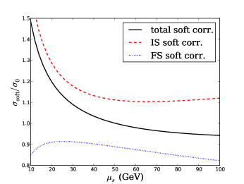
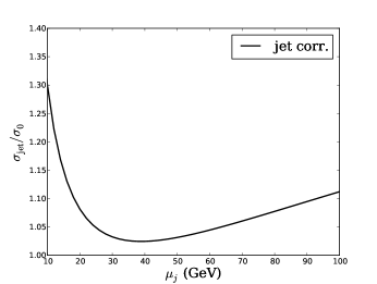
Figure 4: Determination of $\mu_{s}$ and $\mu_{j}$. On the left (right) is the cross section with only soft (jet) corrections, divided by the tree-level cross section, for the variation of $\mu_{s}$ ($\mu_{j}$). The red dashed line includes only the initial state soft corrections, while the blue dotted line includes only the final state soft corrections. The factorization scale is fixed at $200$ GeV.

We also note that the factorized cross section Eq. (58) is derived in the threshold limit, $s_{4}\to 0$. To capture the non-leading terms, we must match the resummed cross section onto the NLO cross section, which can be found in the Ref. [3]. We have redone the calculation and found complete agreement with the Ref. [3]. After matching in momentum space approach, the resummed total cross sections is given by

$$\sigma^{\rm RES}=\sigma^{\rm thres}-\left.\sigma^{\rm thres}\right|_{\mu_{h}=\mu_{j}=\mu_{s}=\mu_{F}}+\left.\sigma^{\rm NLO}\right|_{\mu_{F}}.$$ (76)

In table 1, we present the resummed total cross section for s-channel single top and anti-top production, as well as the NNLO approximation at both the Tevatron and the LHC. All the scales are set to the default values, i.e., $\mu_{F}=\mu_{h}=200$ GeV, $\mu_{s}=25$ GeV and $\mu_{j}=50$ GeV. It can be seen that the NLO QCD corrections significantly enhance the total cross section at both the Tevatron and the LHC [3]. The threshold resummation effects further increase the NLO cross section by about $3\%-5\%$ at the Tevatron. However, we do not observe the large enhancement due to threshold resummation as reported in Ref. [22]. The discrepancy has two origin. First, the 1-loop matching coefficients of hard function was not taken into account in [22]. second, the definiton of $s_{4}$ used in [22] does not coincide with ours. As explained in Sec. 3, the definition we use also include the effects of collinear splitting of final state b-quark, and should be considered as a better choice. We quantify the numerical significance of the difference from these different treatment in the end of this section briefly. We also show the resummed cross section for single top production at the Tevatron for different top quark mass in Fig. 5. It can be seen that the LO prediction significantly under estimates the total cross section. It’s also clear that the resummed cross section dramatically improves the scale dependence, comparing with the NLO results.

	$\sigma_{\rm LO}$	$\sigma_{\rm NLO}$	$\sigma_{\rm expand}$	$\sigma_{\rm RES}$
Tevatron (top)	$0.318^{+0.029}_{-0.024}$ pb	$0.443^{+0.024}_{-0.020}$ pb	$0.463^{+0.002}_{-0.004}$ pb	$0.467^{+0.010}_{-0.010}$ pb
Tevatron (anti-top)	$0.318^{+0.029}_{-0.024}$ pb	$0.443^{+0.024}_{-0.020}$ pb	$0.463^{+0.002}_{-0.004}$ pb	$0.467^{+0.010}_{-0.010}$ pb
LHC ($7$ TeV, top)	$2.03^{+0.01}_{-0.01}$ pb	$2.71^{+0.07}_{-0.05}$ pb	$2.82^{+0.06}_{-0.07}$ pb	$2.81^{+0.16}_{-0.10}$ pb
LHC ($7$ TeV, anti-top)	$1.14^{+0.01}_{-0.01}$ pb	$1.53^{+0.04}_{-0.03}$ pb	$1.60^{+0.03}_{-0.04}$ pb	$1.60^{+0.08}_{-0.05}$ pb
LHC ($14$ TeV, top)	$5.21^{+0.14}_{-0.18}$ pb	$6.91^{+0.09}_{-0.05}$ pb	$7.17^{+0.20}_{-0.25}$ pb	$7.11^{+0.47}_{-0.35}$ pb
LHC ($14$ TeV, anti-top)	$3.36^{+0.09}_{-0.12}$ pb	$4.46^{+0.03}_{-0.05}$ pb	$4.64^{+0.10}_{-0.18}$ pb	$4.61^{+0.28}_{-0.24}$ pb

Table 1: Total cross section for single top and anti-top production at the Tevatron and LHC. All the scales are chosen at the default values. For the resummed results, The total uncertainties are obtained by adding the individual scale variations of $\mu_{F},\mu_{h},\mu_{j},\mu_{s}$ in quadrature.

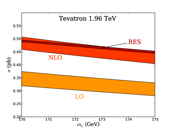
Figure 5: Top quark mass dependence of the fixed order and resummed cross section. The band corresponds to the variation of factorization scale around $200$ GeV by a factor of 2.

Finally, we give a brief numerical comparision with results presented in Ref. [22]. As mentioned in the last section, our NNLO singular expansion differ from those presented in [22] in two aspects: (a) We have included all the 1-loop matching coeffcients $c^{h},c^{s},c^{j}$ in our calculation. Therefore our results contain all the NNLL logarithms.  (b) The results in the Ref. [22] used a different definition of $s_{4}$, as was mentioned in Sec. 3. To quantify the effects of these differences, we plot two sets of cross sections below. In Fig. 6, we plot the NNLO approximate result with $c^{h}_{ij}$ set to zero. As can be seen from the figure, the NLO or NNLO approximation fail to approximate the exact NLO result when the virtual corrections are off, which give large positive contribution at the NLO. In Fig. 7, we plot the NNLO approximate results with the same definition of $s_{4}$ as in Ref. [22]. The NLO or NNLO approximate cross sections are significantly enhanced with such choice for $s_{4}$, and overestimate the exact NLO results by a large amount.

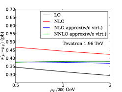
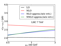
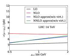
Figure 6: Illustration of the importance of the NLO virtual corrections in the NNLO expansion. We have set $c^{h}_{ij}$ to zero in these plots.

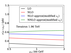
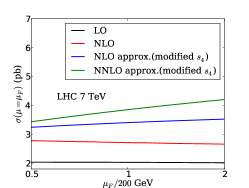
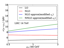
Figure 7: Illustration of the effects of different threshold variable definition. We have chosen the same $s_{4}$ definition as Ref. [22] in these plots.

7 Conclusions

We have studied the production of s-channel single top quark in the SM at both the Tevatron and the LHC. Using SCET, we show that the production cross section can be factorized into a convolution of hard function, soft function and jet function in the threshold limit. Each function, being sensitive to a single scale, is free of large logarithms once an appropriate scale is chosen. By this way, the threshold resummation is performed with the conventional RG equation. As a by-product, we obtain a NNLO expansion of threshold singular distributions. We also perform a numerical investigation of our resummed formula, using the momentum space resummation formalism [30]. We find that in general, the higher order threshold logarithms enhance the NLO cross sections by about $3\%-5\%$ at the Tevatron, and the resummation effects significantly reduce the factorization scale dependence of the total cross section at the Tevatron, while at the LHC the factorization scale dependence has not been improved, compared with the NLO results.

Appendix A Relevant anomalous dimensions and matching coefficients

The various anomalous dimensions needed in our resummation can be found, e.g., in the Refs [61, 34, 47]. We list them below for the convenience of the reader. The QCD $\beta$ function is

$$\beta(\alpha_{s})=-2\alpha_{s}\left[\beta_{0}\frac{\alpha_{s}}{4\pi}+\beta_{1}\left(\frac{\alpha_{s}}{4\pi}\right)^{2}+\cdots\right],$$ (77)

with expansion coefficients

$$\beta_{0} = \frac{11}{3}C_{A}-\frac{4}{3}T_{F}n_{f},$$

$$\beta_{1} = \frac{34}{3}C^{2}_{A}-\frac{20}{3}C_{A}T_{F}n_{f}-4C_{F}T_{F}n_{f},$$

$$\beta_{2} = \frac{2857}{54}C^{3}_{A}+\left(2C^{2}_{F}-\frac{205}{9}C_{F}C_{A}-\frac{1415}{27}C^{2}_{A}\right)T_{F}n_{f}+\left(\frac{44}{9}C_{F}+\frac{158}{27}C_{A}\right)T^{2}_{F}n^{2}_{f},$$ (78)

where $C_{A}=3$, $T_{F}=1/2$ for QCD, and $n_{f}$ is the number of active quark flavor.

The cusp anomalous dimension is

$$\gamma_{\rm cusp}(\alpha_{s})=\gamma^{0}_{\rm cusp}\frac{\alpha_{s}}{4\pi}+\gamma^{1}_{\rm cusp}\left(\frac{\alpha_{s}}{4\pi}\right)^{2}+\cdots,$$ (79)

with

$$\gamma^{0}_{\rm cusp} = 4,$$

$$\gamma^{1}_{\rm cusp} = 4\left[\left(\frac{67}{9}-\frac{\pi^{2}}{3}\right)C_{A}-\frac{20}{9}T_{F}n_{f}\right],$$

$$\gamma^{2}_{\rm cusp} = 4\left[C^{2}_{A}\left(\frac{245}{6}-\frac{134}{27}\pi^{2}+\frac{11}{45}\pi^{4}+\frac{22}{3}\zeta_{3}\right)+C_{A}T_{F}n_{f}\left(-\frac{418}{27}+\frac{40}{27}\pi^{2}-\frac{56}{3}\zeta_{3}\right)\right.$$ (80)

$$\left.+C_{F}T_{F}n_{f}\left(-\frac{55}{3}+16\zeta_{3}\right)-\frac{16}{27}T^{2}_{F}n^{2}_{f}\right].$$

The other anomalous dimensions are expanded as Eq. (79), and their expansion coefficients are

$$\gamma^{0}_{q} = -3C_{F},$$

$$\gamma^{1}_{q} = C^{2}_{F}\left(-\frac{3}{2}+2\pi^{2}-24\zeta_{3}\right)+C_{F}C_{A}\left(-\frac{961}{54}-\frac{11}{6}\pi^{2}+26\zeta_{3}\right)+C_{F}T_{F}n_{f}\left(\frac{130}{27}+\frac{2}{3}\pi^{2}\right),$$

$$\gamma^{0}_{Q} = -2C_{F},$$

$$\gamma^{1}_{Q} = C_{F}C_{A}\left(\frac{2}{3}\pi^{2}-\frac{98}{9}-4\zeta_{3}\right)+\frac{40}{9}C_{F}T_{F}n_{f},$$

$$\gamma^{0}_{\phi} = 3C_{F},$$

$$\gamma^{1}_{\phi} = C^{2}_{F}\left(\frac{3}{2}-2\pi^{2}+24\zeta_{3}\right)+C_{F}C_{A}\left(\frac{17}{6}+\frac{22}{9}\pi^{2}-12\zeta_{3}\right)-C_{F}T_{F}n_{f}\left(\frac{2}{3}+\frac{8}{9}\pi^{2}\right),$$

$$\gamma^{0}_{j} = -3C_{F},$$

$$\gamma^{1}_{j} = C^{2}_{F}\left(-\frac{3}{2}+2\pi^{2}-24\zeta_{3}\right)+C_{F}C_{A}\left(-\frac{1769}{54}-\frac{11}{9}\pi^{2}+40\zeta_{3}\right)$$ (81)

$$+C_{F}T_{F}n_{f}\left(\frac{242}{27}+\frac{4}{9}\pi^{2}\right),$$

$\gamma_{h}$ and $\gamma_{s}$ can be obtained from the anomalous dimensions above through the following equations:

$$\gamma_{h} = 3\gamma_{q}+\gamma_{Q},$$

$$\gamma_{s} = -2\gamma_{\phi}-\gamma_{h}+\gamma_{j}.$$ (82)

The hard function is a $2\times 2$ matrix in color space. To $\mathcal{O}(\alpha_{s})$, it can be written as

$$\textbf{H}=\left(\begin{array}[]{cc}1+\frac{\alpha_{s}}{4\pi}H^{1}_{11}&\frac{\alpha_{s}}{4\pi}H^{1}_{12}\\ \frac{\alpha_{s}}{4\pi}H^{1}_{21}&0\end{array}\right).$$ (83)

$H^{1}_{11}$ can be obtained from evaluating the first two diagrams of Fig. 2 and the corresponding counter-terms. It is given by

$$H^{1}_{11}=-\frac{3}{4}C_{F}\gamma^{0}_{\rm cusp}(\alpha_{s})\ln^{2}\frac{m^{2}_{t}}{\mu^{2}}-\bar{\gamma}^{0}_{h}\ln\frac{m^{2}_{t}}{\mu^{2}}+c^{h}_{11},$$ (84)

with

$$c^{h}_{11} = C_{F}\left[2\frac{\hat{u}}{\hat{t}-m^{2}_{t}}x_{t}\ln\frac{x_{t}}{1-x_{t}}+\ln(1-x_{t})(-2x_{t}+8\ln x_{t}+6)-6\ln^{2}(1-x_{t})\right.$$ (85)

$$\left.-4{\rm Li}_{2}\left(\frac{x_{t}}{x_{t}-1}\right)-4\ln^{2}x_{t}+(2x_{t}-12)\ln x_{t}+\frac{29}{6}\pi^{2}-28\right],$$

where $x_{t}=m^{2}_{t}/\hat{s}$. We have checked this result against the existing NLO virtual corrections to s-channel single top production [3] and found complete agreement. The remaining diagrams of Fig. 2 corresponds to $H^{1}_{12}$ and $H^{1}_{21}$. They do not contribute to the cross section at the NLO but do at the NNLO, therefore are required for a complete NNLL resummation. The results are

$$H^{1}_{12}=H^{1}_{21}=\frac{1}{2}\gamma_{\rm cusp}^{0}\ln\frac{\mu^{2}}{m^{2}_{t}}\ln\frac{\hat{u}(\hat{u}-m^{2}_{t})}{\hat{t}(\hat{t}-m^{2}_{t})}+c^{h}_{12},$$ (86)

with

$$\frac{\hat{t}(\hat{t}-m^{2}_{t})}{\hat{s}-M^{2}_{W}}c^{h}_{12}$$ (87)

$$= -2\left[m^{2}_{t}(\hat{s}+2\hat{t})+M^{2}_{W}\hat{s}-\hat{s}^{2}-2\hat{s}\hat{t}-2\hat{t}^{2}\right]C_{0}(0,0,\hat{s},M^{2}_{W},0,0)$$

$$+\frac{1}{\hat{s}+\hat{t}}\left[m^{2}_{t}(\hat{t}(3\hat{t}-2M^{2}_{W})+\hat{s}^{2}+4\hat{s}\hat{t})+(\hat{s}+\hat{t})^{2}(M^{2}_{W}-\hat{s}-2\hat{t})\right]C_{0}(0,\hat{u},m^{2}_{t},M^{2}_{W},0,0)$$

$$+4\hat{t}(m^{2}_{t}-\hat{t})C_{0}(0,0,\hat{s},0,0,M^{2}_{W})-\hat{u}(M^{2}_{W}+\hat{u}-\hat{t})C_{0}(0,0,\hat{u},0,0,0)$$

$$+(m^{2}_{t}-\hat{s})(M^{2}_{W}+\hat{u}-\hat{t})C_{0}(0,\hat{s},m^{2}_{t},0,0,M^{2}_{W})-\hat{u}(M^{2}_{W}+\hat{u}-\hat{t})C_{0}(0,\hat{u},0,M^{2}_{W},0,m^{2}_{t})$$

$$+(\hat{s}+\hat{t})(M^{2}_{W}+\hat{u}-\hat{t})C_{0}(m^{2}_{t},0,\hat{u},m^{2}_{t},0,0)+2m^{2}_{t}\hat{t}C_{0}(0,\hat{t},0,M^{2}_{W},0,m^{2}_{t})$$

$$\frac{1}{m^{2}_{t}-\hat{s}}\left[m^{6}_{t}+m^{4}_{t}(M^{2}_{W}-3\hat{s}-2\hat{t})+m^{2}_{t}(3\hat{s}(\hat{s}+2\hat{t})-2M^{2}_{W}(\hat{s}+\hat{t}))+\hat{s}^{2}(M^{2}_{W}-\hat{s}-2\hat{t})\right]$$

$$\times C_{0}(m^{2}_{t},\hat{s},0,m^{2}_{t},0,M^{2}_{W})-2\hat{t}^{2}(m^{2}_{t}-\hat{t})D_{0}(0,0,0,m^{2}_{t},\hat{t},\hat{s},0,0,0,M^{2}_{W})$$

$$2\hat{t}(m^{2}_{t}-\hat{t})^{2}D_{0}(0,\hat{s},0,\hat{t},m^{2}_{t},0,m^{2}_{t},M^{2}_{W},0,0)$$

$$+(\hat{s}+\hat{t})\left[m^{2}_{t}(M^{2}_{W}-\hat{s}-2\hat{t})+M^{4}_{W}-2M^{2}_{W}(\hat{s}+\hat{t})+\hat{s}^{2}+2\hat{s}\hat{t}+2\hat{t}^{2}\right]$$

$$\times D_{0}(m^{2}_{t},0,0,0,\hat{u},\hat{s},m^{2}_{t},0,0,M^{2}_{W})$$

$$-\Big{[}m^{4}_{t}(M^{2}_{W}-\hat{s}-2\hat{t})+m^{2}_{t}(M^{4}_{W}-3M^{2}_{W}(\hat{s}+\hat{t})+2\hat{s}^{2}+5\hat{s}\hat{t}+4\hat{t}^{2})$$

$$-M^{4}_{W}(\hat{s}+\hat{t})+2M^{2}_{W}(\hat{s}+\hat{t})^{2}-\hat{s}^{3}-3\hat{s}^{2}\hat{t}-4\hat{s}\hat{t}^{2}-2\hat{t}^{3}\Big{]}D_{0}(0,0,0,m^{2}_{t},\hat{s},\hat{u},M^{2}_{W},0,0,0)$$

$$+\frac{2m^{2}_{t}\hat{t}(\hat{u}-\hat{s})}{(m^{2}_{t}-\hat{s})(\hat{s}+\hat{t})}(B_{0}(m^{2}_{t},0,M^{2}_{W})+B_{0}(m^{2}_{t},0,m^{2}_{t}))+\frac{4\hat{s}\hat{t}}{m^{2}_{t}-\hat{s}}B_{0}(\hat{s},0,M^{2}_{W})$$

$$-\frac{2\hat{t}\hat{u}}{\hat{s}+\hat{t}}(B_{0}(\hat{u},0,0)+B_{0}(\hat{u},0,m^{2}_{t}))-\frac{2}{\epsilon_{\rm IR}}\frac{\hat{t}(\hat{t}-m^{2}_{t})}{\hat{s}-M^{2}_{W}}\ln\frac{\hat{u}(\hat{u}-m^{2}_{t})}{\hat{t}(\hat{t}-m^{2}_{t})},$$

where the $B_{0}$, $C_{0}$ and $D_{0}$ are the conventional Passarino-Veltman function [70], evaluated at the point where the ’t Hooft mass is set to $m_{t}$. For example, the $B_{0}$ function reads

$$B_{0}(p^{2}_{1},m^{2}_{1},m^{2}_{2})=\frac{m^{2\epsilon}_{t}\Gamma(1-\epsilon)}{i\pi^{2-\epsilon}}\int\,d^{4-2\epsilon}l\,\frac{1}{(l^{2}-m^{2}_{1}+i\varepsilon)((l+p_{1})^{2}-m^{2}_{2}+i\varepsilon)},$$ (88)

and similarly for $C_{0}$ and $D_{0}$. This is just a simple way to extract the $\mu$ dependece from $H^{1}_{12}$. The analytical form of the singular Passarino-Veltman function can be found, e.g., in the Ref. [71]. Note that $H^{1}_{12}$ and $H^{1}_{21}$ are UV and IR finite. Given the 1-loop matching coefficient above, one can check that the RG evolution equation of the hard function exactly has the form of Eq. (39).

The calculation of the soft function can be divided into the calculations of soft integral $I_{S}$ and the corresponding color factor. We first discuss the soft integral below. The soft integral corresponding to diagram (a) of Fig. 1 and its mirror image counterpart can be written as

$$I_{a}=2g^{2}_{s}\left(\frac{\mu^{2}e^{\gamma_{E}}}{4\pi}\right)^{\epsilon}\int\,\frac{d^{n}q}{(2\pi)^{n-1}}\delta(q^{2})\theta(q_{0})\delta(k^{+}-n_{1}\cdot q)\frac{n_{a}\cdot n_{b}}{(n_{a}\cdot q)(n_{b}\cdot q)},$$ (89)

where we work in $n=4-2\epsilon$ dimension, and the factor of 2 comes from doubling the contribution of diagram (a) by including its mirror image counterpart. This integral is evaluated by Becher and Schwartz [47], with the result:

$$\bar{I}_{a}=\frac{\alpha_{s}}{4\pi}\left\{\left[2\ln^{2}\frac{2n_{ab}}{n_{1a}n_{1b}}-\frac{\pi^{2}}{3}\right]\delta(k^{+})+16\left[\frac{1}{k^{+}}\ln\left(\frac{k^{+}}{\mu}\sqrt{\frac{2n_{a}\cdot n_{b}}{n^{+}_{a}n^{+}_{b}}}\right)\right]^{[k^{+},\mu]}_{\star}\right\},$$ (90)

where $n^{+}_{a(b)}=n_{a(b)}\cdot n_{1}$ and $[f]^{[a,b]}_{\star}$ is the star distribution defined in the Ref. [45]. Note that we have put a bar on $I$ to denote that divergent terms have been subtracted in $\overline{\text{MS}}$ scheme.

The soft integral corresponding to diagram (b) and (c) of Fig. 1 reads

$$I_{b} = -g^{2}_{s}\left(\frac{\mu^{2}e^{\gamma_{E}}}{4\pi}\right)^{\epsilon}\int\,\frac{d^{n}q}{(2\pi)^{n-1}}\delta(q^{2})\theta(q_{0})\delta(k^{+}-n_{1}\cdot q)\frac{1}{(v\cdot q)^{2}},$$ (91)

$$I_{c} = 2g^{2}_{s}\left(\frac{\mu^{2}e^{\gamma_{E}}}{4\pi}\right)^{\epsilon}\int\,\frac{d^{n}q}{(2\pi)^{n-1}}\delta(q^{2})\theta(q_{0})\delta(k^{+}-n_{1}\cdot q)\frac{v^{+}}{(n_{1}\cdot q)(v\cdot q)},$$ (92)

where $v^{+}=v\cdot n_{1}$. The simplest way to do the integral of $I_{b}$ and $I_{c}$ is working in the lightlike coordinates along the $n_{1}$ direction, in which any four vector can be written as

$$p^{\mu}=\frac{1}{2}p^{-}n^{\mu}_{1}+\frac{1}{2}p^{+}\bar{n}^{\mu}_{1}+p^{\mu}_{\perp}.$$ (93)

The results for the integrals in Eqs. (91) and (92) are

$$\bar{I}_{b} = \frac{\alpha_{s}}{4\pi}\left\{4\ln v^{+}\delta(k^{+})-4\left[\frac{1}{k^{+}}\right]^{[k^{+},\mu]}_{\star}\right\},$$ (94)

$$\bar{I}_{c} = \frac{\alpha_{s}}{4\pi}\left\{\left[-4\ln^{2}v^{+}-\frac{\pi^{2}}{6}\right]\delta(k^{+})-8\left[\frac{1}{k^{+}}\ln\frac{k^{+}}{v^{+}\mu}\right]^{[k^{+},\mu]}_{\star}\right\}.$$ (95)

The next two diagrams, (d) and (e), vanish, as was explained in the Ref. [47]. Diagrams (f) and (g) are the most complicated diagrams to be evaluated. They read

$$I_{f} = 2g^{2}_{s}\left(\frac{\mu^{2}e^{\gamma_{E}}}{4\pi}\right)^{\epsilon}\int\,\frac{d^{n}q}{(2\pi)^{n-1}}\delta(q^{2})\theta(q_{0})\delta(k^{+}-n_{1}\cdot q)\frac{n_{a}\cdot v}{(n_{a}\cdot q)(v\cdot q)},$$ (96)

$$I_{g} = -2g^{2}_{s}\left(\frac{\mu^{2}e^{\gamma_{E}}}{4\pi}\right)^{\epsilon}\int\,\frac{d^{n}q}{(2\pi)^{n-1}}\delta(q^{2})\theta(q_{0})\delta(k^{+}-n_{1}\cdot q)\frac{n_{b}\cdot v}{(n_{b}\cdot q)(v\cdot q)}.$$ (97)

We calculate diagram (f) first. As before, we work in a lightlike coordinates along the $n_{1}$ direction. The delta function in Eq. (96) can be used to integrate out $dq^{+}$ and $dq_{\perp}$. After some simplification we arrive at

$$I_{f}=\frac{\alpha_{s}}{4\pi}\frac{(\mu v^{+})^{2\epsilon}}{(k^{+})^{1+2\epsilon}}(1+\rho_{a})\frac{4e^{\epsilon\gamma_{E}}}{\sqrt{\pi}\Gamma(1/2-\epsilon)}\int^{\infty}_{0}\,dx\int^{\pi}_{0}\,\frac{d\theta}{\sin^{2\epsilon}\theta}\frac{x^{-\epsilon}}{(1+x)(x+\rho_{a}-2\sqrt{x\rho_{a}}\cos\theta)},$$ (98)

where we have defined $\rho_{a}=\frac{(v^{+})^{2}n^{-}_{a}}{n^{+}_{a}}$, $x=\frac{q^{-}(v^{+})^{2}}{k^{+}}$, and $\theta$ is the angle between $\vec{q}_{\perp}$ and $\vec{n}_{a\perp}$. Note that we have $(1+\rho_{a})=2n_{a}\cdot v\frac{v^{+}}{n^{+}_{a}}$. A somewhat similar integral appear in the evaulation of hadronic thrust distribution [72]. The integral in Eq. (98) is straightfoward to do, with a result

$$I_{f}=\frac{\alpha_{s}}{4\pi}\frac{(\mu v^{+})^{2\epsilon}}{(k^{+})^{1+2\epsilon}}\left[-\frac{4}{\epsilon}+8\ln(1+\rho_{a})+\epsilon\left(8{\rm Li}_{2}\left(\frac{\rho_{a}}{1+\rho_{a}}\right)-4\ln^{2}(1+\rho_{a})-\frac{\pi^{2}}{3}\right)\right].$$ (99)

Using the expansion of $(k^{+})^{-1-2\epsilon}$ in terms of star distribution [45]:

$$\frac{1}{k^{+}}\left(\frac{\mu}{k^{+}}\right)^{2\epsilon}=-\frac{1}{2\epsilon}\delta(k^{+})+\left[\frac{1}{k^{+}}\right]^{[k^{+},\mu]}_{\star}-2\epsilon\left[\frac{1}{k^{+}}\ln\frac{k^{+}}{\mu}\right]^{[k^{+},\mu]}_{\star}+\mathcal{O}(\epsilon^{2}),$$ (100)

we obtain

$$\bar{I}_{f} = \frac{\alpha_{s}}{4\pi}\left\{\left[-4{\rm Li}_{2}\left(\frac{\rho_{a}}{1+\rho_{a}}\right)+2\ln^{2}(1+\rho_{a})-8\ln v^{+}\ln(1+\rho_{a})+4\ln^{2}v^{+}+\frac{\pi^{2}}{6}\right]\delta(k^{+})\right.$$ (101)

$$\left.+8\left[\frac{1}{k^{+}}\ln\left(\frac{k^{+}}{\mu}\frac{1+\rho_{a}}{v^{+}}\right)\right]^{[k^{+},\mu]}_{\star}\right\}.$$

Diagram (g) can be obtained from diagram (f) by the simple replacement $\bar{I}_{g}=-\bar{I}_{f}(\rho_{a}\to\rho_{b})$. Given the integral above, the soft function can be derived by combining them with the corresponding color factor:

$$\frac{\alpha_{s}}{4\pi}{S}^{1}_{11} = C^{2}_{A}C_{F}(\bar{I}_{a}+\bar{I}_{b}+\bar{I}_{c}),$$

$$\frac{\alpha_{s}}{4\pi}{S}^{1}_{12} = \frac{1}{2}C_{A}C_{F}(\bar{I}_{f}+\bar{I}_{g}),$$

$${S}^{1}_{21} = {S}^{1}_{12},$$

$$\frac{\alpha_{s}}{4\pi}{S}^{1}_{22} = -\frac{1}{4}C_{F}(\bar{I}_{a}+\bar{I}_{c})+\frac{1}{2}C_{A}C^{2}_{F}\bar{I}_{b}+\frac{1}{4}C_{F}(C^{2}_{A}-2)\bar{I}_{f}-\frac{1}{2}C_{F}\bar{I}_{g}.$$ (102)

We note that the complete set of color factor for all $2\to 2$ processes has been worked out in the Ref. [72]. To check that the soft function we obtain indeed obeys the RG evolution Eq. (53), it’s convinient to make a Laplace transformation to the soft function. Explicitly, we have

$$\widetilde{s}^{1}_{11}(L,\mu) = C^{2}_{A}C_{F}\left(4L^{2}+8\ln\frac{2n_{a}\cdot n_{b}v^{+}}{n^{+}_{a}n^{+}_{b}}L-4L\right)+c^{s}_{11},$$

$$\widetilde{s}^{1}_{12}(L,\mu) = 4C_{A}C_{F}\ln\frac{1+\rho_{a}}{1+\rho_{b}}L+c^{s}_{12},$$

$$\widetilde{s}^{1}_{21}(L,\mu) = \widetilde{s}^{1}_{12}(L,\mu),$$

$$\widetilde{s}^{1}_{22}(L,\mu) = C_{F}(C^{2}_{A}-1)L^{2}-2C_{A}C^{2}_{F}L-2C_{F}\ln\frac{2n_{a}\cdot n_{b}v^{+}}{n^{+}_{a}n^{+}_{b}}L$$ (103)

$$+2C_{F}(C^{2}_{A}-2)\ln\frac{1+\rho_{a}}{v^{+}}L+4C_{F}\ln\frac{1+\rho_{b}}{v^{+}}L+c^{s}_{22},$$

where $L=\ln\frac{\kappa}{\mu}$. and

$$c^{s}_{11} = C^{2}_{A}C_{F}\left(2\ln^{2}\frac{2n_{ab}}{n_{1a}n_{1b}}-4\ln^{2}v^{+}+4\ln v^{+}+\frac{\pi^{2}}{6}\right),$$

$$c^{s}_{12} = C_{A}C_{F}\left(-2{\rm Li}_{2}\left(\frac{\rho_{a}}{1+\rho_{a}}\right)+2{\rm Li}_{2}\left(\frac{\rho_{b}}{1+\rho_{b}}\right)-4\ln v^{+}\ln(1+\rho_{a})+4\ln v^{+}\ln(1+\rho_{b})\right.$$

$$+\ln^{2}(1+\rho_{a})-\ln^{2}(1+\rho_{b})\Big{)},$$

$$c^{s}_{22} = C_{F}C^{2}_{A}\left(-{\rm Li}_{2}\left(\frac{\rho_{a}}{1+\rho_{a}}\right)-2\ln v^{+}\ln(1+\rho_{a})+\ln^{2}v^{+}+\frac{1}{2}\ln^{2}(1+\rho_{a})+\frac{5}{24}\pi^{2}\right)$$ (104)

$$+C_{F}\left(-\frac{1}{2}\ln^{2}\frac{2n_{ab}}{n_{1a}n_{1b}}+2{\rm Li}_{2}\left(\frac{\rho_{a}}{1+\rho_{a}}\right)-2{\rm Li}_{2}\left(\frac{\rho_{b}}{1+\rho_{b}}\right)+4\ln v^{+}\ln(1+\rho_{a})\right.$$

$$\left.-4\ln v^{+}\ln(1+\rho_{b})+\ln^{2}v^{+}-\ln^{2}(1+\rho_{a})+\ln^{2}(1+\rho_{b})-\frac{\pi^{2}}{24}\right)+2C_{A}C_{F}^{2}\ln v^{+}.$$

Using the expressions above, we confirm that the RG equation of the soft function agrees with Eq. (53). This shows that our resummed cross section is RG invariant in the threshold limit, which can be considered as a non-trivial check of our result.

Finally, the Laplace transformed jet function is given by [73]:

$$\widetilde{j}(L,\mu)=1+\frac{\alpha_{s}(\mu)}{4\pi}\left[\frac{1}{2}C_{F}\gamma^{0}_{\rm cusp}L^{2}+\gamma^{0}_{j}L+c^{j}_{1}\right],$$ (105)

with $c^{j}_{1}=C_{F}\times\left(7-\frac{2}{3}\pi^{2}\right)$.

References

- [1] D0 Collaboration, V. M. Abazov et al. Phys. Rev. Lett. 103 (2009) 092001, [arXiv:0903.0850].
- [2] CDF Collaboration, T. Aaltonen et al. Phys. Rev. Lett. 103 (2009) 092002, [arXiv:0903.0885].
- [3] B. W. Harris, E. Laenen, L. Phaf, Z. Sullivan, and S. Weinzierl Phys. Rev. D66 (2002) 054024, [hep-ph/0207055].
- [4] T. M. P. Tait and C. P. Yuan Phys. Rev. D63 (2001) 014018, [hep-ph/0007298].
- [5] G. Bordes and B. van Eijk Nucl. Phys. B435 (1995) 23–58.
- [6] T. Stelzer and S. Willenbrock Phys. Lett. B357 (1995) 125–130, [hep-ph/9505433].
- [7] M. C. Smith and S. Willenbrock Phys. Rev. D54 (1996) 6696–6702, [hep-ph/9604223].
- [8] S. Zhu hep-ph/0109269.
- [9] Z. Sullivan Phys. Rev. D70 (2004) 114012, [hep-ph/0408049].
- [10] J. M. Campbell, R. K. Ellis, and F. Tramontano Phys. Rev. D70 (2004) 094012, [hep-ph/0408158].
- [11] Q.-H. Cao and C. P. Yuan Phys. Rev. D71 (2005) 054022, [hep-ph/0408180].
- [12] Q.-H. Cao, R. Schwienhorst, and C. P. Yuan Phys. Rev. D71 (2005) 054023, [hep-ph/0409040].
- [13] Q.-H. Cao, R. Schwienhorst, J. A. Benitez, R. Brock, and C. P. Yuan Phys. Rev. D72 (2005) 094027, [hep-ph/0504230].
- [14] Q.-H. Cao arXiv:0801.1539.
- [15] J. M. Campbell, R. Frederix, F. Maltoni, and F. Tramontano JHEP 10 (2009) 042, [arXiv:0907.3933].
- [16] S. Heim, Q.-H. Cao, R. Schwienhorst, and C. P. Yuan Phys. Rev. D81 (2010) 034005, [arXiv:0911.0620].
- [17] S. Frixione, E. Laenen, P. Motylinski, and B. R. Webber JHEP 03 (2006) 092, [hep-ph/0512250].
- [18] S. Frixione, E. Laenen, P. Motylinski, B. R. Webber, and C. D. White JHEP 07 (2008) 029, [arXiv:0805.3067].
- [19] S. Alioli, P. Nason, C. Oleari, and E. Re JHEP 09 (2009) 111, [arXiv:0907.4076].
- [20] G. Sterman Nucl. Phys. B281 (1987) 310.
- [21] S. Catani and L. Trentadue Nucl. Phys. B327 (1989) 323.
- [22] N. Kidonakis Phys. Rev. D81 (2010) 054028, [arXiv:1001.5034].
- [23] N. Kidonakis arXiv:1005.4451.
- [24] C. W. Bauer, S. Fleming, and M. E. Luke Phys. Rev. D63 (2000) 014006, [hep-ph/0005275].
- [25] C. W. Bauer, S. Fleming, D. Pirjol, and I. W. Stewart Phys. Rev. D63 (2001) 114020, [hep-ph/0011336].
- [26] C. W. Bauer and I. W. Stewart Phys. Lett. B516 (2001) 134–142, [hep-ph/0107001].
- [27] C. W. Bauer, D. Pirjol, and I. W. Stewart Phys. Rev. D65 (2002) 054022, [hep-ph/0109045].
- [28] A. V. Manohar Phys. Rev. D68 (2003) 114019, [hep-ph/0309176].
- [29] J. Chay and C. Kim Phys. Rev. D75 (2007) 016003, [hep-ph/0511066].
- [30] T. Becher and M. Neubert Phys. Rev. Lett. 97 (2006) 082001, [hep-ph/0605050].
- [31] P.-y. Chen, A. Idilbi, and X.-d. Ji Nucl. Phys. B763 (2007) 183–197, [hep-ph/0607003].
- [32] A. Idilbi and X.-d. Ji Phys. Rev. D72 (2005) 054016, [hep-ph/0501006].
- [33] A. Idilbi, X.-d. Ji, and F. Yuan Phys. Lett. B625 (2005) 253–263, [hep-ph/0507196].
- [34] T. Becher, M. Neubert, and G. Xu JHEP 07 (2008) 030, [arXiv:0710.0680].
- [35] I. W. Stewart, F. J. Tackmann, and W. J. Waalewijn arXiv:0910.0467.
- [36] Y. Gao, C. S. Li, and J. J. Liu Phys. Rev. D72 (2005) 114020, [hep-ph/0501229].
- [37] V. Ahrens, T. Becher, M. Neubert, and L. L. Yang Phys. Rev. D79 (2009) 033013, [arXiv:0808.3008].
- [38] V. Ahrens, T. Becher, M. Neubert, and L. L. Yang Eur. Phys. J. C62 (2009) 333–353, [arXiv:0809.4283].
- [39] H. X. Zhu, C. S. Li, J. J. Zhang, H. Zhang, and Z. Li Phys. Rev. D79 (2009) 113005, [arXiv:0903.5047].
- [40] S. Mantry and F. Petriello arXiv:0911.4135.
- [41] C. Lee and G. Sterman Phys. Rev. D75 (2007) 014022, [hep-ph/0611061].
- [42] S. Fleming, A. H. Hoang, S. Mantry, and I. W. Stewart Phys. Rev. D77 (2008) 074010, [hep-ph/0703207].
- [43] S. Fleming, A. H. Hoang, S. Mantry, and I. W. Stewart Phys. Rev. D77 (2008) 114003, [arXiv:0711.2079].
- [44] C. W. Bauer, S. P. Fleming, C. Lee, and G. Sterman Phys. Rev. D78 (2008) 034027, [arXiv:0801.4569].
- [45] M. D. Schwartz Phys. Rev. D77 (2008) 014026, [arXiv:0709.2709].
- [46] A. Idilbi, C. Kim, and T. Mehen Phys. Rev. D79 (2009) 114016, [arXiv:0903.3668].
- [47] T. Becher and M. D. Schwartz JHEP 02 (2010) 040, [arXiv:0911.0681].
- [48] L. L. Yang, C. S. Li, Y. Gao, and J. J. Liu Phys. Rev. D73 (2006) 074017, [hep-ph/0601180].
- [49] M. Beneke, P. Falgari, and C. Schwinn Nucl. Phys. B828 (2010) 69–101, [arXiv:0907.1443].
- [50] V. Ahrens, A. Ferroglia, M. Neubert, B. D. Pecjak, and L. L. Yang arXiv:0912.3375.
- [51] V. Ahrens, A. Ferroglia, M. Neubert, B. D. Pecjak, and L. L. Yang arXiv:1003.5827.
- [52] J. Chay, C. Kim, Y. G. Kim, and J.-P. Lee Phys. Rev. D71 (2005) 056001, [hep-ph/0412110].
- [53] E. Laenen, G. Oderda, and G. Sterman Phys. Lett. B438 (1998) 173–183, [hep-ph/9806467].
- [54] C. W. Bauer, A. Hornig, and F. J. Tackmann Phys. Rev. D79 (2009) 114013, [arXiv:0808.2191].
- [55] C. W. Bauer, N. D. Dunn, and A. Hornig Phys. Rev. D82 (2010) 054012, [arXiv:1002.1307].
- [56] J. Wang, C. S. Li, H. X. Zhu, and J. J. Zhang arXiv:1010.4509.
- [57] D. Y. Shao, C. S. Li, J. Wang, and H. X. Zhu work in progress.
- [58] N. Isgur and M. B. Wise Phys. Lett. B232 (1989) 113.
- [59] T. Becher and M. Neubert Phys. Rev. D79 (2009) 125004, [arXiv:0904.1021].
- [60] N. Kidonakis, E. Laenen, S. Moch, and R. Vogt Phys. Rev. D 64 (Oct, 2001) 114001.
- [61] T. Becher, M. Neubert, and B. D. Pecjak JHEP 01 (2007) 076, [hep-ph/0607228].
- [62] E. Laenen, J. Smith, and W. L. van Neerven Nucl. Phys. B369 (1992) 543–599.
- [63] E. L. Berger and H. Contopanagos Phys. Rev. D54 (1996) 3085–3113, [hep-ph/9603326].
- [64] S. Catani, M. L. Mangano, P. Nason, and L. Trentadue Nucl. Phys. B478 (1996) 273–310, [hep-ph/9604351].
- [65] N. Kidonakis Phys. Rev. D64 (2001) 014009, [hep-ph/0010002].
- [66] N. Kidonakis Phys. Rev. D74 (2006) 114012, [hep-ph/0609287].
- [67] N. Kidonakis Phys. Rev. D75 (2007) 071501, [hep-ph/0701080].
- [68] W. Beenakker, H. Kuijf, W. L. van Neerven, and J. Smith Phys. Rev. D40 (1989) 54–82.
- [69] A. D. Martin, W. J. Stirling, R. S. Thorne, and G. Watt Eur. Phys. J. C63 (2009) 189–285, [arXiv:0901.0002].
- [70] G. Passarino and M. J. G. Veltman Nucl. Phys. B160 (1979) 151.
- [71] R. K. Ellis and G. Zanderighi JHEP 02 (2008) 002, [arXiv:0712.1851].
- [72] R. Kelley and M. D. Schwartz arXiv:1008.4355.
- [73] T. Becher and M. Neubert Phys. Lett. B637 (2006) 251–259, [hep-ph/0603140].