Photon correlations in positron annihilation

Abstract

The two-photon positron annihilation density matrix is found to separate into a diagonal center of energy factor implying maximally entangled momenta, and a relative factor describing decay. For unknown positron injection time, the distribution of the difference in photon arrival times is a double exponential at the para-Ps decay rate, consistent with experiment (V. D. Irby, Meas. Sci. Technol. 15, 1799 (2004)).

I Introduction

When an electron and a positron with opposite spin annihilate, two correlated photons with total energy $2\times.511\ MeV$ are created. These annihilation $\gamma$-rays cannot be manipulated using optical beam splitters and mirrors, so interference experiments and applications in quantum information are not practical. However, positron annihilation is important in medicine and material science PASreview . In medical imaging, coincident detection of the annihilation photons is the basis for positron emission tomography (PET). In material science positron annihilation spectroscopy (PAS) gives information on electron density and the distribution of electron momenta.

Positrons are created by the decay of radioactive nuclei such as ${}^{22}Na$ or ${}^{18}F$ imbedded in the sample of interest. For example, the $1.275\ MeV$ nuclear $\gamma$-ray emitted immediately following the positron emission from ${}^{22}Na$ determines the time of positron injection. In positron lifetime (PAL) measurements the arrival time difference between the nuclear photon and one of the annihilation photons is measured. Positron annihilation in condensed matter proceeds through bound states of positrons with electrons, atoms, molecules and various defects PASreview . The annihilating positron and electron form a free or bound hydrogen-like positronium (Ps) atom. In vacuum, singlet or para-Ps decays into two $\gamma$-rays with a lifetime of $125\ ps$. In $\alpha-$SiO₂ the para-Ps lifetime is increased to $156\ ps$ due to modification of the dielectric constant and electron mass relative to vacuum Saito .

Recently it has been suggested that measurement of the arrival time difference between paired annihilation photons will improve signal to noise in medical imaging applications, leading to time of flight (TOF) PET Lewellen . This is plausible because the most widely accepted viewpoint is that the minimum quantum uncertainty in time is zero due to detection-induced nonlocal collapse IrbyExpt . Irby measured the time interval between detection of the annihilation photons from a ${}^{22}Na$ source  and obtained $123\pm 22\ ps$ IrbyExpt . This is a surprising result since, in his experiment, the annihilation photons originate in a source a few $mm$ thick and a photon travels almost $4\ cm$ in air in this time.

To explain these observations, Irby generalized the Einstein, Podolsky and Rosen (EPR) EPR example of position and momentum as elements of reality to include time and energy dependence IrbyTheory . Using entangled spins as an illustration, he showed that restriction of one observable leads to reduced nonlocality of its conjugate. He attributed his experimental results to maximally restricted photon momenta, leading to elimination of nonlocality in the conjugate position observables. However, a complete explanation requires a theory of the $123\ ps$ wide distribution of time differences that he observed. Here we give a quantitative explanation of his observations by performing a detailed analysis of Ps decay.

II Theory

This section is based on Sakurai’s theory of positron annihilation Sakurai , summarized in Subsection A, transformed to relative and center of energy coordinates in Subsection B, and modified to explicitly include exponential decay in Subsection C. Natural units in which $\hbar=c=1$ are used, the electron/positron mass is denoted as $m$, and the positron charge is $e$. The dimensionless fine structure constant is then $\alpha=e^{2}/4\pi=1/137_{.}$ The subscript $+$ refers to the positron and $-$ to an electron. We consider a relativistic expansion in powers of the Fermion speeds, $\beta_{+}$ and $\beta_{-}$, denoted $\beta_{\pm}$ where, to first order in $\beta_{\pm}$, the annihilation photons are counterpropagating. To simplify the equations it is assumed that the photon pulses are well separated from the positron source when they reach the detectors.

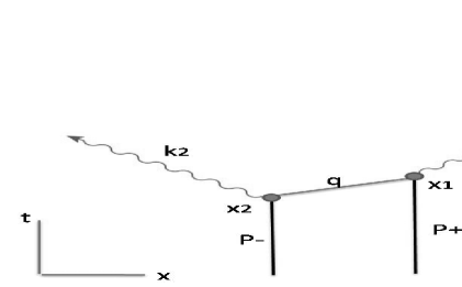
Figure 1: A two photon Feynman diagram. An electron, $p_{-},$ emits a photon, $k_{2},$ while scattering to a virtual state, $q$. It then annihilates with a positron, $p_{+}$, while creating a second photon, $k_{1}.$

II.1 Positron annihilation

Position annihilation according to the Dirac equation is discussed by Sakurai. He performs a perturbation expansion in powers of $e$ and finds that the first nonzero term is of second order. The Feynman diagram of such a process is sketched in Fig. 1: An electron with four-momentum $p_{-}=\left(E_{-},\mathbf{p}_{-}\right)$ is scattered to four-momentum $q=\left(q_{0},\mathbf{q}\right)$ at space-time point $x_{2}=\left(t_{2},\mathbf{x}_{2}\right)$ while emitting a photon with four-momentum $k_{2}=\left(\omega_{2},\mathbf{k}_{2}\right).$ At $x_{1}$ this electron annihilates with the positron and emits a photon with four-momentum $k_{1}.$ If instead the positron is scattered first, $q\leftrightarrow-q$ and the photons are interchanged. Sakurai obtains a scattering cross section for two-photon annihilation of $\pi r_{0}^{2}/\beta_{+}$ where $r_{0}=\alpha/m$. The Bohr radius, $a_{0}=1/\left(\alpha m\right)$, is larger than $r_{0}$ by a factor $\alpha^{-2}$, so the volume of an atom appears infinite on the length scale $r_{0}$ and the center of energy momentum is conserved, that is

$$\mathbf{k}_{1}+\mathbf{k}_{2}=\mathbf{p}_{+}+\mathbf{p}_{-}.$$ (1)

Sakurai applies his scattering theory to Ps by setting the electron density equal to $\left|\psi_{1s}\right|^{2}=1/\left[\pi\left(2a_{0}\right)^{3}\right]$ and obtains a decay rate

$$\Gamma=\frac{1}{2}\alpha^{5}m,$$ (2)

equivalent to a lifetime $\Gamma^{-1}=125\ ps$.

In Sakurai’s covariant formulation energy and momentum are conserved at the vertices and the state $q$ describes a virtual particle for which the Fermion dispersion relation is not imposed. However, since the final and initial states describe real particles, the dispersion relations

$$\omega_{j} =\left|\mathbf{k}_{j}\right|,$$ (3)

$$E_{\pm} =\sqrt{m^{2}+\left|\mathbf{p}_{\pm}\right|^{2}}$$

must be satisfied. In the more usual noncovariant formulation of perturbation theory, the dispersion relation is satisfied by the virtual Fermion but energy is not conserved between $t_{1}$ and $t_{2}$. To zero order in $\beta_{\pm}$ the annihilation photon $k_{2}$ has energy $m$, so the excess energy of the virtual state must be greater than $m$. Thus the intermediate state in Fig. 1 persists for less than $m^{-1}=1.3\times 10^{-21}\ s,$ implying that two photon annihilation is effectively instantaneous.

II.2 Relative and center coordinates

Here the center (of energy) and relative coordinates,

$$\mathbf{k}_{c} =\mathbf{k}_{1}+\mathbf{k}_{2},\ \mathbf{k}_{r}=\frac{1}{2}\left(\mathbf{k}_{1}-\mathbf{k}_{2}\right),$$ (4)

$$\mathbf{p}_{c} =\mathbf{p}_{+}+\mathbf{p}_{-},\ \ \mathbf{p}_{r}=\frac{1}{2}\left(\mathbf{p}_{+}-\mathbf{p}_{-}\right),\$$

$$\mathbf{x}_{c} =\frac{1}{2}\left(\mathbf{x}_{1}+\mathbf{x}_{2}\right),\ \text{and }\mathbf{x}_{r}=\mathbf{x}_{1}-\mathbf{x}_{2},$$

will be used. Since $\mathbf{k}_{1}\cdot\mathbf{x}_{1}+\mathbf{k}_{2}\cdot\mathbf{x}_{2}=\mathbf{k}_{c}\cdot\mathbf{x}_{c}+\mathbf{k}_{r}\cdot\mathbf{x}_{r}$ for the photons and $\mathbf{p}_{+}\cdot\mathbf{x}_{1}+\mathbf{p}_{-}\cdot\mathbf{x}_{2}=\mathbf{p}_{c}\cdot\mathbf{x}_{c}+\mathbf{p}_{r}\cdot\mathbf{x}_{r}$ for the Fermions, the exponent in a Fourier transform is preserved by this transformation, and relative momentum and position are conjugate observables, as are center momentum and position.

For counterpropagating photons the magnitudes of $\mathbf{k}_{1}$ and $\mathbf{k}_{2}$ should be added (subtracted) to obtain the magnitude of the relative (center) wave vector so that, according to (3) and (4),

$$\omega \equiv\omega_{1}+\omega_{2}=2\left|\mathbf{k}_{r}\right|,$$ (5)

$$\Delta\omega \equiv\omega_{1}-\omega_{2}=\left|\mathbf{k}_{c}\right|.$$

To second order in $\beta_{\pm}$ the Ps total energy is

$$E=2m+p_{c}^{2}/4m.$$ (6)

For a positron created at time $t_{0}$ contributions with different $p_{c}$ rapidly get out of phase due to the factor $\exp\left[-ip_{c}^{2}\left(t-t_{0}\right)/4m\right]$, leading to a density matrix that is diagonal in center of energy momentum. The relative dynamics, described by $\mathbf{k}_{r}$, is decoupled from the center motion, described by $\mathbf{k}_{c}$. In relative and center coordinates conservation of momentum, (1), becomes

$$\mathbf{k}_{c}=\mathbf{p}_{c}.$$ (7)

Since $\mathbf{p}_{c}$ has a definite value, the momenta of the annihilation photons are maximally restricted according $\mathbf{k}_{2}=\mathbf{p}_{c}-\mathbf{k}_{1}$ as observed by Irby.

II.3 Dynamics

Sakurai calculates the Ps decay rate so, implicitly, $\omega$ isn’t exactly equal to $E,$ but has a linewidth, $\Gamma$. Decay as a function of $t$ will be considered in this subsection.

A pure state will be written as a linear combination of a Ps atom in the $1s$ state with definite center of mass momentum $\mathbf{p}_{c}$, and the two annihilation photons described by their relative and center momenta. If a positron is injected at time $t_{0}$ the Schrödinger picture (SP) state vector is then

$$\left|\Psi_{\mathbf{k}_{c}}\right\rangle=c_{1s}\left(t\right)\left|1s,\mathbf{k}_{c}\right\rangle+\sum_{\mathbf{k}_{r}}c_{\mathbf{k}_{r}}\left(t\right)\left|\mathbf{k}_{r},\mathbf{k}_{c}\right\rangle.$$ (8)

for $t>t_{0}$ and $\left|\Psi_{\mathbf{k}_{c}}\right\rangle=0$ for $t<t_{0}$. We will take the volume, $V$, to be finite so that the momenta are discrete. To second order in $e$ the dynamical equations describing the relative motion for $t>t_{0}$ are SakuraiPage184

$$\overset{\cdot}{c_{1s}}\left(t\right) =-iEc_{1s}\left(t\right)-i\sum_{\mathbf{k}_{r}}\ U_{r}^{(2)}c_{\mathbf{k}_{r}}\left(t\right),$$ (9)

$$\overset{\cdot}{c}_{\mathbf{k}_{r}}\left(t\right) =-i\omega c_{\mathbf{k}_{r}}\left(t\right)-iU_{r}^{(2)}\ c_{1s}\left(t\right)$$

where the dot denotes differentiation with respect to $t$ and $\overset{\cdot}{U}_{fi}^{(2)}=U_{r}^{(2)}\delta^{3}\left(\mathbf{k}_{c}-\mathbf{p}_{c}\right)$ is the time derivative of the transition matrix element from Ps to the two-photon state. Eqs. (9) describe Weisskopf-Wigner spontaneous emission that is exponential in time and Lorentzian in frequency. A system of equations of the form (9) are solved in the interaction picture in Scully . For $t-t_{0}\gg\Gamma^{-1}$ decay is essentially complete so that the photon pulse is well separated from the source and ScullyEq18 gives

$$c_{\mathbf{k}_{r}}\left(t\right)=AU_{r}^{(2)}\frac{\exp\left[-i\omega\left(t-t_{0}\right)\right]}{\omega-E+i\Gamma}$$ (10)

in the SP with $\omega=2\left|\mathbf{k}_{r}\right|$ and $E=2m$ to first order in $\beta_{\pm}$. The factor $A$ is a constant and (10) can be normalized using the integral $I1$ in Appendix A with the result

$$c_{\mathbf{k}_{r}}\left(t\right)=\sqrt{\frac{8\pi\Gamma}{VE^{2}}}\frac{\exp\left[-i\omega\left(t-t_{0}\right)\right]}{\omega-E+i\Gamma}.$$ (11)

A pure state vector is of the form

$$\left|\Psi_{\mathbf{k}_{c}}\right\rangle=\Theta\left(\tau_{1}-t_{0}\right)\Theta\left(\tau_{2}-t_{0}\right)\left|\mathbf{k}_{c}\right\rangle\otimes\left|\Psi_{r}\right\rangle$$ (12)

$$\tau_{j}\equiv t-\left|\mathbf{x}_{j}\right|$$ (13)

where $\mathbf{x}_{j}$ is the position of the $j^{th}$ photon, $\tau_{j}$ is its emission time, the $\Theta$-functions ensure that no photons exist before the positron is injected, and

$$\left|\Psi_{r}\right\rangle=\sqrt{\frac{8\pi\Gamma}{VE^{2}}}\sum_{\mathbf{k}_{r}}\frac{\exp\left[-i\omega\left(t-t_{0}\right)\right]}{\omega-E+i\Gamma}\left|\mathbf{k}_{r}\right\rangle$$ (14)

describes the relative dynamics.

The space-time wave function is $\psi\left(\mathbf{x}_{r},t\right)=\left\langle\mathbf{x}_{r}|\Psi_{r}\right\rangle$ such that

$$\left|\Psi_{r}\right\rangle=\int d^{3}x_{r}\psi\left(\mathbf{x}_{r},t\right)\left|\mathbf{x}_{r}\right\rangle$$ (15)

with

$$\psi\left(\mathbf{x}_{r},t\right) =\sqrt{\frac{4\Gamma}{E^{2}}}\sum_{\mathbf{k}_{r}}\frac{\exp\left(i\omega t_{0}\right)}{\omega-E+i\Gamma}$$ (16)

$$\times\frac{\exp\left(i\mathbf{k}_{r}\cdot\mathbf{x}_{r}-i\omega t\right)}{\left(2\pi\right)^{3/2}}.$$

Strictly speaking, the $\mathbf{k}_{r}$-amplitudes should be weighted as in a $1s$ state, but $\Gamma\ll a_{0}^{-1}$, so this can be ignored. Substitution of $\mathbf{k}=\mathbf{k}_{r}$, $\mathbf{r}=\mathbf{x}_{r}$ and $t=t-t_{0}$ in integral $I2$ of in Appendix B gives

$$\psi\left(\left|\mathbf{x}_{r}\right|,t\right) =\sqrt{\frac{\Gamma}{4\pi}}\frac{1}{\left|\mathbf{x}_{r}\right|}$$ (17)

$$\times\exp\left[-\left(iE+\Gamma\right)\left(t-t_{0}-\frac{1}{2}\left|\mathbf{x}_{r}\right|\right)\right]$$

where a similar term involving $t-t_{0}+\frac{1}{2}\left|\mathbf{x}_{r}\right|$ has been neglected. This wave function is normalized if it is assumed that the photon pulse has propagated far enough so that $\exp\left[-\Gamma\left(t-t_{0}\right)\right]\ll 1$.

For a measurement described by the operator $\widehat{O}$, the expected value is

$$\left\langle\widehat{O}\right\rangle=\sum_{\mathbf{k}_{c}}p_{\mathbf{k}_{c}}\left\langle\Psi_{\mathbf{k}_{c}}\left|\widehat{O}\right|\Psi_{\mathbf{k}_{c}}\right\rangle.$$ (18)

where $\left|\Psi_{\mathbf{k}_{c}}\right\rangle$ given by (12) is a pure state and the probability for center of mass momentum $\mathbf{k}_{c}$ is $p_{\mathbf{k}_{c}}$. Normalization is such that $\left\langle\mathbf{x}_{r}|\mathbf{x}_{r}^{\prime}\right\rangle=\delta^{3}\left(\mathbf{x}_{r}-\mathbf{x}_{r}^{\prime}\right),$ $\left\langle\mathbf{k}_{c}|\mathbf{k}_{c}^{\prime}\right\rangle=\delta_{\mathbf{k}_{c},\mathbf{k}_{c}^{\prime}}$ and $\sum_{\mathbf{k}_{c}}p_{\mathbf{k}_{c}}=\sum_{\mathbf{k}_{r}}\left|c_{\mathbf{k}_{r}}\right|^{2}=$ $\int d^{3}x_{r}\left|\psi\left(\mathbf{x}_{r},t\right)\right|^{2}=1$. The $\Theta$-functions in (12) limit the volume that the $j^{th}$ photon can occupy to $V=\frac{4}{3}\pi\left(t-t_{0}\right)^{3}$. For finite volume conservation of momentum, (7), is approximate, with uncertainty of order $\pi/\left(t-t_{0}\right)$ in each of its components.

III Application to experiments

In this Section, Eq. (18) will be applied to Doppler broadening (PAS experiments) and the arrival time difference between the nuclear photon and one of the annihilation photons (PAL experiments), and the Irby experiment will be analyzed.

III.1 Doppler broadening

Ref. Shibuya reports measurement of the distribution of the Ps center of mass momentum, so that $\widehat{O}=\left|\mathbf{k}_{c}\right\rangle\left\langle\mathbf{k}_{c}\right|$. Substitution in (18) gives the probability of center wave vector $\mathbf{k}_{c}$ as

$$\left\langle\left|\mathbf{k}_{c}\right\rangle\left\langle\mathbf{k}_{c}\right|\right\rangle=p_{\mathbf{k}_{c}}.$$ (19)

This experiment was performed using a positron source embedded in biological tissue, and the Gaussian distribution

$$p\left(\mathbf{k}_{c}\right)=\frac{1}{\left(\pi\sigma^{2}\right)^{3/2}}\exp\left(-\frac{\left|\mathbf{k}_{c}\right|^{2}}{\sigma^{2}}\right)$$ (20)

with $\sigma=2.4keV=0.005m$ was obtained. The continuous distribution in related to the discrete probability by $p\left(\mathbf{k}\right)=p_{\mathbf{k}_{c}}V/\left(2\pi\right)^{3}.$

If these center of mass momenta were to add coherently, the time uncertainty for the second photodetection event would be very small. However, the photon momenta are maximally correlated so, if $\mathbf{x}_{c}$ were to be measured, (18) gives

$$\left\langle\left|\mathbf{x}_{c}\right\rangle\left\langle\mathbf{x}_{c}\right|\right\rangle=\sum_{\mathbf{k}_{c}}p_{\mathbf{k}_{c}}\left|\left\langle\mathbf{x}_{c}|\mathbf{k}_{c}\right\rangle\right|^{2}=\frac{1}{V}.$$ (21)

This implies that the photon center of energy is equally likely to be found anywhere within the allowed volume, since the only information available about its position is a consequence of causality and knowledge of the position and time of positron injection.

III.2 PAL experiments

In PAL experiments such as the measurement of positron lifetime in $\alpha$-$\operatorname{Si}$O₂ Saito , photons are counted at fixed $\mathbf{x}_{1}$ as a function $t-t_{0}$. It is assumed here that para-Ps forms as soon as the positron is injected, although in reality the situation is more complicated than this. To first order in $\beta_{\pm}$ the wave vector $\mathbf{k}_{r}$ has length $m$ and arbitrary direction. The wave vector $\mathbf{k}_{c}$ has a definite value and its magnitude is distributed according to (20). Substitution of $\widehat{O}=\left|\mathbf{x}_{1}\right\rangle\left\langle\mathbf{x}_{1}\right|,$ $\widehat{1}=\int d^{3}x_{2}\left|\mathbf{x}_{2}\right\rangle\left\langle\mathbf{x}_{2}\right|$, (12), and (17) in (18) gives

$$\left\langle\left|\mathbf{x}_{1}\right\rangle\left\langle\mathbf{x}_{1}\right|\right\rangle =\frac{\Gamma}{4\pi V}\exp\left[-\Gamma\left(t-t_{0}\right)\right]$$ (22)

$$\times\Theta\left(t-t_{0}-\left|\mathbf{x}_{1}\right|\right)$$

$$\times\int d^{3}x_{2}\Theta\left(t-t_{0}-\left|\mathbf{x}_{2}\right|\right)$$

$$\times\left|\mathbf{x}_{r}\right|^{-2}\exp\left[-\Gamma\left(t-t_{0}-\left|\mathbf{x}_{r}\right|\right)\right].$$

This is just the trace of the density matrix over the unobserved second photon. If the $z$-axis is chosen parallel to $\mathbf{k}_{1}$, the distribution of $\mathbf{k}_{2}$ values is centered at $\theta=\pi$ and the factor $\exp\left(\Gamma\left|\mathbf{x}_{r}\right|\right)$ selects solid angle $\Omega$ determined by $\Gamma$ and centered about $\cos\theta=-1$. To first order in $\beta_{\pm}$

$$\left|\mathbf{x}_{r}\right|=\left|\mathbf{x}_{1}\right|+\left|\mathbf{x}_{2}\right|.$$ (23)

In the limit $\left|\mathbf{x}_{1}\right|\gg\Gamma^{-1},$ consistent with our assumption that the pulse is well separated from the source, $\left|\mathbf{x}_{r}\right|\approx 2\left|\mathbf{x}_{2}\right|$ and the probability density to count a photon at $\mathbf{x}_{1}$ a time $t-t_{0}$ after positron injection reduces to

$$\left\langle\left|\mathbf{x}_{1}\right\rangle\left\langle\mathbf{x}_{1}\right|\right\rangle =\frac{\Omega}{16\pi V}\exp\left[-\Gamma\left(t-t_{0}-\left|\mathbf{x}_{1}\right|\right)\right]$$ (24)

$$\times\Theta\left(t-t_{0}-\left|\mathbf{x}_{1}\right|\right)$$

where $V=\frac{4}{3}\pi\left(t-t_{0}\right)^{3}$. Thus the rate at which correlated nuclear and annihilation photons are counted decays exponentially. The coefficient of the exponential reflects our limited knowledge of the position of the two-photon center of energy.

III.3 Irby experiment

In the Irby experiment, illustrated in Fig. 2, photons are emitted by a source, $S,$ approximately $3mm$ thick. They are detected at the fixed positions $\mathbf{x}_{1}$ and $\mathbf{x}_{2}$ as a function of $t_{1}-t_{2}$ where $t_{j}$ is the time when a photon is counted at detector $j$. Irby derived a wave function that generalizes the example considered by Einstein, Podolsky and Rosen (EPR) by including time dependence and conservation of energy IrbyTheory . He assumed zero center of mass motion so that the photons have momentum $p$ and $-p$. The relative position, $\mathbf{x}_{r}$, corresponds to $x_{1}-x_{2}$ and the Fourier amplitude, $c_{\mathbf{k}_{r}},$ given by (11) corresponds to $f\left(p\right)$ in Irby’s Eq. (13).

Following EPR and Irby EPR ; IrbyTheory and using (23) in the form $\left|\mathbf{x}_{r}\right|=\left|\mathbf{x}_{<}\right|+\left|\mathbf{x}_{>}\right|$, the wave function (17) can be written as

$$\psi\left(\left|\mathbf{x}_{r}\right|,t\right)=\int_{0}^{\infty}dx\delta\left(\left|\mathbf{x}_{<}\right|-x\right)\psi\left(\left|\mathbf{x}_{>}\right|+x,t\right)$$ (25)

where $\delta\left(\left|\mathbf{x}_{<}\right|-x\right)$ is a positon eigenvector with eigenvalue $x$, $\mathbf{x}_{<}\$is the position while $t_{<}$ is the time of the first photodetection event, and $\mathbf{x}_{>}$ is the position of the second photon. When the first photon is counted at time $t_{<}$ the wave function collapses to the coefficient of the $\delta$-function in (25). To ensure propagation at the speed of light this one-photon exponentially decaying pulse can be written as

$$\psi\left(\left|\mathbf{x}_{>}\right|,t\right) =\sqrt{\frac{\Gamma}{4\pi}}\frac{1}{\left|\mathbf{x}_{<}\right|+\left|\mathbf{x}_{>}\right|}$$ (26)

$$\times\exp\left[-\frac{1}{2}\left(iE+\Gamma\right)\left(t_{<}-t_{0}-\left|\mathbf{x}_{<}\right|\right)\right]$$

$$\times\exp\left[-\frac{1}{2}\left(iE+\Gamma\right)\left(t-t_{0}-\left|\mathbf{x}_{>}\right|\right)\right].$$

Time and distance dependence for the undetected photon is described by the last exponential, so the probability density is proportional to $\exp\left[-\Gamma\left(t-t_{0}-\left|\mathbf{x}_{>}\right|\right)\right]$ or zero. If the second photon is counted at time $t_{>}$, allowing for the $\mathbf{x}_{c}$ density $V^{-1}$ the probability density for coincident photodetection is

$$P=\frac{1}{V}\left|\psi\left(\left|\mathbf{x}_{r}\right|,\frac{t_{1}+t_{2}}{2}\right)\right|^{2}$$ (27)

where $\left|\mathbf{x}_{r}\right|$ is the detector separation, $t_{<}+t_{>}=t_{1}+t_{2}$ and $\psi$ is given by (17).

Essentially the same result is obtained from the second order Glauber correlation function Glauber ,

$$G^{(2)}\left(x_{1},x_{2}\right)=\left\langle E^{(-)}\left(x_{1}\right)E^{(-)}\left(x_{2}\right)E^{(+)}\left(x_{2}\right)E^{(+)}\left(x_{1}\right)\right\rangle$$ (28)

where $x_{j}=\left(t_{j},\mathbf{x}_{j}\right)$. For photodetection at times $t_{1}$ and $t_{2}$, the positive frequency electric field operators in $G^{(2)}$ result in a factor

$$\exp\left[-i\left(\omega_{1}t_{1}+\omega_{2}t_{2}\right)\right] =\exp\left[-i\left(\omega\frac{t_{1}+t_{2}}{2}\right.\right.$$ (29)

$$\left.\left.+\frac{\Delta\omega}{2}\left(t_{1}-t_{2}\right)\right)\right]\text{.}$$

Since $\sqrt{\omega_{1}\omega_{2}}=m$ is a constant to first order in $\beta_{\pm}$,

$$G^{(2)}\left(x_{1},x_{2}\right)\propto\frac{1}{V}\left|\psi\left(\left|\mathbf{x}_{r}\right|,\frac{t_{1}+t_{2}}{2}\right)\right|^{2}$$ (30)

equal to $P$ given by (27).

The probability density $P$ is proportional to $\exp\left[-\Gamma\left(t_{1}+t_{2}-2t_{0}\right)\right]$, but Irby measured the distribution of $t_{1}-t_{2}$, and neither (27) nor the absolute square or Irby’s wave function in IrbyExpt gives their probabilities directly. The resolution to this problem lies in averaging over the positron injection time, $t_{0}$, that is not measured but must be earlier than both $\tau_{1}$ and $\tau_{2}$. If it is assumed that positrons are injected at a constant rate $r=1/T$ , substitution of (17) in (27) gives

$$P =\frac{r\Gamma}{4\pi\left|\mathbf{x}_{r}\right|^{2}V}\int_{-T/2}^{T/2}dt_{0}$$ (31)

$$\times\exp\left[-\Gamma\left(t_{1}+t_{2}-2t_{0}-\left|\mathbf{x}_{r}\right|\right)\right]$$

$$\times\Theta\left(\tau_{1}-t_{0}\right)\Theta\left(\tau_{2}-t_{0}\right).$$

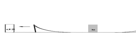
Figure 2: Irby experiment. A positron is created in the source, S, and the time difference between annihilation photons arriving at detectors d1 and d2 is measured.

The integral (31) is evaluated as $I3$ in Appendix C with the upper limit of the $t_{0}$ integral is taken to be the earlier photon emission time. The result is

$$P=\frac{r}{8\pi\left|\mathbf{x}_{r}\right|^{2}V}\exp\left(-\Gamma\left|\tau_{1}-\tau_{2}\right|\right),$$ (32)

where $\tau_{j}=t_{j}-\left|\mathbf{x}_{j}\right|$.

Irby fit his date to a Lorentzian curve while, according to (32), the experimental picosecond timing analyzer (PTA) spectrum in Figs. 4 and 5 of Ref. IrbyExpt is a double exponential. This discrepancy is addressed in Fig. 3 that shows a comparison of a double exponential to a Lorentzian and a Gaussian. The double exponential gives the sharp peaks observed by Irby while behaving like the Lorentzian that he used in his fits in the tails. The Gaussian has an appreciably different shape and does not fit the data as noted by Irby. Eq. (32) derived here should give an improved description of the experimental results.

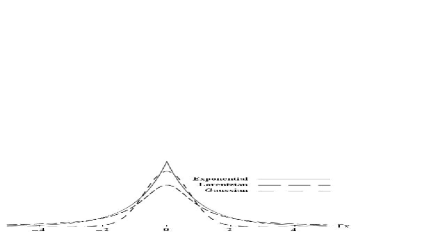
Figure 3: Comparison of exponential of the absolute value, $\left(2\Gamma\right)^{-1}\exp\left(-\Gamma\left|x\right|\right)$ with a Lorentzian, $\left(\pi\Gamma^{2}\right)^{-1}\left(x^{2}+\Gamma^{2}\right)^{-1},$ and a Gaussian, $\left(\Gamma\pi\right)^{-3/2}\exp\left(-\Gamma^{2}x^{2}\right)$.

IV Conclusion

This paragraph describes the details of the present calculation in relation to the previous theoretical work: In Refs. EPR and IrbyTheory the center of energy momentum is set equal to zero, the wave function is given as a function of the relative coordinates, and the time during which the photons interact, here $t_{0}$ to $t_{0}+\Gamma^{-1}$, is assumed to be known. In the present calculation the momentum of the center of energy has a wide range of definite values consistent with the PAS experiments, and the positron injection time is unknown. In EPR all relative momenta are given equal weight. Since the time when the particles interact is known, when one of the counterpropagating photons is detected the position of the second photon is determined exactly and nonlocally by collapse of the wave function. Here and in IrbyTheory the relative momenta, $p=\left|\mathbf{k}_{r}\right|$, are restricted by a function $f\left(p\right)$ which we find here is a Lorentzian with center at $\left|\mathbf{k}_{r}\right|=m$ and FWHM $2\Gamma$, resulting in exponential decay in space-time.

Irby attributed the unexpectedly wide range of annihilation photon PTA detection time differences that he observed to maximally restricted photon momenta, leading to the elimination of nonlocality in the conjugate position observables IrbyTheory . Here the pure states have definite center of energy momentum and Ps decay is described in terms of the relative coordinates. After averaging over the unobserved positron injection time, the annihilation photon coincidence rate was found to be proportional to $\exp\left(-\Gamma\left|\tau_{1}-\tau_{2}\right|\right)$ where $\tau_{j}$ is the photon emission time. This supports Irby’s observation IrbyExpt that annihilation photon pulse width is limited by the Ps lifetime. Only the peak of the double exponential function is determined by the position of the positron source. This is counter to expectations, and should be taken into account in TOF PET imaging.

Annihilation photons have played a significant role in the development of our understanding of quantum correlations. Their polarization correlations were considered, and discarded, as a candidate for the first experimentally realizable test of Bell’s theorem Bell . EPR used position correlations of a pair of counterpropagating particles as their primary example of nonlocal collapse EPR . Irby performed a direct measurement of annihilation photon space-time correlations and concluded that their nonlocality is erased by maximal restriction of their momenta. Here we find that their momenta are maximally correlated because their center of energy momentum has a well defined value. Position entanglement is ascribed to the relative coordinates, augmented by causality. The observed $123\ ps$ pulse width is attributed to uncertainty in the time of photon pair creation due to Ps annihilation.

Appendix A Relative normalization

Normalization requires evaluation of

$$I1=\sum_{\mathbf{k}}\frac{1}{\left(\omega-E\right)^{2}+\Gamma^{2}}=\frac{V}{2\pi^{2}}\int_{0}^{\infty}dkk^{2}\frac{1}{\left(\omega-E\right)^{2}+\Gamma^{2}}.$$

Since $\omega_{c}\approx 2\left|\mathbf{k}_{r}\right|$ according to (5), we want $\omega=2k$. Making a change of variables to $\eta=2k-E$ with limits $-\infty$ to $\infty$ and selecting a contour that encloses the pole at $\eta=-i\Gamma$ with $\Gamma\ll E$ gives

$$I1=\frac{V}{2\pi^{2}}\left(\frac{E}{2}\right)^{2}\frac{2\pi i}{4i\Gamma}=\frac{VE^{2}}{16\pi\Gamma}.$$

Appendix B Relative k- to x-space integral

To evaluate (16) we need

$$I2 =\sqrt{\frac{16\pi\Gamma}{V^{2}E^{2}}}\int d^{3}k\frac{\exp\left(i\mathbf{k}\cdot\mathbf{r}-i\omega t\right)}{\omega-E+i\Gamma}$$

$$=\sqrt{\frac{16\pi\Gamma}{E^{2}}}\frac{2\pi}{ir}\int_{0}^{\infty}dkk\frac{\exp\left(ikr\right)-\exp\left(-ikr\right)}{2k-E+i\Gamma}$$

$$\times\exp\left(-i2kt\right).$$

$$=\sqrt{\frac{\Gamma}{4\pi}}\frac{1\ }{r}\left\{\exp\left[-\left(iE+\Gamma/2\right)\left(t-\frac{1}{2}r\right)\right]\right.$$

$$\left.-\exp\left[-\left(iE+\Gamma\right)\left(t+\frac{1}{2}r\right)\right]\right\}$$

Appendix C Irby experiment $t_{0}$-integral

We need

$$I3 =\int_{-T/2}^{T/2}dt_{0}\exp\left[-\Gamma\left(2t_{c}-2t_{0}-\left|\mathbf{x}_{r}\right|\right)\right]$$

$$\times\Theta\left(\tau_{1}-t_{0}\right)\Theta\left(\tau_{2}-t_{0}\right)$$

If $T\gg\Gamma^{-1}$ the limits can be extended to $\pm\infty$ and the $\Theta$-functions imply that

$$I3 =\exp\left[-\Gamma\left(2t_{c}-\left|\mathbf{x}_{r}\right|\right)\right]\int_{-\infty}^{\tau_{<}}dt_{0}\exp\left[2\Gamma t_{0}\right]$$

$$=\left(2\Gamma\right)^{-1}\exp\left[-\Gamma\left(2t_{c}-2\tau_{<}-\left|\mathbf{x}_{r}\right|\right)\right]$$

where $\tau_{>}$ $(\tau_{<})$ is the larger (smaller) of $\tau_{1}$ and $\tau_{2}.$ Since according to (4) and (13)

$$2t_{c}-2\tau_{<} =t_{>}+t_{<}-2t_{<}+2\left|\mathbf{x}_{<}\right|$$

$$=t_{>}-t_{<}+2\left|\mathbf{x}_{<}\right|,$$

$$I3=\left(2\Gamma\right)^{-1}\exp\left[-\Gamma\left(t_{>}-t_{<}-\left|\mathbf{x}_{r}\right|+2\left|\mathbf{x}_{<}\right|\right)\right].$$

Eq. (23) gives $\left|\mathbf{x}_{r}\right|=\left|\mathbf{x}_{>}\right|+\left|\mathbf{x}_{<}\right|$, that is the distance between the detectors equals the sum of the source-detector distances, so that

$$I3 =\left(2\Gamma\right)^{-1}\exp\left[-\Gamma\left(t_{>}-t_{<}-\mathbf{x}_{>}+\left|\mathbf{x}_{<}\right|\right)\right]$$

$$=\left(2\Gamma\right)^{-1}\exp\left[-\Gamma\left(\tau_{>}-\tau_{<}\right)\right].$$

References

• (1) V. I. Grafutin and E. P. Prokop’ev, Physics-Uspekhi Rev. 45, 59 (2002).
• (2) H. Saito and T. Hyodo, Phys. Rev. Lett. 90, 193401 (2003).
• (3) T. K. Lewellen, Seminars in Nuclear Medicine 28, 268 (1998).
• (4) V. D. Irby, Meas. Sci. Technol. 15, 1799 (2004).
• (5) A. Einstein, B. Podolsky and N. Rosen, Phys. Rev. 47 , 777 (1935).
• (6) V. D. Irby, Phys. Rev A 67, 034102 (2003).
• (7) J. J. Sakurai, Advanced Quantum Mechanics (Addison-Wesley, 1967).
• (8) Ref. Sakurai , pp. 40 and 183.
• (9) M. O. Scully and M. S. Zubairy, Quantum Optics (Cambridge Univ. Press, 1997).
• (10) Ref. Scully , Eq. (6.3.18).
• (11) K. Shibuya, EW. Yoshida, F. Nishikido, T. Suzuki, T. Tsuda, N. Inadama, T. Yamaya and H. Murayama, IFMBE Proceedings 14, 1667 (2006).
• (12) R. J. Glauber, Phys. Rev. 130, 2529 (1963).
• (13) J. F. Clauser, M. A. Horne, A. Shimony, and R. A. Holt, Phys. Rev. Lett. 23, 880 (1969).