Entanglement evolution in multipartite cavity-reservoir systems under local unitary operations

Abstract

We analyze the entanglement evolution of two cavity photons being affected by the dissipation of two individual reservoirs. Under an arbitrary local unitary operation on the initial state, it is shown that there is only one parameter which changes the entanglement dynamics. For the bipartite subsystems, we show that the entanglement of the cavity photons is correlated with that of the reservoirs, although the local operation can delay the time at which the photon entanglement disappears and advance the time at which the reservoir entanglement appears. Furthermore, via a new defined four-qubit entanglement measure and two three-qubit entanglement measures, we study the multipartite entanglement evolution in the composite system, which allows us to analyze quantitatively both bipartite and multipartite entanglement within a unified framework. In addition, we also discuss the entanglement evolution with an arbitrary initial state.

I Introduction

As one of the most subtle phenomena in many-body systems, quantum entanglement has now been an important physical resource widely used in quantum communication and quantum computation hor09rev ; ple07qic . Therefore it is fundamental to characterize the entanglement nature in quantum systems, especially at a quantitative level. Till now, although bipartite entanglement is well understood in many aspects, the entanglement in multipartite systems is far from clear and thus deserve further exploration.

Entanglement dynamical behavior is an important property in practical quantum information processing. This is because entanglement is fragile and always decays due to unwanted interactions between the system and its environment. A theoretical study of two-atom spontaneous emission shows that entanglement does not always decay in an asymptotic way and it can be corrupted in a finite time tyu04prl , which is referred to as entanglement sudden death (ESD). Some earlier studies also pointed out this fact that even a very weakly dissipative environment can disentangle the quantum system in a finite time zyc01pra ; akr01pra ; daf03pra ; dod04pra . The ESD phenomenon has recently received a lot of attentions ban06jpa ; san06pra ; der06pra ; sun07pra ; lfw09pra ; fan09pra ; ajh10pra ; ysw10pra (see also a review paper tyu09sci and references therein), and, experimentally, it has been detected in photon alm07sci and atom systems lau07prl .

A deep understanding on the ESD phenomenon concerns the problem where the lost entanglement goes. To answer the question, it is proper to enlarge the system to include its environment. Recently, López et al analyzed the entanglement evolution in a composite system consisting of entangled cavity photons with individual reservoirs clo08prl , and show that the entanglement sudden birth (ESB) of reservoir-reservoir subsystem must happen whenever the ESD of cavity-cavity subsystem occurs. Moreover, in Ref. byw09pra , Bai et al presented a entanglement monogamy relation in multipartite systems and analyzed quantitatively the bipartite entanglement transfer in the multipartite cavity-reservoir system.

However, in the above analysis, the multipartite entanglement in the composite cavity-reservoir system is not well characterized, although the residual entanglement byw09pra can indicate its existence. Moreover, the authors only consider the symmetric initial state like $|\phi\rangle=\alpha|00\rangle+\beta|11\rangle$. When the initial state is asymmetric, the entanglement evolution can be very different. For example, a $\sigma_{x}$ operation acting on the symmetric state can change the evolution of the entangled cavity photons from the ESD route to the asymptotic decay route, although the two kinds of initial states have the equal entanglement. Therefore, it is desirable to consider the entanglement dynamical behavior for the asymmetric case and, particularly, find a good entanglement measure to characterize the genuine multipartite entanglement evolution.

In this paper, for the asymmetric initial state modulated by an arbitrary local unitary (LU) operation, we analyze its entanglement evolution in the multipartite cavity-reservoir system. In Sec. II, we derive the effective output state under the LU operation, in which there is only one parameter affecting the entanglement dynamics. In Sec. III, we analyze the bipartite entanglement transfer in the composite system, and point out the cavity photon entanglement is still correlated with the reservoir entanglement although the local operation can delay the ESD time and advance the ESB time. In Sec. IV, the multipartite entanglement evolution is studied via a new defined four-qubit entanglement measure and two three-qubit entanglement measures. In Sec. V, within a unified framework, we investigate the relation between bipartite entanglement transfer and multipartite entanglement transition in the composite system. Finally, we discuss the entanglement evolution with an arbitrary initial state and give a brief conclusion in Sec. VI.

II The effective output state under the LU operation

Before the derivation of the effective output state under the LU operation, we first recall the multipartite cavity-reservoir system. In Ref. clo08prl , López et al considered two entangled cavity photons being affected by the dissipation of two individual $N$-mode reservoirs where the interaction of a single cavity-reservoir system is described by the Hamiltonian

$$\hat{H}=\hbar\omega\hat{a}^{\dagger}\hat{a}+\hbar\sum_{k=1}^{N}\omega_{k}\hat{b}_{k}^{\dagger}\hat{b}_{k}+\hbar\sum_{k=1}^{N}g_{k}(\hat{a}\hat{b}_{k}^{\dagger}+\hat{b}_{k}\hat{a}^{\dagger}).$$ (1)

The authors analyzed the entanglement evolution with the symmetric initial state

$$|\Phi_{0}\rangle=(\alpha|00\rangle+\beta|11\rangle)_{c_{1}c_{2}}|00\rangle_{r_{1}r_{2}},$$ (2)

in which the reservoirs are in the vacuum state and the quantum state of cavity photons is invariant under the permutation of the qubits $c_{1}$ and $c_{2}$. They show that, along the time evolution, the ESD of two photons can happen when the initial state amplitudes satisfy the condition $\alpha<\beta$, and this procedure is necessarily related to the ESB of two reservoirs.

Now, we consider the asymmetric initial state modulated by an arbitrary single-qubit LU operation. Without loss of generality, we assume that the operation acts on the first cavity, and then the initial state can be written as

$$|\Phi_{0}^{a}\rangle=U_{c_{1}}|\Phi_{0}\rangle.$$ (3)

For an arbitrary single qubit LU operation, one can decompose it as nie00book

$$U(\zeta,\eta,\gamma,\delta)=e^{i\zeta}R_{z}(\eta)R_{y}(\gamma)R_{z}(\delta),$$ (4)

where the $e^{i\zeta}$ is a global phase shift and $R_{k}(\theta)=\mbox{exp}(-i\theta\sigma_{k}/2)$ is the rotation along the $k(=y,z)$ axis with the $\sigma_{k}$ being the Pauli matrix. In this case, the output state under the time evolution is

$$|\Phi_{t}\rangle = U_{c_{1}r_{1}}(\hat{H},t)\otimes U_{c_{2}r_{2}}(\hat{H},t)|\Phi_{0}^{a}\rangle$$ (5)

$$\simeq U_{c_{1}r_{1}}(\hat{H}^{\prime},t)\otimes U_{c_{2}r_{2}}(\hat{H}^{\prime\prime},t)[R_{y}(\gamma)_{c_{1}}|\Phi_{0}\rangle],$$

where $\hat{H}^{\prime}=R_{z}^{\dagger}(\eta)_{c_{1}}\hat{H}R_{z}(\eta)_{c_{1}}$, $\hat{H}^{\prime\prime}=R_{z}^{\dagger}(\delta)_{c_{2}}\hat{H}R_{z}(\delta)_{c_{2}}$, and the $\simeq$ means the states on two sides are equivalent up to some LU operations (for a detail derivation, see the appendix). After considering the effect of the evolution $U_{c_{1}r_{1}}(\hat{H}^{\prime},t)$ on the entanglement dynamics, we find that it is equivalent to that of the evolution $U_{c_{1}r_{1}}(\hat{H},t)$ (in the appendix, we give the proof). The case for the evolution $U_{c_{2}r_{2}}(\hat{H}^{\prime\prime},t)$ is similar. Then Eq. (5) can be rewritten as

$$|\Phi_{t}\rangle\simeq U_{c_{1}r_{1}}(\hat{H},t)\otimes U_{c_{2}r_{2}}(\hat{H},t)[R_{y}(\gamma)_{c_{1}}|\Phi_{0}\rangle],$$ (6)

which means that, under an arbitrary LU operation $U_{c_{1}}(\zeta,\eta,\gamma,\delta)$, the entanglement evolution is only sensitive to the rotation $R_{y}(\gamma)_{c_{1}}$.

Therefore, the effective initial state for the entanglement evolution is

$$|\Psi_{0}\rangle=R_{y}(\gamma)_{c_{1}}|\Phi_{0}\rangle=(\alpha|\tilde{0}0\rangle+\beta|\tilde{1}1\rangle)_{c_{1}c_{2}}|00\rangle_{r_{1}r_{2}},$$ (7)

in which the new basic vectors are $|\tilde{0}\rangle=\mbox{cos}(\gamma/2)|0\rangle+\mbox{sin}(\gamma/2)|1\rangle$ and $|\tilde{1}\rangle=-\mbox{sin}(\gamma/2)|0\rangle+\mbox{cos}(\gamma/2)|1\rangle$. For the output state, we use the approximation clo08prl

$$U(\hat{H},t)_{cr}|10\rangle=\xi|10\rangle+\chi|01\rangle,$$ (8)

where the amplitudes are $\xi(t)=\mbox{exp}(-\kappa t/2)$ and $\chi(t)=[1-\mbox{exp}(-\kappa t)]^{1/2}$ in the limit of $N\rightarrow\infty$ for a reservoir with a flat spectrum. Then the effective output state has the form

$$|\Psi_{t}\rangle = \alpha(\mbox{cos}\frac{\gamma}{2}|00\rangle+\mbox{sin}\frac{\gamma}{2}|\phi_{t}\rangle)_{c_{1}r_{1}}|00\rangle_{c_{2}r_{2}}$$ (9)

$$-\beta(\mbox{sin}\frac{\gamma}{2}|00\rangle-\mbox{cos}\frac{\gamma}{2}|\phi_{t}\rangle)_{c_{1}r_{1}}|\phi_{t}\rangle_{c_{2}r_{2}},$$

where $|\phi_{t}\rangle=\xi(t)|10\rangle_{cr}+\chi(t)|01\rangle_{cr}$ and the parameter $\gamma$ being chosen in the range $[0,\pi]$.

III Two-qubit entanglement evolution under the LU operation

According to the effective output state $|\Psi_{t}\rangle$ in Eq. (9), we can derive the density matrices of different subsystems and analyze their entanglement dynamical behaviors. We first consider the subsystem of two cavity photons, for which its density matrix is

$$\rho_{c_{1}c_{2}}(t)=\psi_{1}+\psi_{2}+\psi_{3}+\psi_{4},$$ (10)

where $\psi_{i}=|\psi_{i}\rangle\langle\psi_{i}|$ and the four non-normalized pure state components are $|\psi_{1}\rangle=\alpha\mbox{cos}(\gamma/2)|00\rangle+\alpha\mbox{sin}(\gamma/2)\xi|10\rangle-\beta\mbox{sin}(\gamma/2)\xi|01\rangle+\beta\mbox{cos}(\gamma/2)\xi^{2}|11\rangle$, $|\psi_{2}\rangle=\beta\mbox{sin}(\gamma/2)\chi|00\rangle-\beta\mbox{cos}(\gamma/2)\xi\chi|10\rangle$, $|\psi_{3}\rangle=\alpha\mbox{sin}(\gamma/2)\chi|00\rangle+\beta\mbox{cos}(\gamma/2)\xi\chi|01\rangle$, and $|\psi_{4}\rangle=\beta\mbox{cos}(\gamma/2)\chi^{2}|00\rangle$, respectively. For the two reservoirs, its density matrix is similar to that of the cavity photons and the following relation holds

$$\rho_{r_{1}r_{2}}(t)=S_{\xi\leftrightarrow\chi}[\rho_{c_{1}c_{2}}(t)],$$ (11)

where $S_{\xi\leftrightarrow\chi}$ exchanges the parameters $\xi$ and $\chi$ (i.e., $\xi\rightarrow\chi$ and $\chi\rightarrow\xi$).

Based on the previous analysis in Ref. byw09pra , we choose the square of the concurrence to characterize the two-qubit entanglement evolution. The concurrence is defined as woo98prl $C(\rho_{ij})=\mbox{max}(0,\sqrt{\lambda_{1}}-\sqrt{\lambda_{2}}-\sqrt{\lambda_{3}}-\sqrt{\lambda_{4}})$ with the decreasing nonnegative real numbers $\lambda_{i}$ being the eigenvalues of the matrix $R_{ij}=\rho_{ij}(\sigma_{y}\otimes\sigma_{y})\rho_{ij}^{\ast}(\sigma_{y}\otimes\sigma_{y})$. After computing the eigenvalues of the matrices $R_{c_{1}c_{2}}$ and $R_{r_{1}r_{2}}$ expl2 , we can obtain

$$C_{c_{1}c_{2}}^{2}(t) = 4[\mbox{max}(|\alpha\beta\xi^{2}|-|\beta\xi\chi|^{2}\mbox{cos}^{2}(\gamma/2),0)]^{2},$$

$$C_{r_{1}r_{2}}^{2}(t) = 4[\mbox{max}(|\alpha\beta\chi^{2}|-|\beta\xi\chi|^{2}\mbox{cos}^{2}(\gamma/2),0)]^{2}.$$ (12)

Combining the concurrences and the expressions of $\xi(t)$ and $\chi(t)$ in Eq. (8), we know that, for a given asymmetric initial state (given the parameters $\alpha$, $\beta$ and $\gamma$), the cavity photons entanglement decreases and the reservoir entanglement increases along with the time evolution.

It is still an unsolved problem whether or not the ESD of cavity photons and the ESB of the reservoirs are correlated in the asymmetric case. With the conditions $C_{c_{1}c_{2}}(t)=0$ and $C_{r_{1}r_{2}}(t)=0$, we can deduce the times of the ESD and the ESB, which have the forms

$$t_{ESD}(\rho_{c_{1}c_{2}}) = -\frac{1}{\kappa}\mbox{ln}\left(1-\frac{\alpha}{\beta\cdot\mbox{cos}^{2}(\gamma/2)}\right),$$

$$t_{ESB}(\rho_{r_{1}r_{2}}) = \frac{1}{\kappa}\mbox{ln}\frac{\beta\cdot\mbox{cos}^{2}(\gamma/2)}{\alpha},$$ (13)

where the parameter $\kappa$ is the dissipative constant (note that $\xi=\mbox{exp}(-\kappa t/2)$ in the entanglement evolution). According to the two times, we can derive that the ESD of two photons occurs when $\beta\cdot\mbox{cos}^{2}(\gamma/2)>\alpha$, as is the case for the ESB of two reservoirs. This means that the correlation between the ESD and the ESB still holds for the asymmetric initial states, i.e., the ESB of the reservoirs must happen when the ESD of cavity photons occurs.

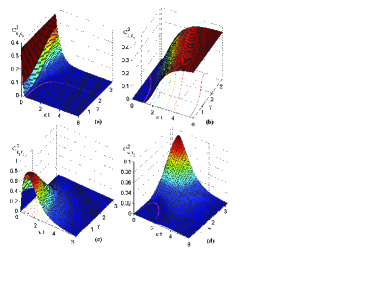
Figure 1: (Color online) Different two-qubit entanglement as a function of the time evolution $\kappa t$ and the rotation parameter $\gamma$.

As an example, we choose the initial state parameters as $\alpha=1/\sqrt{10}$ and $\beta=3/\sqrt{10}$. In Fig. 1(a), the concurrence $C_{c_{1}c_{2}}^{2}$ is plotted as a function of the time $\kappa t$ and the rotation parameter $\gamma$. For a fixed value of $\kappa t$, the photon entanglement increases with the parameter $\gamma$. When the $\gamma$ is given, the $C_{c_{1}c_{2}}^{2}$ decreases along the time $\kappa t$. The ESD line (the purple line) is also plotted in the figure, where the $\gamma$ can delay the ESD time. It is interesting that the entanglement evolution changes to the asymptotical decay route before the $\gamma$ attains to the value $\pi$, and the critical value is $\gamma=2\mbox{arccos}\sqrt{1/3}\approx 1.91063$. In Fig. 1(b), the entanglement evolution of $C_{r_{1}r_{2}}^{2}$ is plotted, where the parameter $\gamma$ can increase the reservoir entanglement and advance the ESB time (the purple line). The critical value for the route transition is also $\gamma=2\mbox{arccos}\sqrt{1/3}$. Moreover, depending on the value of the $\gamma$, the ESB can manifest before, simultaneously and after the ESD.

The two-qubit entanglement of subsystem $c_{1}r_{1}$ has the form

$$C_{c_{1}r_{1}}^{2}(t)=\xi^{2}\chi^{2}[1+(\beta^{2}-\alpha^{2})\mbox{cos}(\gamma)]^{2}.$$ (14)

In Fig. 1(c), the concurrence is plotted as a function of the parameters $\kappa t$ and $\gamma$. The maximum of $C_{c_{1}r_{1}}^{2}(t)$ appears at the time $\kappa t=\mbox{ln}2$, and the entanglement decreases with the $\gamma$. However, the $\gamma$ does not change the entanglement of subsystem $c_{2}r_{2}$, because the rotation $R_{y}(\gamma)$ acts on the first cavity. For the subsystems $c_{1}r_{2}$ and $c_{2}r_{1}$, we can get that they have the equal entanglement, which can be expressed as

$$C_{c_{1}r_{2}}^{2}(t)=4[\mbox{max}(|\alpha\beta\xi\chi|-|\beta\xi\chi|^{2}\mbox{cos}^{2}(\gamma/2),0)]^{2}.$$ (15)

In Fig. 1(d), the concurrence is plotted. When $\gamma=0$, the entanglement evolution experiences the ESD at the time $\kappa t=\mbox{ln}[3(3-\sqrt{5})/2]$ and the ESB at the time $\kappa t=\mbox{ln}[3(3+\sqrt{5})/2]$ (the two intersections between the purple line and the $\kappa t$ axis), then the entanglement changes asymptotically. Along with the increase of the parameter $\gamma$, the time window between the ESD and ESB decreases, and the window become a point when $\gamma=2\mbox{arccos}\sqrt{2/3}\approx 1.23096$. After this value, both the ESD and the ESB phenomena disappear.

IV Multipartite entanglement evolution under the LU operation

Before analyzing the entanglement evolution, we first consider how to characterize the multipartite entanglement in the composite system. In Ref. clo08prl , the multipartite concurrence $C_{N}$ car04prl can not characterize completely the genuine multipartite entanglement, due to its nonzero value for two Bell states. In Ref. byw09pra , it is shown that the genuine multipartite entanglement can be indicated by the two-qubit residual entanglement

$$M_{c_{1}r_{1}}(\Phi_{t})=C_{c_{1}r_{1}|c_{2}r_{2}}^{2}(t)-\sum C_{i^{\prime}j^{\prime}}^{2}(t),$$ (16)

where the sum subscripts $i^{\prime}\in\{c_{1},r_{1}\}$ and $j^{\prime}\in\{c_{2},r_{2}\}$, respectively. However, the entanglement monotone property of $M_{c_{1}r_{1}}$ is not clear, even for the case of symmetric initial states.

The average multipartite entanglement may quantify the genuine multiqubit entanglement based on much numerical analysis, which is defined as byw07pra

$$E_{ms}(\Psi_{4})=\frac{\sum_{i}\tau_{i}(\rho_{i})-2\sum_{i>j}C_{ij}^{2}(\rho_{ij})}{4},$$ (17)

where the $\tau_{i}=2(1-\mbox{tr}\rho_{i}^{2})$ is the linear entropy and the $C_{ij}$ is the concurrence. For the four-qubit cluster-class states, an analytical proof of the entanglement monotone property for the $E_{ms}$ was given in Refs. baw08pra ; ren08pra .

For the effective output state $|\Psi_{t}\rangle$ in Eq. (9), we can compute the average multipartite entanglement $E_{ms}$ and the residual entanglement $M_{c_{1}r_{1}}$. After comparing the two measures, we can obtain that they are equivalent up to a constant factor $2$. Therefore, we can define entanglement measure

$$E_{BB}(\Psi_{t})=M_{c_{1}r_{1}}(\Psi_{t})=2E_{ms}(\Psi_{t}),$$ (18)

which quantifies the genuine multipartite entanglement between the blocks $c_{1}r_{1}$ and $c_{2}r_{2}$ and its entanglement monotone property is based on the numerical analysis on the average multipartite entanglement $E_{ms}$. In Fig. 2, the $E_{BB}$ is plotted as a function of the parameters $\kappa t$ and $\gamma$, where the initial state parameters are chosen as $\alpha=1/\sqrt{10}$ and $\beta=3/\sqrt{10}$. When $\gamma=0$, the $E_{BB}(\kappa t)$ increases from $0$ to $0.36$ in the region $\kappa t\in\{0,\mbox{ln}(3/2)\}$, then it keeps invariant until the time $\kappa t=\mbox{ln}3$, finally, the $E_{BB}(\kappa t)$ decreases asymptotically. With the increase of the $\gamma$, the width of the plateau decreases and can be expressed as

$$t_{w}=\mbox{ln}[3\mbox{cos}^{2}(\gamma/2)-1].$$ (19)

When $\gamma=2\mbox{arccos}(\sqrt{2/3})$, the width changes to zero and the evolution time is $\kappa t=\mbox{ln}2$. After this value, the block-block entanglement decreases along with the $\gamma$, and vanishes when $\gamma=\pi$.

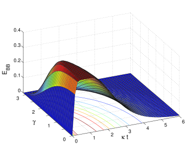
Figure 2: (Color online) Block-block entanglement as a function of the parameters $\kappa t$ and $\gamma$.

The genuine tripartite entanglement in the composite system can be quantified by the mixed state three-tangle won01pra

$$\tau_{3}(\rho_{ijk})=\mbox{min}\sum_{\{p_{x},\varphi^{(x)}_{ijk}\}}p_{x}\tau(\varphi_{ijk}^{(x)}),$$ (20)

where $\tau(\varphi^{(x)}_{ijk})=\tau_{i}-C_{ij}^{2}-C_{ik}^{2}$ ckw00pra is the pure state three-tangle and the minimum runs over all the pure state decompositions of $\rho_{ijk}$. The reduced density matrix of subsystem $c_{1}r_{1}c_{2}$ can be written as

$$\rho_{c_{1}r_{1}c_{2}}(t)=\varphi_{1}(t)+\varphi_{2}(t),$$ (21)

where the non-normalized pure state components are $|\varphi_{1}(t)\rangle=\alpha\mbox{cos}(\gamma/2)|000\rangle-\beta\mbox{sin}(\gamma/2)\xi|001\rangle+\alpha\mbox{sin}(\gamma/2)\chi|010\rangle+\alpha\mbox{sin}(\gamma/2)\xi|100\rangle+\beta\mbox{cos}(\gamma/2)\xi^{2}|101\rangle+\beta\mbox{cos}\xi\chi|011\rangle$ and $|\varphi_{2}(t)\rangle=\beta\mbox{sin}(\gamma/2)\chi|000\rangle-\beta\mbox{cos}(\gamma/2)\chi^{2}|010\rangle-\beta\mbox{cos}(\gamma/2)\xi\chi|100\rangle$, respectively. It is obvious that the $|\varphi_{2}\rangle$ is a separable state and its three-tangle is zero. Moreover, for the component $|\varphi_{1}\rangle$, we can derive $\tau(\varphi_{1})=0$. So, the decomposition in Eq. (21) is the optimal and the mixed state three-tangle $\tau_{3}(\rho_{c_{1}r_{1}c_{2}})$ is zero. Similarly, we can obtain that all the other mixed state three-tangles $\tau_{3}(\rho_{ijk})$ are zero.

Although all the $\tau_{3}(\rho_{ijk})$ are zero in the entanglement evolution, the three-qubit states are still entangled in the qubit-block form byw08pra ; loh06prl , which is not equivalent to the mixed state three-tangle and can not be accounted for the two-qubit entanglement. The qubit-block entanglement characterizes the genuine three-qubit entanglement under bipartite cut between a qubit and a block of qubits, and can be defined as $E_{q-B}(\rho_{i|jk})=C_{i|jk}^{2}-C_{ij}^{2}-C_{ik}^{2}$, in which the $C_{i|jk}$ quantifies bipartite entanglement between the qubits $i$ and $jk$. For the subsystems $c_{1}c_{2}r_{2}$ and $r_{1}c_{2}r_{2}$, their qubit-block entanglement are

$$E_{q-B}(\rho_{c_{1}|c_{2}r_{2}}) = C_{c_{1}|c_{2}r_{2}}^{2}-C_{c_{1}c_{2}}^{2}-C_{c_{1}r_{2}}^{2}$$

$$E_{q-B}(\rho_{r_{1}|c_{2}r_{2}}) = C_{r_{1}|c_{2}r_{2}}^{2}-C_{r_{1}r_{2}}^{2}-C_{c_{2}r_{1}}^{2},$$ (22)

where $C_{c_{1}|c_{2}r_{2}}^{2}=4\alpha^{2}\beta^{2}\xi^{2}$, $C_{r_{1}|c_{2}r_{2}}^{2}=4\alpha^{2}\beta^{2}\chi^{2}$, and the expressions of two-qubit concurrences $C_{ij}^{2}$ are given in Eqs. (12), (14) and (15).

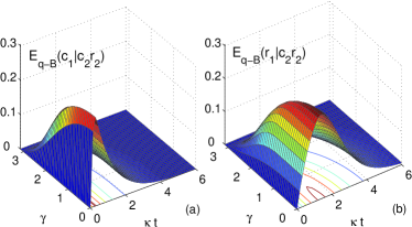
Figure 3: (Color online) (a) Qubit-block entanglement $E_{q-b}(c_{1}|c_{2}r_{2})$ and (b) qubit-block entanglement $E_{q-b}(r_{1}|c_{2}r_{2})$ as a function of the parameters $\kappa t$ and $\gamma$.

In Fig. 3, we plot the qubit-block entanglement as a function of the parameters $\kappa t$ and $\gamma$, where the initial state parameters are chosen as $\alpha=1/\sqrt{10}$ and $\beta=3/\sqrt{10}$. For a given value of the $\gamma$, the qubit-block entanglement $E_{c_{1}|c_{2}r_{2}}$ (in Fig. 3(a)) increases first with the time $\kappa t$, and then decreases with the $\kappa t$ after attaining to its maximal value. Along with the increase of the $\gamma$, the maximal value of $E_{c_{1}|c_{2}r_{2}}$ decreases. For the qubit-block entanglement $E_{r_{1}|c_{2}r_{2}}$ (in Fig. 3(b)), the trend of entanglement evolution is similar. In Refs. byw08pra ; byw09pra , it is pointed out that the qubit-block entanglement comes from the genuine multipartite entanglement in the enlarged pure state system. Here, for the multipartite cavity-reservoir system, we can derive the following relation

$$E_{BB}(\Psi_{t})=E_{q-B}(\rho_{c_{1}|c_{2}r_{2}}(t))+E_{q-B}(\rho_{r_{1}|c_{2}r_{2}}(t)),$$ (23)

which means that the qubit-block entanglement comes from the genuine block-block entanglement in the composite system.

V Entanglement transfer and entanglement transition under the LU operation

Because the evolution $U_{c_{1}r_{1}}(\hat{H},t)\otimes U_{c_{2}r_{2}}(\hat{H},t)$ are two local unitary operations under the partition $c_{1}r_{1}|c_{2}r_{2}$, the bipartite entanglement $C_{c_{1}r_{1}|c_{2}r_{2}}^{2}$ is invariant, and the following relation holds

$$C_{c_{1}r_{1}|c_{2}r_{2}}^{2}(\Psi_{t})=E_{BB}(t)+\sum C_{i^{\prime}j^{\prime}}^{2}(t)=4\alpha^{2}\beta^{2},$$ (24)

where $i^{\prime}\in\{c_{1},r_{1}\}$ and $j^{\prime}\in\{c_{2},r_{2}\}$, respectively. Therefore, in the multipartite cavity-reservoir system, we can characterize the entanglement evolution under a unified framework, where the two qubit entanglement transfer is quantified by the concurrence and the multipartite entanglement transition is quantified by the block-block entanglement $E_{BB}$. In Fig.4, the entanglement evolution modulated by different value of $\gamma$ is plotted, where $\gamma_{1}=2\mbox{arccos}(\sqrt{2/3})$, $\gamma_{2}=2\mbox{arccos}(\sqrt{1/3})$, and the initial state parameters are $\alpha=1/\sqrt{10}$ and $\beta=3/\sqrt{10}$.

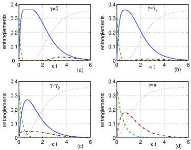
Figure 4: (Color online) Entanglement evolutions modulated by different parameter values: (a) $\gamma=0$, (b) $\gamma=\gamma_{1}$, (c) $\gamma=\gamma_{2}$ and (d) $\gamma=\pi$. The entanglements $C_{c_{1}c_{2}}^{2}$, $C_{r_{1}r_{2}}^{2}$, $C_{c_{1}r_{2}}^{2}+C_{c_{2}r_{1}}^{2}$ and $E_{BB}$ are represented by the green dashed line, red dotted line, brown dot-dashed line and blue solid line, respectively.

In Fig. 4(a), the parameter is chosen as $\gamma=0$, which corresponds to the symmetric initial state. In the time interval $\kappa t\in(0,\mbox{ln}(3/2))$, a part of the initial photon-photon entanglement $C_{c_{1}c_{2}}^{2}$ first transfers to the subsystems $c_{1}r_{2}$ and $c_{2}r_{1}$ (the brown dot-dashed line where a factor $5$ is multiplied), then the remaining photon-photon entanglement and the cavity-reservoir entanglement transition completely to the genuine block-block entanglement $E_{BB}$ (the blue solid line). Along with the time evolution, the block-block entanglement keeps invariant and is immune to the cavity-reservoir interaction in the time interval $\kappa t\in[\mbox{ln}(3/2),\mbox{ln}3]$. Finally, when $\kappa t\in(\mbox{ln}3,6]$, the multipartite entanglement $E_{BB}$ transitions to the two-qubit reservoir-reservoir entanglement (the red dotted line) and the cavity-reservoir entanglement. When the parameter $\gamma\in(0,\gamma_{1}]$, the trends of bipartite and multipartite entanglement evolutions are similar to those when $\gamma=0$, but the immune region of the block-block entanglement decreases with the parameter and the other evolution regions extend. In Fig. 4(b), the parameter is chosen as $\gamma=\gamma_{1}$, where the plateau region of the $E_{BB}$ changes to a point ($\kappa t=\mbox{ln}2$) and the procedures of entanglement transfer and entanglement transition need more time.

When the parameter $\gamma\in(\gamma_{1},\gamma_{2}]$, the initial photon entanglement transfers to not only the subsystems $c_{1}r_{2}$ and $c_{2}r_{1}$ but also the subsystem $r_{1}r_{2}$, and the two-qubit entanglement can not transition completely to the genuine block-block entanglement. As shown in Fig. 4(c), the entanglement transfer and entanglement transition are plotted when $\gamma=\gamma_{2}$. Along with the increase of the $\gamma$, the decay of the photon entanglement slows down and the transfer ratio of the two-qubit entanglement increases. At the same time, the transition ratio of the block-block entanglement decreases. In Fig. 4(d), the parameter is chosen as $\gamma=\pi$, in which the transition between the two-qubit entanglement and the multipartite entanglement disappears, and the entanglement evolution consists of only two-qubit entanglement transfer.

It should be pointed out that, in the unified framework of entanglement evolution, the entanglement monotone property of $E_{BB}$ is based on the numerical analysis on the average multipartite entanglement $E_{ms}$ byw07pra . The analytic proof is still an open problem.

VI Discussion and conclusion

In the more general case, an arbitrary initial state has the form $|\Psi_{0}^{g}\rangle=(\alpha_{1}|00\rangle+\alpha_{2}|01\rangle+\alpha_{3}|10\rangle+\alpha_{4}|11\rangle)_{c_{1}c_{2}}|00\rangle_{r_{1}r_{2}}$, which corresponds to two LU operations $U_{c_{1}}(\zeta_{1},\eta_{1},\gamma_{1},\delta_{1})\otimes U_{c_{2}}(\zeta_{2},\eta_{2},\gamma_{2},\delta_{2})$ acting on the symmetric initial state. In this case, the analytical characterization for the entanglement evolution is not available so far. However, the correlation between the ESD of cavity photons and the ESB of reservoirs still holds. This is because we can deduce the relation

$$\rho_{c_{1}c_{2}}^{g}(\xi,\chi)=S_{\xi\leftrightarrow\chi}[\rho_{r_{1}r_{2}}^{g}(\xi,\chi)],$$ (25)

where the evolution $U_{cr}(\hat{H},t)|10\rangle=\xi|10\rangle+\chi|01\rangle$ is used. Based on this relation, we can obtain that when the ESD of cavity photons occurs at the time $t_{ESD}=t_{0}$, the ESB of reservoirs will necessarily happen at the time $t_{ESB}=-(1/\kappa)\mbox{ln}[1-\mbox{exp}(-\kappa t_{0})]$. Moreover, the entanglement evolution is restricted by the monogamy relation

$$C_{c_{1}r_{1}|c_{2}r_{2}}^{2}(|\Psi_{0}^{g}\rangle) \geq C_{c_{1}c_{2}}^{2}(t)+C_{r_{1}r_{2}}^{2}(t)+C_{c_{1}r_{2}}^{2}(t),$$ (26)

$$+C_{c_{2}r_{1}}^{2}(t)$$

and the multipartite entanglement can be indicated by the two-qubit residual entanglement $M_{c_{1}r_{1}}$ byw09pra ; osb06prl .

The entanglement evolution with the asymmetric initial state is worth to consider for other physical systems, for example, the atoms systems tyu04prl , quantum dots and spin chains etc. dlo98pra ; ssl01pns ; xgw06pra . Moreover, the dissipative entanglement evolution has close relation with the type of the noise environment. Therefore, the non-Markovian environment, the correlated noises, and some operator channels bel07prl ; nov08pra ; kon08nat ; wan10epr are also worth to study in future.

In conclusion, we have investigated the entanglement evolution of multipartite cavity-reservoir systems with the asymmetric initial state. It is shown that there is only one parameter in the LU operation affecting the entanglement dynamics, which can delay the ESD of the photons, advance the ESB of the reservoirs, change the evolution route of bipartite entanglement, and suppress the multipartite entanglement. However, the correlation between the ESD and the ESB still holds. Furthermore, by defining the block-block entanglement, we analyze the multipartite entanglement evolution in the composite system, which allows us to study quantitatively both the entanglement transfer and the entanglement transition within a unified framework. Finally, the entanglement evolution with an arbitrary initial state is discussed.

Appendix

We first prove Eq. (5). The output state under the time evolution is

$$|\Phi_{t}\rangle = U_{c_{1}r_{1}}(\hat{H},t)\otimes U_{c_{2}r_{2}}(\hat{H},t)|\Phi_{0}^{a}\rangle$$ (27)

$$= U_{c_{1}}U_{c_{1}}^{\dagger}U_{c_{1}r_{1}}(\hat{H},t)\otimes U_{c_{2}r_{2}}(\hat{H},t)[U_{c_{1}}|\Phi_{0}\rangle],$$

where, in the second equation, the identity operator $I=U_{c_{1}}U_{c_{1}}^{\dagger}$ is inserted. Substituting the $U_{c_{1}}$ with the expression $R_{z}(\eta)R_{y}(\gamma)R_{z}(\delta)$ (we neglect the global phase $e^{i\zeta}$), we can obtain

$$|\Phi_{t}\rangle = U_{l}R_{z}^{\dagger}(\eta)U_{c_{1}r_{1}}(\hat{H},t)R_{z}(\eta)_{c_{1}}\otimes U_{c_{2}r_{2}}(\hat{H},t)$$

$$[R_{y}(\gamma)_{c_{1}}R_{z}(\delta)_{c_{1}}|\Phi_{0}\rangle]$$

$$\simeq U_{c_{1}r_{1}}(\hat{H}^{\prime},t)\otimes U_{c_{2}r_{2}}(\hat{H},t)[R_{y}(\gamma)_{c_{1}}R_{z}(\delta)_{c_{1}}|\Phi_{0}\rangle]$$

where the symbol $\simeq$ means the quantum states on the two sides are equivalent up to the local unitary operation $U_{l}=U_{c_{1}}R_{z}^{\dagger}(\delta)_{c_{1}}R_{y}^{\dagger}(\gamma)_{c_{1}}$ (note that entanglement is invariant under local unitary transformation), and we use the relation $R_{z}^{\dagger}(\eta)_{c_{1}}U_{c_{1}r_{1}}(\hat{H},t)R_{z}(\eta)_{c_{1}}=U_{c_{1}r_{1}}(\hat{H}^{\prime},t)$ with $\hat{H}^{\prime}=R_{z}^{\dagger}(\eta)_{c_{1}}\hat{H}R_{z}(\eta)_{c_{1}}$. Due to the symmetric property of initial state $|\Phi_{0}\rangle$, we have the relation $R_{z}(\delta)_{c_{1}}|\Phi_{0}\rangle=R_{z}(\delta)_{c_{2}}|\Phi_{0}\rangle$. Then the output state can be expressed further as

$$|\Phi_{t}\rangle = U_{c_{1}r_{1}}(\hat{H}^{\prime},t)\otimes R_{z}(\delta)_{c_{2}}R_{z}^{\dagger}(\delta)_{c_{2}}U_{c_{2}r_{2}}(\hat{H},t)R_{z}(\delta)_{c_{2}}$$ (29)

$$[R_{y}(\gamma)_{c_{1}}|\Phi_{0}\rangle]$$

$$\simeq U_{c_{1}r_{1}}(\hat{H}^{\prime},t)\otimes U_{c_{2}r_{2}}(\hat{H}^{\prime\prime},t)[R_{y}(\gamma)_{c_{1}}|\Phi_{0}\rangle],$$

where we insert the identity operator $R_{z}(\delta)_{c_{2}}R_{z}^{\dagger}(\delta)_{c_{2}}=I$ in the first equation and use the relation $\hat{H}^{\prime\prime}=R_{z}^{\dagger}(\delta)_{c_{2}}\hat{H}R_{z}(\delta)_{c_{2}}$ in the second equation.

Next, we will prove the effects of $\hat{H}^{\prime}$ and $\hat{H}^{\prime\prime}$ are equivalent to that of $\hat{H}$ in the entanglement evolution. Because the Hilbert space of subsystem $c_{1}r_{1}$ is spanned by $|00\rangle,|01\rangle,|10\rangle$, the creation and annihilation operators are

$$\hat{a}^{\dagger}=\left(\begin{array}[]{cc}0&0\\ 1&0\\ \end{array}\right)~{}\mbox{and}~{}\hat{a}=\left(\begin{array}[]{cc}0&1\\ 0&0\\ \end{array}\right),$$ (30)

respectively. With these expressions, the rotation operator $R_{z}(\eta)$ can be rewritten as

$$R_{z}(\eta)=A\cdot\hat{a}^{\dagger}\hat{a}+B,$$ (31)

where the coefficients $A=\mbox{exp}(i\eta/2)-\mbox{exp}(-i\eta/2)$ and $B=\mbox{exp}(-i\eta/2)$, respectively. After substituting the expression of $R_{z}(\eta)$ into the Hamiltonian $\hat{H}^{\prime}$, we can derive

$$\hat{H}^{\prime} = R_{z}^{\dagger}(\eta)_{c_{1}}\hat{H}R_{z}(\eta)_{c_{1}}$$ (32)

$$= (A\cdot\hat{a}^{\dagger}\hat{a}+B)^{\dagger}[\hbar\omega\hat{a}^{\dagger}\hat{a}+\hbar\sum_{k=1}^{N}\omega_{k}\hat{b}_{k}^{\dagger}\hat{b}_{k}$$

$$+\hbar\sum_{k=1}^{N}g_{k}(\hat{a}\hat{b}_{k}^{\dagger}+\hat{b}_{k}\hat{a}^{\dagger})](A\cdot\hat{a}^{\dagger}\hat{a}+B)$$

$$= \hbar\omega\hat{a}^{\dagger}\hat{a}+\hbar\sum_{k=1}^{N}\omega_{k}\hat{b}_{k}^{\dagger}\hat{b}_{k}+\hbar\sum_{k=1}^{N}g_{k}(\hat{a}\hat{b}_{k}^{\dagger}\cdot e^{i\eta}$$

$$+\hat{b}_{k}\hat{a}^{\dagger}\cdot e^{-i\eta})$$

$$= V_{r_{1}}^{\dagger}(\eta)\hat{H}V_{r_{1}}(\eta),$$

where $V_{r}(\eta)=\mbox{diag}\{1,\mbox{exp}(-i\eta)\}$, and we used the relations $\hat{a}^{\dagger}\hat{a}\hat{a}^{\dagger}\hat{a}=\hat{a}^{\dagger}\hat{a}=\hat{N}$ and $\hat{a}^{\dagger}\hat{N}\hat{b}_{k}=0$ expl1 . Similarly, for the Hamiltonian $\hat{H}^{\prime\prime}$, we can obtain

$$\hat{H}^{\prime\prime}=R_{z}^{\dagger}(\delta)_{c_{2}}\hat{H}R_{z}(\delta)_{c_{2}}=V_{r_{2}}^{\dagger}(\delta)\hat{H}V_{r_{2}}(\delta)$$ (33)

with $V_{r_{2}}(\delta)=\mbox{diag}\{1,\mbox{exp}(-i\delta)\}$. Therefore, the output state in Eq. (29) can be written as

$$|\Phi_{t}\rangle = V_{r_{1}}^{\dagger}(\eta)V_{r_{2}}^{\dagger}(\delta)U_{c_{1}r_{1}}(\hat{H},t)\otimes U_{c_{2}r_{2}}(\hat{H},t)$$ (34)

$$[R_{y}(\gamma)_{c_{1}}V_{r_{1}}(\eta)V_{r_{2}}(\delta)|\Phi_{0}\rangle].$$

In the above equation, the local unitary operation $V_{r_{1}}^{\dagger}(\eta)V_{r_{2}}^{\dagger}(\delta)$ does not change the entanglement evolution. Moreover, due to the reservoirs being in the vacuum state, we have $V_{r_{1}}(\eta)V_{r_{2}}(\delta)|\Phi_{0}\rangle=|\Phi_{0}\rangle$. Therefore, the effective output state in the entanglement evolution has the form

$$|\Psi_{t}\rangle=U_{c_{1}r_{1}}(\hat{H},t)\otimes U_{c_{2}r_{2}}(\hat{H},t)[R_{y}(\gamma)_{c_{1}}|\Phi_{0}\rangle].$$ (35)

This means that, for the asymmetric initial state modulated by an arbitrary LU operation $U_{c_{1}}(\zeta,\eta,\gamma,\delta)$, the entanglement evolution is only sensitive to the rotation $R_{y}(\gamma)$.

References

• (1) R. Horodecki P. Horodecki, M. Horodecki and K. Horodecki, Rev. Mod. Phys. 81, 865 (2009).
• (2) M. B. Plenio and S. Virmani, Quantum Inf. Comput. 7, 1 (2007).
• (3) Ting Yu and J. H. Eberly, Phys. Rev. Lett. 93, 140404 (2004); ibid. 97, 140403 (2006).
• (4) K. Życzkowski, P. Horodecki, M. Horodecki, and R. Horodecki, Phys. Rev. A 65, 012101 (2001).
• (5) A. K. Rajagopal and R. W. Rendell, Phys. Rev. A 63, 022116 (2001).
• (6) S. Daffer, K. Wodkiewicz, and J. K. Mclver, Phys. Rev. A 67, 062312 (2003).
• (7) P. J. Dodd and J. J. Halliwell, Phys. Rev. A 69, 052105 (2004).
• (8) M. Ban, J. Phys. A, 39, 1927 (2006).
• (9) M. F. Santos, P. Milman, L. Davidovich, and N. Zagury, Phys. Rev. A 73, 040305 (2006).
• (10) L. Derkacz and L. Jakóbczyk, Phys. Rev. A 74, 032313 (2006).
• (11) Z. Sun, X. Wang, and C. P. Sun, Phys. Rev. A 75, 062312 (2007).
• (12) Z.-G. Li, F.-S. Fei, Z. D. Wang and W.-M. Liu, Phys. Rev. A 79, 024303 (2009).
• (13) Z. Liu and H. Fan, Phys. Rev. A 79, 064305 (2009).
• (14) Q.-J. Tong, J.-H. An, H.-G. Luo, and C. H. Oh, Phys. Rev. A 81, 052330 2010.
• (15) Y. S. Weinstein, Phys. Rev. A 82, 032326 (2010).
• (16) T. Yu and J. H. Eberly, Science 323, 598 (2009).
• (17) M. P. Almeida, F. de Melo, M. Hor-Meyll, A. Salles, S. P. Walborn, P. H. Souto Ribeiro, L. Davidovich, Science 316, 579 (2007).
• (18) J. Laurat, K. S. Choi, H. Deng, C. W. Chou, and H. J. Kimble, Phys. Rev. Lett. 99, 180504 (2007).
• (19) C. E. López, G. Romero, F. Lastra, E. Solano, and J. C. Retamal, Phys. Rev. Lett. 101, 080503 (2008).
• (20) Y.-K. Bai, M.-Y. Ye, and Z. D. Wang, Phys. Rev. A 80, 044301 (2009).
• (21) M. A. Nielsen and I. L. Chuang, Quantum Computation and Quantum Information (Cambridge University Press, Cambridge, England, 2000), p20.
• (22) W. K. Wootters, Phys. Rev. Lett. 80, 2245 (1998).
• (23) The square root of the eigenvalues of matrix $R_{c_{1}c_{2}}$ are $\sqrt{\lambda_{1}}=\alpha\beta\xi^{2}+\sqrt{\beta^{2}\xi^{4}(\alpha^{2}+\beta^{2}cr^{4}\chi^{4})}$, $\sqrt{\lambda_{2}}=-\alpha\beta\xi^{2}+\sqrt{\beta^{2}\xi^{4}(\alpha^{2}+\beta^{2}cr^{4}\chi^{4})}$, and $\sqrt{\lambda_{3}}=\sqrt{\lambda_{4}}=\beta^{2}\xi^{2}\chi^{2}cr^{2}$ with $cr=\mbox{cos}(\gamma/2)$. The square root of the eigenvalues of matrix $R_{r_{1}r_{2}}$ are same to those of matrix $R_{c_{1}c_{2}}$ after exchanging the parameters $\xi$ and $\chi$.
• (24) A. R. R. Carvalho, F. Mintert, and A. Buchleitner, Phys. Rev. Lett. 93, 230501 (2004).
• (25) Y.-K. Bai, D. Yang, and Z. D. Wang, Phys. Rev. A 76, 022336 (2007).
• (26) Y.-K. Bai and Z. D. Wang, Phys. Rev. A 77, 032313 (2008).
• (27) X.-J. Ren, W. Jiang, X. Zhou, Z. W. Zhou, and G. C. Guo, Phys. Rev. A 78, 012343 (2008).
• (28) A. Wong and N. Christensen, Phys. Rev. A 63, 044301 (2001).
• (29) V. Coffman, J. Kundu, and W. K. Wootters, Phys. Rev. A 61, 052306 (2000).
• (30) R. Lohmayer, A. Osterloh, J. Siewert, and A. Uhlmann, Phys. Rev. Lett. 97, 260502 (2006).
• (31) Y.-K. Bai, M.-Y. Ye, and Z. D. Wang, Phys. Rev. A 78, 062325 (2008).
• (32) T. J. Osborne and F. Verstraete, Phys. Rev. Lett. 96, 220503 (2006).
• (33) D. Loss and D. V. DiVincenzo, Phys. Rev. A 57, 120 (1998).
• (34) S.-S. Li, G.-L. Long, F.-S. Bai, S.-L. Feng, and H.-Z. Zheng, Proc. Natl. Acad. Sci. U.S.A. 98, 11847 (2001).
• (35) X. Wang and Z. D. Wang, Phys. Rev. A 73, 064302 (2006).
• (36) B. Bellomo, R. Lo Franco, and G. Compagno, Phys. Rev. Lett. 99, 160502 (2007).
• (37) E. Novais, E. R. Mucciolo, and H. U. Baranger, Phys. Rev. A 78, 012314 (2008).
• (38) T. Konrad, F. De Melo, M Tiersch, C. Kasztelan, A. Aragao, and A. Buchleitner, Nature Physics 4, 99 (2008).
• (39) X.-B. Wang, Z.-W. Yu and J.-Z. Hu, arXiv:1001.0156.
• (40) Due to the space of system $c_{1}r_{1}$ is spanned by $\{|00\rangle,|01\rangle,|10\rangle\}$, we have $(\hat{a}^{\dagger}\hat{a}-1)\hat{a}^{\dagger}\hat{a}=0\Rightarrow\hat{N}^{2}=\hat{N}$. Similarly, according to the space of system $c_{1}r_{1}$, we have $\hat{a}^{\dagger}\hat{b}\hat{b}^{\dagger}\hat{b}\hat{N}=0$. Combining it with the commutation relation of $\hat{b}$ and $\hat{b}^{\dagger}$, we can derive $\hat{a}^{\dagger}\hat{N}\hat{b}_{k}=0$.