A master solution of the quantum Yang-Baxter equation
and classical discrete integrable equations

Abstract

We obtain a new solution of the star-triangle relation with positive Boltzmann weights which contains as special cases all continuous and discrete spin solutions of this relation, that were previously known. This new master solution defines an exactly solvable 2D lattice model of statistical mechanics, which involves continuous spin variables, living on a circle, and contains two temperature-like parameters. If one of the these parameters approaches a root of unity (corresponds to zero temperature), the spin variables freezes into discrete positions, equidistantly spaced on the circle. An absolute orientation of these positions on the circle slowly changes between lattice sites by overall rotations. Allowed configurations of these rotations are described by classical discrete integrable equations, closely related to the famous $Q_{4}$-equations by Adler Bobenko and Suris. Fluctuations between degenerate ground states in the vicinity of zero temperature are described by a rather general integrable lattice model with discrete spin variables. In some simple special cases the latter reduces to the Kashiwara-Miwa and chiral Potts models.

Department of Theoretical Physics,
Research School of Physics and Engineering,
Australian National University, Canberra, ACT 0200, Australia.
E-mail: Vladimir.Bazhanov@anu.edu.au

Faculty of Information Sciences and Engineering,
University of Canberra, Bruce ACT 2601, Australia.
E-mail: Sergey.Sergeev@canberra.edu.au

1 Introduction

There are only a few exactly solvable models in statistical mechanincs where the Yang-Baxter equation takes its distinguished “star-triangular” form. The most notable discrete-spin models in this class are the Kashwara-Miwa [1] and chiral Potts [2, 3, 4] models (both of them also contain the Ising model [5] and Fateev-Zamolodchikov $Z_{N}$-model [6] as particular cases) see [7] for a review. There are also important continuous spin models, including Zamolodchikov’s “fishing-net” model [8], which describes certain planar Feynman diagrams in quantum field theory, and the Faddeev-Volkov model [9], connected with quantization [10] of discrete conformal transformations [11, 12]. All above models are also distiguished by the positivity of the Boltzmann weights — the property that is required for many applications, but rarely realized for generic solutions of the Yang-Baxter equation.

In this paper we present new solutions of the star-triangle relation which possess the positivity property. Most importantly we present a master solution, which contains as special cases all the previously known continuous and discrete spin solutions mentioned above, and also leads to new ones. Our master solution involves continouos real-valued spins, varying in the range  $0\leq x,y<2\pi$,  and a reflection-symmetric Boltzmann weight, which is unchanged upon interchanging the spins $x,y$,

$${\mathcal{W}}_{\alpha}(x,y)={\mathcal{W}}_{\alpha}(y,x)\;=\;\kappa_{\alpha}^{-1}\;\frac{\Phi(x-y+\mathsf{i}\alpha)}{\Phi(x-y-\mathsf{i}\alpha)}\;\frac{\Phi(x+y+\mathsf{i}\alpha)}{\Phi(x+y-\mathsf{i}\alpha)}\;,$$ (1.1)

and depends on an additive spectral parameter $\alpha$ (it enters additively into the Yang-Baxter equation (1.5) below). Here $\kappa_{\alpha}$ is a spin-independent normalization factor and $\Phi(s)$ is the elliptic $\Gamma$-function [13, 14, 15] ,

$$\Phi(s)\;=\;\exp\left\{\sum_{n\neq 0}\frac{\textrm{{\large e}}^{-\mathsf{i}ns}}{n\,({\mathsf{p}}^{n}-{\mathsf{p}}^{-n})\,({\mathsf{q}}^{n}-{\mathsf{q}}^{-n})}\right\}\;.$$ (1.2)

The latter depends on two fixed parameters ${\mathsf{p}}$ and ${\mathsf{q}}$ (elliptic nomes),

$${\mathsf{p}}\;=\;\textrm{{\large e}}^{\mathsf{i}\pi\tau}\;,\quad{\mathsf{q}}=\textrm{{\large e}}^{\mathsf{i}\pi\sigma}\;,\quad{\eta}\;=\;-\mathsf{i}\pi\,(\tau+\sigma)\;,\quad\mathop{\hbox{\rm Im}}\nolimits\tau>0,\quad\mathop{\hbox{\rm Im}}\nolimits\sigma>0\ .$$ (1.3)

This function obeys a simple functional equation $\Phi(s)\,\Phi(-s)\equiv 1$, which ensures the reflection symmetry of the weight (1.1). Define also a single-spin weight

$${\mathcal{S}}(x)\;=\;\frac{\textrm{{\large e}}^{{\eta}/{4}}}{4\pi}\,\vartheta_{1}(x\,|\,\tau)\,\vartheta_{1}(x\,|\,\sigma)\;,$$ (1.4)

where $\vartheta_{j}(z\,|\,\tau)$,  $j=1,2,3,4$,  are the standard Jacobi theta-functions [16] with the periods $\pi$ and $\pi\tau$.

We state that the above weights satisfy the star-triangle relation of the form,

$$\begin{array}[]{l}\displaystyle\int_{0}^{2\pi}\ dx_{0}\ {\mathcal{S}}(x_{0})\ {{\mathcal{W}}}_{{\eta}-\alpha_{1}}(x_{1},x_{0})\ {{\mathcal{W}}}_{\alpha_{1}+\alpha_{3}}(x_{2},x_{0})\ {\mathcal{W}}_{{\eta}-\alpha_{3}}(x_{3},x_{0})\\[11.38092pt] \phantom{\displaystyle\sum_{\sigma}S(\sigma){W}({\eta}-\theta_{1}\,|\,a,\sigma)\,{W}({\eta}-{\eta}{\eta})}={\cal R}\ {\mathcal{W}}_{\alpha_{1}}(x_{2},x_{3})\ {\mathcal{W}}_{{\eta}-\alpha_{1}-\alpha_{3}}(x_{1},x_{3})\ {\mathcal{W}}_{\alpha_{3}}(x_{1},x_{2}),\end{array}$$ (1.5)

where the crossing parameter ${\eta}$ is defined in (1.3) and ${\cal R}$ is some explicitly known scalar factor (see (2.36) below) which depends on the spectral variables $\alpha_{1}$ and $\alpha_{3}$, but is independent of the spins $x_{1},x_{2},x_{3}$.

The weights (1.1) and (1.4) are real and positive in (at least) two main physical regimes

$$\mbox{(i)}\quad{\mathsf{p}}={\mathsf{p}}^{*},\quad{\mathsf{q}}={\mathsf{q}}^{*}\qquad\qquad\mbox{or}\qquad\mbox{(ii)}\quad{\mathsf{p}}={\mathsf{q}}^{*}\ ,$$ (1.6)

with real spins and a real spectral parameter in the range $0<\alpha<{\eta}$. Note, also that the weights are unchanged upon negating the spins ${\mathcal{W}}_{\alpha}(x,y)={\mathcal{W}}_{\alpha}(\pm x,y)={\mathcal{W}}_{\alpha}(x,\pm y)$,  ${\mathcal{S}}(x)={\mathcal{S}}(-x)$,  and are periodic in each spin argument

$${\mathcal{W}}_{\alpha}(x,y)={\mathcal{W}}_{\alpha}(x+2\pi,y)={\mathcal{W}}_{\alpha}(x,y+2\pi),\qquad{\mathcal{S}}(x)={\mathcal{S}}(x+2\pi),$$ (1.7)

therefore one can regard the spins as angle variables on a circle. This also means that the integral in (1.5) is a closed contour integral, where the integration contour can be deformed into the complex plane, if necessary.

As is well known [17] every solution of the star-triangle relation can be used to define exactly solvable edge interaction models on various two-dimensional lattices. For purposes of this introduction it is enough to consider an homogeneous square lattice. In this case the partition function reads

$${\cal Z}=\mathop{\idotsint}_{0\leq x_{m}<2\pi\phantom{|}}\ \prod_{(ij)}{\mathcal{W}}_{\alpha}(x_{i},x_{j})\ \prod_{(kl)}{\mathcal{W}}_{{\eta}-\alpha}(x_{k},x_{l})\ \prod_{m}{\mathcal{S}}(x_{m})\,dx_{m}$$ (1.8)

where the first product is taken over all horizontal edges $(ij)$, the second over all vertical edges $(kl)$ and the third over all internal sites $m$ of the lattice. We will implicitly assume fixed boundary conditions. In the limit of a large lattice the partition function can be calculated with the inversion relation method [18, 19, 20]; the result is given in (2.44).

The elliptic $\Gamma$-function (1.2) first appeared implicitly in Baxter’s pioneering paper [21] on the 8-vertex (it enters the exact expression for the partition function) and then was developed systematically in [13, 14, 15]. Our key observation is that as a mathematical identity the star-triangle relation (1.5) reduces to the most general form of Spiridonov’s celebrated elliptic beta integral [15]. Actually, it is quite remarkable that this fundamental integral identity, which lies at the basis of the theory of elliptic hypergeometric functions [22], is nothing but a Yang-Baxter (star-triangle) relation, defining a perfectly physical integrable lattice model of statistical mechanics.

Let us now explain how this continuous-spin model could turn into a model with discrete spin variables, for instance, into the chiral Potts model. The key to the answer is the low-temperature limit. Note that the weights (1.1) and (1.4) symmetrically depend on two temperature-like parameter ${\mathsf{p}}$ and ${\mathsf{q}}$. For generic values of these parameters,  $0<|{\mathsf{p}}|,|{\mathsf{q}}|<1$,   the formula (1.1) defines a smooth function of spins with two dull bell-shaped maxima near $x=y$ and $x=2\pi-y$. However, when one of the parameters $p,q$ approaches the unit circle, the maxima become very sharp. Moreover, the function (1.1) starts to exhibit additional sharp ($\delta$-function type) maxima, so that the spin variables become locked to a discrete set of energetically favourable positions. To get a better idea of how this happens, consider the limit when ${\mathsf{q}}$ approaches a root of unity

$${\mathsf{p}}=\textrm{{\large e}}^{i\pi\tau}=\mbox{fixed},\qquad{\mathsf{q}}=\textrm{{\large e}}^{-\rho\,T}\textrm{{\large e}}^{\mathsf{i}\pi/N}\;,\qquad T\to 0,\qquad N\geq 1\ ,$$ (1.9)

and $\rho$ is some suitable chosen numerical coefficient. The partition function (1.8) develops a typical low-temperature asymptotics

$${\cal Z}=\mathop{\idotsint}_{0\leq x_{m}<2\pi\phantom{|}}\ \ \exp\Big{(}-\frac{{\cal E}\big{(}X\big{)}}{T}+O(1)+O(T)\Big{)}\ \prod_{m}\frac{dx_{m}}{\sqrt{T}}\ ,\qquad T\to 0\ ,$$ (1.10)

where $X=\{x_{1},x_{2},\ldots,x_{M}\}$ and $M$ is the number of internal (non-boundary) sites of the lattice. Explicit expressions for the energy functional ${\cal E}\big{(}X\big{)}$ are given in Section 3.3 and Appendix Acknowledgements. It is a bounded from below function of the spin variables and that for $N>1$ it has stronger periodicity properties in each spin variable

$${\cal E}\big{(}x_{1},x_{2},\ldots,x_{m}+{\textstyle\frac{2\pi}{N}}\,,\ldots,x_{M}\big{)}={\cal E}\big{(}x_{1},x_{2},\ldots,x_{m}\,,\ldots,x_{M}\big{)},\quad m=1,\ldots,M\ ,$$ (1.11)

than could be expected from (1.7). To obtain the leading asymptotics of the partition function (1.10) at $T\to 0$, one has to minimize ${\cal E}\big{(}X\big{)}$,

$$\log{\cal Z}=-\frac{{\mathcal{E}}(X^{(cl)})}{T}+\log{\cal Z}_{0}+O(T),$$ (1.12)

where

$$\frac{{\partial{\mathcal{E}}}\big{(}X\big{)}}{\partial x_{m}}\Big{|}_{X=X^{(cl)}}=0,\qquad m=1,2,\ldots,M\ ,$$ (1.13)

and $X^{(cl)}=\{\xi_{1},\xi_{2},\ldots,\xi_{M}\}$  denotes an stationary point of the functional ${\mathcal{E}}(X)$, corresponding to the ground state of the system. Remembering that the spin variables run over the full circle $0\leq x_{m}<2\pi$, one immediately concludes that this ground state is $N^{M}$- fold degenerate. Indeed, thanks to (1.11), the equilibrium positions can be independently shifted,

$$\xi_{m}\to\xi_{m}+{2\pi n_{m}}/{N},\qquad n_{m}\in{\mathbb{Z}}_{N}\equiv\{0,1,\ldots,N-1\},$$ (1.14)

without affecting the validity of the conditions (1.13). Thus at zero temperature, $T=0$, the system “freezes” into one of these degenerate ground state configurations.

The next natural question is to understand what is happening in the vicinity of the zero temperature, when the above degeneracy is lifted. A simple analysis shows that the only fluctuations, that are allowed in the next-to-leading order of the low-temperature expansion, are the discrete flips (1.14) between different ground state configurations, whereas the values of $\xi_{m}\pmod{2\pi/N}$ arising from the minimisation of  ${\cal E}(X)$ remain frozen. This means that the quantity ${\cal Z}_{0}$ in constant term of the expansion (1.12) can be understood as the partition function of a certain edge interaction model with discrete spins variable $\{n_{1},n_{2},\ldots,n_{M}\}$, each taking $N$ different values $n_{k}\in{\mathbb{Z}}_{N}$. Its Boltzmann weights can be found by expanding (1.8) in the limit (1.9) and isolating all constant terms. The results are given in Section 4. Naturally, these Boltzmann weights explicitly depend on the original additive spectral variables $\alpha$ and ${\eta}-\alpha$, and the remaining temperature-like parameter ${\mathsf{p}}$ (which is still at our disposal). Moreover, they also depend on the variables $\{\xi_{m}\}$, which solves the minimization equation (1.13), and this is what makes the problem really complicated. In particular, the variables $\{\xi_{m}\}$  could depend on the original spectral variables $\alpha$ and ${\eta}-\alpha$ in a very complicated way, therefore, in general, the simple addition law for the spectral parameters in the star-triangle relation will be lost. Nevertheless, we definitely know that the emerging discrete spin model must be integrable! Indeed the original master model is integrable for any value of parameter ${\mathsf{q}}$, therefore this integrability should manifests itself in every order of the expansion (1.12).

It is clear, of course, that to analytically describe the new discrete spin model one needs to better understand the minimisation equations (1.13), which according to our expectations must be integrable as well. The energy functional ${\cal E}(X)$ is a sum of two-spin edge energies therefore the variational equation (1.13) for any particular spin $x_{m}$ will also involve spins on all neighbouring sites. For the square lattice each site has four (nearest) neighbours, therefore each equation (1.13) will contain five variables. For the homogeneous model (1.8) on the square lattice they have the same form for any internal spin $\xi$,

$$\widetilde{\Psi}_{3}\big{(}\xi,\xi_{r}\big{)}\widetilde{\Psi}_{3}(\xi,\xi_{\ell})=\widetilde{\Psi}_{1}\big{(}\xi,\xi_{u}\big{)}\widetilde{\Psi}_{1}(\xi,\xi_{d})\ ,$$ (1.15)

where $\xi_{u},\xi_{d},\xi_{\ell},\xi_{r}$ are the spins immediately above, below, to the left and to the right of $\xi$. The function $\widetilde{\Psi}_{j}(x,y)$ reads

$$\widetilde{\Psi}_{j}(x,y)\;=\;\frac{\vartheta_{j}\big{(}\frac{N}{2}(x-y+\mathsf{i}\alpha)\,|\,N\tau\big{)}_{\phantom{|}}\vartheta_{j}\big{(}\frac{N}{2}(x+y+\mathsf{i}\alpha)\,|\,N\tau\big{)}}{\vartheta_{j}\big{(}\frac{N}{2}(x-y-\mathsf{i}\alpha)\,|\,N\tau\big{)}^{\phantom{|}}\vartheta_{j}\big{(}\frac{N}{2}(x+y-\mathsf{i}\alpha\,)|\,N\tau\big{)}}\ ,\qquad j=1,2,3,4.$$ (1.16)

Our next important observation is that these non-linear difference equations are indeed integrable, as expected. They appeared previously in remarkable papers by Adler, Bobenko and Suris [24, 25] devoted to the classification of classical integrable equations on planar quadrilateral graphs. More specifically, the minimization equation (1.13) arising here is closely related with the so-called $Q_{4}$ equation, which is the most complicated equation located at the top of the Adler-Bobenko-Suris classification.

The organization of the paper is as follows. In Section 2 we briefly review some basic facts from the theory of integrable lattice models and present the master solution (1.1), (1.4). The low-temperature expansion is considered in Section 3. In Section 4 we present a new discrete spin solution of the star-triangle relation and show that in some simple special cases this solution reduces to those of the Kashiwara-Miwa [1] and chiral Potts [2, 3, 4] models (the latter were the most complicated solvable discrete spin models hitherto known). Here we present only final results; the details of calculations will be published separately.

2 The star-triangle relation

2.1 Edge interaction models

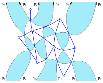
Figure 1: The planar graph $\mathscr{G}$ (shown by open circles and bold edges) and its medial graph ${\mathscr{L}}$ (shown by thin edges and alternatively shaded faces).

To facilitate further discussions let us briefly review some basic facts from the theory of integrable lattice models. A general solvable edge-interaction model on a planar graph can be defined in the following way [26, 27]. Consider a planar graph ${\mathscr{G}}$, of the type shown in Fig.1, where its sites (or vertices) are drawn by open circles and the edges by bold lines. The same figure also contains another graph ${\mathscr{L}}$, shown by thin lines, which is the medial graph for ${\mathscr{G}}$. The faces of ${{\mathscr{L}}}$ are shaded alternatively; the sites of ${\mathscr{G}}$ are placed on the unshaded faces. We assume that for each line of ${\mathscr{L}}$ one can assign a direction, so that all the lines head generally from the bottom of the graph to the top. They can go locally downwards, but there can be no closed directed paths in $\mathscr{L}$. This means that one can always distort $\mathscr{L}$, without changing its topology, so that the lines always head upwards.

Now we define a statistical mechanical model on $\mathscr{G}$. With each line $\ell$ of ${\mathscr{L}}$ associate its own “rapidity” variable $p_{\ell}$. At each site $i$ of $\mathscr{G}$  place a spin $s_{i}$, taking some set of (continuous or discrete) values. Two spins interact only if they are connected by an edge. This means that each edge is assigned with a Boltzmann weight which depends on spins at the ends of the edge. The Boltzmann weights usually depend on some global parameters of the model which are same for all edges (for instance, temperature-like variables). Here we assume that they also depend on local parameters, namely, on the two rapidity variables associated with the edge.

Figure 2: Edges of the first (left) and second types and their Boltzmann weights.

The edges of $\mathscr{G}$ are either of the first type in Fig. 2, or the second. Let $a$, $b$ be the spins at the end sites of the edge and $p$, $q$ the rapidities of the associated lines, arranged as in Fig. 2. Then if the edge is of the first type, the spins $a$, $b$ interact with the Boltzmann weight function $W_{pq}(a,b)$. If the edge is of the second type, they interact with the weight $\overline{W}_{pq}(a,b)$. In general, there may also be a single-spin self-interaction with a rapidity-independent weight $S(a)$ for each spin $a$. The partition function is defined as

$$Z=\sum_{\{s\}}\ \prod_{(ij)}W_{pq}(s_{i},s_{j})\ \prod_{(kl)}\overline{W}_{pq}(s_{k},s_{l})\ \prod_{m}S(s_{m})$$ (2.17)

where the first product is over all edges $(ij)$ of the first type, the second is over all edges $(kl)$ of the second type, and the third one is over all sites $m$. The sum is taken over the values of spins on the internal sites, while the boundary spins are kept fixed (for continuous spins the sum is replaced by an integral). The integrability requires the weights to satisfy the two star-triangle relation [7]

$$\sum_{d}S(d)\,\overline{W}_{pq}(d,c)W_{pr}(b,d)\overline{W}_{qr}(a,d) \!\!=\!\! {R}_{pqr}\,W_{pq}(b,a)\overline{W}_{pr}(a,c)W_{qr}(b,c)$$

$$\sum_{d}S(d)\,\overline{W}_{pq}(c,d)W_{pr}(d,b)\overline{W}_{qr}(d,a) \!\!=\!\! {R}_{pqr}\,W_{pq}(a,b)\overline{W}_{pr}(c,a)W_{qr}(c,b)$$

where ${R}_{pqr}$ is some factor independent of the spins $a,b,c$. For all known solutions it can be written in the form [28, 7],

$$R_{pqr}=f_{qr}f_{pq}/f_{pr},$$ (2.19)

where $f_{pq}$ is a scalar function of the two rapidity variables $p$ and $q$. Moreover, the weights can always be normalized so that they satisfy the two inversion relations,

$$\begin{array}[]{rcl}\displaystyle\,\sum_{c}\overline{W}_{pq}(a,c)\,S(c)\,\overline{W}_{qp}(c,b)&=&S(a)^{-1}\,f_{pq}\,f_{qp}\,\delta_{ab}\ ,\\[8.5359pt] W_{pq}(a,b)\,W_{qp}(a,b)&=&1,\qquad\forall a,b\ .\end{array}$$ (2.22)

The first star-triangle relation in (LABEL:str-bax) equates partition functions of the “star” and “triangle” graphs shown in Fig. 3, where the external spins $a$, $b$ and $c$ are being fixed. Similarly, the second relation in (LABEL:str-bax) is related to a mirror image of Fig. 3.

Figure 3: A pictorial representation of the first star-triangle relation in (LABEL:str-bax).

Note that the two relations coincide for reflection-symmetric models,

$$W_{pq}(a,b)=W_{pq}(b,a),\qquad\overline{W}_{pq}(a,b)=\overline{W}_{pq}(b,a),$$ (2.23)

where the weights are unchanged by interchanging the spins $a$ and $b$.

The partition function (2.17) possesses remarkable invariance properties [26, 27]. It remains unchanged by continuously deforming the lines of ${\mathscr{L}}$ with their boundary positions kept fixed, as long as the graph ${\mathscr{L}}$ remains directed. It is easy to see that all such transformations reduce to a combination of the moves, corresponding to the star-triangle (LABEL:str-bax) and inversion relations (2.22). In general the partition function acquire simple $f_{pq}$ factors under these moves, however with an appropriate normalization of the Boltzmann weights the invariance is strict (all extra factors could be eliminated, see (2.38)). Given that the graphs ${\mathscr{L}}$ and ${\mathscr{G}}$ can undergo rather drastic changes, the above invariance, called “$Z$-invariance” in [26], is rather non-trivial. It provides an ultimate formulation of the integrability statement. For instance, the commutativity of transfer matrices in solvable models is a particular case of this invariance.

2.2 The master solution of the star-triangle relation

The star-triangle relation (1.5) is a particular case of (LABEL:str-bax), where the Boltzmann weights are reflection-symmetric and possess the difference property, which means that they depend only a difference of two rapidities $p$ and $q$,

$$W_{pq}(a,b)\to{\cal W}_{p-q}(a,b),\qquad\overline{W}_{pq}(a,b)\to{\cal W}_{{\eta}-p+q}(a,b).$$ (2.24)

With this correspondence the spectral variables $\alpha_{1}$ and $\alpha_{3}$ in (1.5) are connected to the rapidity variables in (LABEL:str-bax) as

$$\alpha_{1}=q-r,\qquad\alpha_{3}=p-q\ .$$ (2.25)

Note also that the fact that the weights for the edges of two types in Fig. 2 are obtained from each other by a simple substitution $\alpha\to{\eta}-\alpha$   of the difference variable $\alpha=p-q$ is called the crossing symmetry. By this reason the parameter ${\eta}$ in (2.24) is usually called the “crossing parameter”.

The standard elliptic $\Gamma$-function is defined as (see, e.g., Eq.(2.18) of [22]),

$$\Gamma(z;{\mathsf{p}}^{2},{\mathsf{q}}^{2})\;\stackrel{{\scriptstyle\textrm{def}}}{{=}}\;\prod_{n,m=0}^{\infty}\frac{1-z^{-1}{\mathsf{p}}^{2n+2}\,{\mathsf{q}}^{2m+2}}{1-z\,{\mathsf{p}}^{2n}\,{\mathsf{q}}^{2m}}\;,$$ (2.26)

where

$${\mathsf{p}}\;=\;\textrm{{\large e}}^{\mathsf{i}\pi\tau}\;,\quad{\mathsf{q}}=\textrm{{\large e}}^{\mathsf{i}\pi\sigma}\;,$$ (2.27)

and $0<|{\mathsf{p}}|,|{\mathsf{q}}|<1$. Define the crossing parameter ${\eta}$ by

$$\textrm{{\large e}}^{-\eta}\;=\;{\mathsf{p}}{\mathsf{q}}\;,\quad\eta\;=\;-\mathsf{i}{\pi}(\tau+\sigma)\;.$$ (2.28)

For our purposes it is convenient to use the function

$$\Phi(x)\;\stackrel{{\scriptstyle\textrm{def}}}{{=}}\;\Gamma(\textrm{{\large e}}^{-\mathsf{i}(x-\mathsf{i}\eta)};{\mathsf{p}}^{2},{\mathsf{q}}^{2})\;=\;\exp\left\{\sum_{n\neq 0}\frac{\textrm{{\large e}}^{-\mathsf{i}xn}}{n({\mathsf{p}}^{n}-{\mathsf{p}}^{-n})({\mathsf{q}}^{n}-{\mathsf{q}}^{-n})}\right\}\;,$$ (2.29)

which satisfies a simple “reflection” equation $\Phi(x)\Phi(-x)=1$.

Our master solution of the star-triangle equation (1.5) (already quoted in the introduction) reads

$${\mathcal{W}}_{\alpha}(x,y) = \kappa(\alpha)^{-1}\,\frac{\Phi(x-y+\mathsf{i}\alpha)}{\Phi(x-y-\mathsf{i}\alpha)}\;\frac{\Phi(x+y+\mathsf{i}\alpha)}{\Phi(x+y-\mathsf{i}\alpha)}\;,$$ (2.30)

$${\mathcal{S}}(x) = \frac{\textrm{{\large e}}^{\eta/4}}{4\pi}\vartheta_{1}(x\,|\,\tau)\vartheta_{1}(x\,|\,\sigma)\;.$$ (2.31)

where $\vartheta_{j}(z\,|\,\tau)$,  $j=1,2,3,4$,  are the standard Jacobi theta-functions [16] with the periods $\pi$ and $\pi\tau$. The weights are symmetric,

$${\mathcal{W}}_{\alpha}(x,y)={\mathcal{W}}_{\alpha}(y,x)={\mathcal{W}}_{\alpha}(\pm x,y)={\mathcal{W}}_{\alpha}(x,\pm y)\,,\qquad{\mathcal{S}}(x)={\mathcal{S}}(-x),$$ (2.32)

periodic in their spin arguments,

$${\mathcal{W}}_{\alpha}(x,y)={\mathcal{W}}_{\alpha}(x+2\pi,y)={\mathcal{W}}_{\alpha}(x,y+2\pi),\qquad{\mathcal{S}}(x)={\mathcal{S}}(x+2\pi),$$ (2.33)

and satisfy the recurrence relations

$$\frac{{\mathcal{W}}_{\alpha}\big{(}x-{\pi\sigma},y\big{)}_{\phantom{|}}}{{\mathcal{W}}_{\alpha}\big{(}x+\pi\sigma,y\big{)}^{\phantom{|}}}\;=\;\frac{\vartheta_{4}\big{(}\frac{1}{2}(x-y+\mathsf{i}\alpha)\,|\,\tau\big{)}_{\phantom{|}}}{\vartheta_{4}\big{(}\frac{1}{2}(x-y-\mathsf{i}\alpha)\,|\,\tau\big{)}^{\phantom{|}}}\frac{\vartheta_{4}\big{(}\frac{1}{2}(x+y+\mathsf{i}\alpha)\,|\,\tau\big{)}_{\phantom{|}}}{\vartheta_{4}\big{(}\frac{1}{2}(x+y-\mathsf{i}\alpha)\,|\,\tau\big{)}^{\phantom{|}}}\;,\quad\textrm{and the same with}\ \tau\leftrightarrow\sigma\;.$$ (2.34)

For real-valued spins the weights are real and positive in the two main physical regimes

$$\mbox{(i)}\quad{\mathsf{p}}={\mathsf{p}}^{*},\quad{\mathsf{q}}={\mathsf{q}}^{*}\qquad\qquad\mbox{or}\qquad\mbox{(ii)}\quad{\mathsf{p}}={\mathsf{q}}^{*}\ ,$$ (2.35)

provided the spectral parameter is real and kept in the range $0<\alpha<{\eta}$.

As a mathematical identity the star-triangle relation (1.5) contains seven continuous parameters: two nomes ${\mathsf{p}}$ and ${\mathsf{q}}$; two spectral variables $\alpha_{1}$ and $\alpha_{3}$; and three spins $x_{1},x_{2},x_{3}$. One can show that this relation can be reduced to the most general form of Spiridonov’s celebrated elliptic beta integral. Then using Eq.(3.1) of [22] one obtains the expression for the factor ${\cal R}$ in (1.5),

$${\cal R}=\frac{f(\alpha_{1})\,f(\alpha_{3})}{f({\alpha_{1}+\alpha_{3}})},\qquad{f(\alpha)}=\Phi(\mathsf{i}{\eta}-2\mathsf{i}\alpha)\,\frac{\kappa(\alpha)}{\kappa({\eta}-\alpha)}\ ,$$ (2.36)

It is worth noting that if the function $\kappa(\alpha)$ satisfies the equations

$$\frac{\kappa(\eta-\alpha)}{\kappa(\alpha)}\;=\;\Phi(\mathsf{i}{\eta}-2\mathsf{i}\alpha)\;,\quad\kappa(\alpha)\kappa(-\alpha)=1\;,$$ (2.37)

then one trivially obtains

$$f(\alpha)\equiv 1,\qquad{\cal R}\equiv 1\ .$$ (2.38)

With this normalization the inversion relations (2.22) for the weights (2.30) and (2.31) simplify to

$$\int_{0}^{2\pi}dz\,{\mathcal{S}}(z)\,{\mathcal{W}}_{\eta-\alpha}(x,z)\,{\mathcal{W}}_{\eta+\alpha}(z,y) = \frac{1}{2{\mathcal{S}}(x)}\left(\delta(x-y)+\delta(x+y)\right)\;,$$

$${\mathcal{W}}_{\alpha}(x,y)\,{\mathcal{W}}_{-\alpha}(x,y) = 1\,,$$

where $\delta(x)$ denotes the periodic $\delta$-function

$$\delta(x)=\frac{1}{2\pi}\sum_{n=-\infty}^{\infty}\textrm{{\large e}}^{\mathsf{i}nx}\ .$$ (2.40)

Moreover, for the same normalization the weights have the following special values

$${\mathcal{W}}_{\alpha}(x,y)\Big{|}_{\alpha=0}=1,\qquad{\mathcal{W}}_{{\eta}-\alpha}(x,y)\Big{|}_{\alpha\to+0}=\frac{1}{2{\mathcal{S}}(x)}\left(\delta(x-y)+\delta(x+y)\right)$$ (2.41)

Note that all the above relations are consistent with the symmetries of the weights (2.32).

The general definition of the partition function (2.17) specialized to this case leads to

$${\cal Z}=\int\prod_{(ij)}{\cal W}_{\alpha_{ij}}(x_{i},x_{j})\ \prod_{m}{\cal S}(x_{m})\ dx_{m}$$ (2.42)

where the edge variables $\alpha_{ij}$ are given by

$$\alpha_{ij}=\left\{\begin{array}[]{ll}p-q,&\mbox{for a first type edge}\\[8.5359pt] {\eta}-p+q,&\mbox{for a second type edge}\end{array}\right.$$ (2.43)

where $p$ and $q$ are the pair of rapidities, associated the edge $(ij)$, as shown in Fig. 2. The integral in (2.42) is over all internal spins. The boundary spins are kept fixed (e.g., all boundary spins can be set to zero).

The equations (2.37) are precisely the functional equation of the inversion relation method [18, 19, 20] adapted for edge interaction models [29]. The quantity $\kappa(\alpha)$ is interpreted there as the partition function per edge in the limit of an infinitely large lattice. A suitable solution of (2.37) with appropriate analytic properties is given by

$$\kappa(\alpha)\;=\;\exp\left\{\sum_{n\neq 0}\frac{\textrm{{\large e}}^{2\alpha n}}{n({\mathsf{p}}^{n}-{\mathsf{p}}^{-n})({\mathsf{q}}^{n}-{\mathsf{q}}^{-n})({\mathsf{p}}^{n}{\mathsf{q}}^{n}+{\mathsf{p}}^{-n}{\mathsf{q}}^{-n})}\right\}\;.$$ (2.44)

If this function is used for the normalization of the Boltzmann weights (2.30) in (2.42) then the partition function per site

$$\lim_{M\to\infty}{\cal Z}^{1/M}=1,$$ (2.45)

is equal to one in the thermodynamic limit.

3 Low-temperature expansion

3.1 Asymptotics of the weights

Consider the limit of star-triangle equation (1.5) when one of the temperature-like parameters tends to a root of unity,

$${\mathsf{p}}=\textrm{{\large e}}^{i\pi\tau}=\mbox{fixed},\qquad{\mathsf{q}}=\textrm{{\large e}}^{-\varepsilon}\textrm{{\large e}}^{\mathsf{i}\pi/N}\;,\qquad\varepsilon\to 0,\qquad N\geq 1\ .$$ (3.46)

Note that the crossing parameter (1.3) then becomes

$${\eta}_{\varepsilon}=-\mathsf{i}\,\Big{(}\frac{\pi}{N}+\pi\tau+\frac{\mathsf{i}\varepsilon}{2N^{2}}\Big{)}\to{\eta}=-\mathsf{i}\,\Big{(}\frac{\pi}{N}+\pi\tau\Big{)}\ .$$ (3.47)

As explained in the Introduction the Boltzmann weights develop a singular asymptotics (1.10) where the leading term is unchanged upon the shifts $x_{i}\to x_{i}+2\pi/N$. Therefore it is convenient to set

$$x_{i}=\xi_{i}+\frac{2\pi n_{i}}{N}\ ,\quad n_{i}\in{\mathbb{Z}}_{N},\quad-\frac{\pi}{N}<\mathop{\hbox{\rm Re}}\nolimits\xi_{i}<\frac{\pi}{N}.$$ (3.48)

From now on we will use new variables

$$\theta=\frac{\mathsf{i}N\alpha}{1+N\tau},\quad\phi_{i}=\frac{N}{1+N\tau}\Big{(}\xi_{i}+\frac{\pi\tau}{2}\Big{)},\quad\tau^{\prime}=\frac{N\tau}{1+N\tau},\quad\eta^{\prime}=\frac{\mathsf{i}N{\eta}}{1+N\tau}=\pi\ .$$ (3.49)

instead of $\alpha$, $\xi_{i}$, $\tau$ and $\eta$. With the new variables the asymptotics of (2.30) and (2.31) can be written as

$$\log{\cal W}_{\alpha}(x_{1},x_{2}) = -\frac{1}{\varepsilon}\,{\cal L}(\theta\,|\,\phi_{1},\phi_{2})+\log W_{\theta}(\phi_{1},\phi_{2},n_{1},n_{2})+O(\varepsilon)\ ,$$ (3.50)

$$\log{\mathcal{S}}(x_{i}) = -\frac{1}{\varepsilon}\,{\cal C}(\phi_{i})-\frac{1}{2}\log{\varepsilon}+\log S(\phi_{i},n_{i})+O(\varepsilon)$$ (3.51)

where

$${\cal C}(\phi_{1})=\frac{1}{2}\,\left(\frac{2\phi_{1}-\pi}{1-\tau^{\prime}}\right)^{2}$$ (3.52)

and

$$\begin{array}[]{l}\displaystyle{\cal L}(\theta|\phi_{1},\phi_{2})=-\frac{\theta}{2\pi}\Big{(}{\cal C}(\phi_{1})+{\cal C}(\phi_{2})\Big{)}\\[14.22636pt] \ \ \ \ \ \ \displaystyle+\frac{\mathsf{i}N\tau}{\tau^{\prime}}\left\{\mathop{\int}_{0}^{\ \ \phi_{1}-\phi_{2}}dz\log\frac{\vartheta_{2}\big{(}\frac{1}{2}(z-\theta)\,|\,\tau^{\prime}\big{)}}{\vartheta_{2}\big{(}\frac{1}{2}(z+\theta)\,|\,\tau^{\prime}\big{)}}+\mathop{\int}_{\pi}^{\ \ \phi_{1}+\phi_{2}}dz\log\frac{\vartheta_{3}\big{(}\frac{1}{2}(z-\theta)\,|\,\tau^{\prime}\big{)}}{\vartheta_{3}\big{(}\frac{1}{2}(z+\theta)\,|\,\tau^{\prime}\big{)}}\right\}\end{array}$$ (3.53)

Note the leading terms in (3.50) are independent of the integers $n_{i}$, entering (3.48). Explicit expressions for $W_{\theta}(\phi_{1},\phi_{2},n_{1},n_{2})$ and $S(\phi,n)$ are given in the next Section.

3.2 Expansion of the star-triangle relation

In deriving (3.50) we assumed the normalization (2.44) for which the factor ${\cal R}$ in (1.5) is equal to one. Substituting (3.50) and (3.51) into the star-triangle relation (1.5), one obtains

$$\begin{array}[]{l}\displaystyle\int\frac{d\phi_{0}}{\sqrt{\varepsilon}}\,\>\textrm{{\large e}}^{\displaystyle-{\mathcal{A}_{\bigstar}(\phi)}/{\varepsilon}}\ \Bigg{\{}\sum_{{n_{0}}\in{\mathbb{Z}}_{N}}S(n_{0})\,W_{\pi-\theta_{1}}(n_{1},n_{0})\,W_{\theta_{1}+\theta_{3}}(n_{2},n_{0})\,W_{\pi-\theta_{3}}(n_{3},n_{0})\Bigg{\}}\\[34.14322pt] \displaystyle\phantom{xxxxxxxx}=\displaystyle(\tau^{\prime}/\tau)\,\textrm{{\large e}}^{\displaystyle{-{\mathcal{A}_{\vartriangle}(\phi)}/{\varepsilon}}}\ \ W_{\theta_{1}}(n_{2},n_{3})\,W_{\pi-\theta_{1}-\theta_{3}}(n_{1},n_{3})\,W_{\theta_{3}}(n_{1},n_{2})\,\big{(}1+O(\varepsilon)\big{)}\,,\end{array}$$ (3.54)

where $\phi=(\phi_{0},\phi_{1},\phi_{2},\phi_{3})$,  and

$$\mathcal{A}_{\bigstar}(\phi) = {\mathcal{L}}(\pi-\theta_{1}\,|\,\phi_{1},\phi_{0})+{\mathcal{L}}(\theta_{1}+\theta_{3}\,|\,\phi_{2},\phi_{0})+{\mathcal{L}}(\pi-\theta_{3}\,|\,\phi_{3},\phi_{0})+{\cal C}(\phi_{0})\;,$$ (3.55)

$$\mathcal{A}_{\triangle}(\phi) = {\mathcal{L}}(\theta_{1}\,|\,\phi_{2},\phi_{3})+{\mathcal{L}}(\pi-\theta_{1}-\theta_{3}\,|\,\phi_{3},\phi_{1})+{\mathcal{L}}(\theta_{3}\,|\,\phi_{1},\phi_{2})\;.$$ (3.56)

Here we used the abbreviated notations $S(\phi_{0},n_{0})\equiv S(n_{0})$,   $W_{\theta}(n_{i},n_{j})\equiv W_{\theta}(\phi_{i},\phi_{j},n_{i},n_{j})$, assuming an implicit dependence on the variables $\phi_{i}$.

Evaluating the integral (3.54) by the saddle point method one immediately obtains two non-trivial identities valid for arbitrary values of $\phi_{1},\phi_{2},\phi_{3}$. The first of these relations (in the leading order in $\varepsilon$) reads

$$\mathcal{A}_{\bigstar}(\phi_{0}^{(cl)},\phi_{1},\phi_{2},\phi_{3})=\mathcal{A}_{\triangle}(\phi_{1},\phi_{2},\phi_{3}),$$ (3.57)

where $\phi_{0}^{(cl)}$ is the stationary point of the integral in (3.54), i.e., the value of $\phi_{0}$, which solves the equation

$$\frac{\partial{\mathcal{A}}_{\bigstar}(\phi)}{\partial\phi_{0}}\Big{|}_{\phi_{0}=\phi_{0}^{(cl)}}=0\ .$$ (3.58)

In the following we will omit the superfix “(cl)” and always assume that $\phi_{0}\equiv\phi_{0}^{(cl)}$. To write (3.58) explicitly, define the function

$$\Psi_{\theta}\big{(}\phi_{i},\phi_{j}\big{)}=\frac{\vartheta_{2}\big{(}\frac{1}{2}\big{(}\phi_{i}-\phi_{j}+\theta\big{)}\,|\,\tau^{\prime}\big{)}}{\vartheta_{2}\big{(}\frac{1}{2}\big{(}\phi_{i}-\phi_{j}-\theta\big{)}\,|\,\tau^{\prime}\big{)}}\frac{\vartheta_{3}\big{(}\frac{1}{2}\big{(}\phi_{i}+\phi_{j}+\theta\big{)}\,|\,\tau^{\prime}\big{)}}{\vartheta_{3}\big{(}\frac{1}{2}\big{(}\phi_{i}+\phi_{j}-\theta\big{)}\,|\,\tau^{\prime}\big{)}}\;.$$ (3.59)

Using the expressions for ${\cal L}(\theta\,|\,\phi_{1},\phi_{2})$ given (3.53) one can write the equation (3.58) in the product form

$$\Psi_{\pi-\theta_{1}}\big{(}\phi_{0},\phi_{1}\big{)}\,\Psi_{\theta_{1}+\theta_{3}}\big{(}\phi_{0},\phi_{2}\big{)}\,\Psi_{\pi-\theta_{3}}\big{(}\phi_{0},\phi_{3}\big{)}\;=\;1\;.$$ (3.60)

The second relation, which follows from (3.54) (in the order $O(\varepsilon^{0})$) reads

$$\begin{array}[]{l}\displaystyle\sum_{n_{0}\in\mathbb{Z}_{N}}S(\phi_{0},n_{0})W_{\pi-\theta_{1}}(\phi_{1},\phi_{0},n_{1},n_{0})W_{\theta_{1}+\theta_{3}}(\phi_{2},\phi_{0},n_{2},n_{0})W_{\pi-\theta_{3}}(\phi_{3},\phi_{0},n_{3},n_{0})\\[14.22636pt] \displaystyle\phantom{xxxxxx}\;=\;R\ W_{\theta_{1}}(\phi_{2},\phi_{3},n_{2},n_{3})\,W_{\pi-\theta_{1}-\theta_{3}}(\phi_{1},\phi_{3},n_{1},n_{3})\,W_{\theta_{3}}(\phi_{1},\phi_{2},n_{1},n_{2})\;,\end{array}$$ (3.61)

where $\phi_{0},\phi_{1},\phi_{2},\phi_{3}$ satisfy the equations (3.60) and

$$R=(\tau^{\prime}/\tau)\,\big{(}{\mathcal{A}^{\prime\prime}_{\bigstar}(\phi_{0})}/{2\pi}\big{)}^{\frac{1}{2}}\,\ .$$ (3.62)

The quantity ${{\cal A}^{\prime\prime}_{\bigstar}(\phi_{0})}$ denote the second derivative of the action (3.55) at the stationary point (3.58).

3.3 Energy functional

Using the asymptotics (3.50), (3.51) in (2.42) and calculating the integral by the saddle point method one obtains

$$\log{\cal Z}=-\frac{1}{\varepsilon}\,{\cal E}(\phi)+O(1)+O(\varepsilon)\,.$$ (3.63)

The energy functional reads

$${\cal E}(\phi)=\sum_{(ij)}{\cal L}(\theta_{ij}\,|\,\phi_{i},\phi_{j})+\sum_{m}{\cal C}(\phi_{m})\ ,$$ (3.64)

where

$$\theta_{ij}={\mathsf{i}\,\alpha_{ij}N}/({1+N\tau})\,,$$ (3.65)

and the variables $\phi=\{\phi_{1},\phi_{2},\ldots,\phi_{M}\}$ solve the variational equations

$$\prod_{j}\,\Psi_{\theta_{ij}}(\phi_{i},\phi_{j})=1,\quad i=1,2,\ldots,M$$ (3.66)

where for any internal site $i$ the product is taken over all edges ${(ij)}$ meeting at $i$ (the index $j$ numerates these edges). The function $\Psi$ is defined in (3.59). Note a useful sum rule [10] which is a corollary of the definition (2.43) for lattices of the type described in Section 2.1,

$$\sum_{j}\theta_{ij}=2\pi\ .$$ (3.67)

Note that by this property the ${\cal C}(\phi_{i})$ terms, that arise from the first sum in (3.64) (see (3.53)), exactly cancel out the second sum in (3.64).

The equation (3.57) is the classical star-triangle relation. It was introduced in [10] and used there to prove the invariance of energy (or action) functionals of the type (3.64) under deformations of the lattice, discussed in Section 2.1, namely under the star-triangular moves (this is the classical analog of Baxter’s $Z$-invariance). Recently the equation (3.57) was discussed in [30] in connection with $Q_{4}$ equation and other integrable equations from [24] (see also [31]). As noted in [30] the stationarity equation (3.60) could be identified with the so-called three-leg form of the $Q_{4}$-equations, which could be written in other equivalent forms.

Differentiating (3.57) with respect to $\phi_{j}$, and taking into account (3.58),

$$\frac{\partial}{\partial\phi_{j}}\Big{(}\mathcal{A}_{\bigstar}(\phi_{0},\phi_{1},\phi_{2},\phi_{3})-\mathcal{A}_{\triangle}(\phi_{1},\phi_{2},\phi_{3})\Big{)}=0,\qquad j=1,2,3,$$ (3.68)

one obtains another three equivalent forms of (3.58). These equations can be written similarly to (3.60),

$$\begin{array}[]{rcl}\displaystyle\Psi_{\pi-\theta_{1}}(\phi_{1},\phi_{0})&=&\Psi_{\pi-\theta_{1}-\theta_{3}}(\phi_{1},\phi_{3})\Psi_{\theta_{3}}(\phi_{1},\phi_{2})\;,\\[14.22636pt] \displaystyle\Psi_{\theta_{1}+\theta_{3}}(\phi_{2},\phi_{0})&=&\Psi_{\theta_{1}}(\phi_{2},\phi_{3})\Psi_{\theta_{3}}(\phi_{2},\phi_{1})\;,\\[14.22636pt] \displaystyle\Psi_{\pi-\theta_{3}}(\phi_{3},\phi_{0})&=&\Psi_{\theta_{1}}(\phi_{3},\phi_{2})\Psi_{\pi-\theta_{1}-\theta_{3}}(\phi_{3},\phi_{1})\;,\end{array}$$ (3.69)

All these relations can be brought to the canonical form of the $Q_{4}$-equation from the Adler-Bobenko-Suris list [24] by the substitution

$$u_{j}=\frac{\vartheta_{1}(\frac{1}{2}\phi_{j}\,|\,\frac{1}{2}\tau^{\prime})}{\vartheta_{2}(\frac{1}{2}\phi_{j}\,|\,\frac{1}{2}\tau^{\prime})}\;,\quad j=0,1,3\;,\quad u_{2}=\frac{\vartheta_{2}(\frac{1}{2}\phi_{2}\,|\,\frac{1}{2}\tau^{\prime})}{\vartheta_{1}(\frac{1}{2}\phi_{2}\,|\,\frac{1}{2}\tau^{\prime})}\;,\quad\textrm{and}\quad T(\theta)\;=\;\frac{\vartheta_{1}(\frac{1}{2}\theta\,|\,\frac{1}{2}\tau^{\prime})}{\vartheta_{2}(\frac{1}{2}\theta\,|\,\frac{1}{2}\tau^{\prime})}\;.$$ (3.70)

Then, each of Eqs. (3.60) and (3.69) can be reduced to

$$\begin{array}[]{l}\displaystyle T(\theta_{1})\,(u_{0}u_{1}-u_{2}u_{3})+T(\theta_{1}+\theta_{3})\,(u_{0}u_{2}-u_{1}u_{3})+T(\theta_{3})\,(u_{0}u_{3}-u_{1}u_{2})\\[14.22636pt] \displaystyle\ \ \ \ \ \ \ \ \ +T(\theta_{1})\,T(\theta_{1}+\theta_{3})\,T(\theta_{3})\,(u_{0}u_{1}u_{2}u_{3}-1)=0\;.\end{array}$$ (3.71)

This is an “affine-linear” constraint on four variables $u_{0},u_{1},u_{2},u_{3}$, which can be solved for each of them via simple rational functions of the other three.

4 Discrete spin solutions of the star-triangle equation

Before proceeding to the details of the solution of the star-triangle equation (3.61), let us explain some conceptual modification to the integrability scheme in this case. We need to consider an arbitrary planar graph of the type discussed in Section 2.1 and assign two types of spin variables to the lattice sites: classical variables $\phi_{i}$, satisfying equations (3.66), and discrete spin variables $n_{i}\in{\mathbb{Z}}_{N}$. Then one needs to solve all equations (3.66) and determine all $\phi_{i}$. After that the discrete spin model is defined by the weights $W_{\theta}(\phi_{i},\phi_{j},n_{i},n_{j})$ and $S(\phi_{0},n_{0})$ given by (4.76). Previously, related ideas were developed in [32, 33].

It is important to note that the Baxter’s $Z$-invariance property manifests itself in each order of the lower temperature expansion. Namely, the classical star-triangle relation (3.57) ensures that classical action (3.64) is invariant under the star-triangle moves of the lattice. Likewise the “quantum” star-triangle relation (3.61) and the variational equations (3.66) ensure this invariance for the partition function of the discrete spin model defined by (4.76).

4.1 General solution

Here we present explicit expressions for the weights solving the star-triangle relation (3.61) that arise in the low-temperature limit, described in the previous section. The value of the factor $R$ given in (3.62) corresponds to the normalization of weights inherited from (2.30), (2.44) via the expansion (3.50). This normalization it not particularly natural. Here we will use the much more conventional normalization

$$W_{\theta}(\phi_{i},\phi_{j},0,0)=1,\qquad\forall\phi_{i},\phi_{j}\ .$$ (4.72)

The corresponding value of the factor $R$ is given in (4.79) below. Define two functions

$$r_{\theta}(\phi;n)\;=\;\left[\frac{\vartheta_{2}(\frac{1}{2}(\phi+\theta)\,|\,\tau^{\prime})}{\vartheta_{2}(\frac{1}{2}(\phi-\theta)\,|\,\tau^{\prime})}\right]^{n/N}\prod_{k=1}^{n}\frac{\vartheta_{1}\big{(}\frac{\pi}{N}(k-\frac{1}{2})+\frac{1}{2N}(\phi-\theta)\,|\,\frac{\tau^{\prime}}{N}\big{)}}{\vartheta_{1}\big{(}\frac{\pi}{N}(k-\frac{1}{2})+\frac{1}{2N}(\phi+\theta)\,|\,\frac{\tau^{\prime}}{N}\big{)}}\;,$$ (4.73)

and

$$t_{\theta}(\phi;n)\;=\;\left[\frac{\vartheta_{3}(\frac{1}{2}(\phi+\theta)\,|\,\tau^{\prime})}{\vartheta_{3}(\frac{1}{2}(\phi-\theta)\,|\,\tau^{\prime})}\right]^{n/N}\prod_{k=1}^{n}\frac{\vartheta_{4}\big{(}\frac{\pi}{N}(k-\frac{1}{2})+\frac{1}{2N}(\phi-\theta)\,|\,\frac{\tau^{\prime}}{N}\big{)}}{\vartheta_{4}\big{(}\frac{\pi}{N}(k-\frac{1}{2})+\frac{1}{2N}(\phi+\theta)\,|\,\frac{\tau^{\prime}}{N}\big{)}}\;.$$ (4.74)

They possess the following symmetries

$$r_{\theta}(\phi;n+N)=r_{\theta}(-\phi,-n)=r_{\theta}(\phi;n),\quad t_{\theta}(\phi;n+N)=t_{\theta}(-\phi,-n)=t_{\theta}(\phi;n),$$ (4.75)

and $r_{\theta}(\phi;0)=t_{\theta}(\phi;0)=1$. These functions generalize those used in [7] in connection with the Kashiwara-Miwa model.

Then the weights satisfying (3.61) are given by

$$\begin{array}[]{l}\displaystyle W_{\theta}(\phi_{i},\phi_{j};n_{i},n_{j})\;=\;r_{\theta}(\phi_{i}-\phi_{j};n_{i}-n_{j})t_{\theta}(\phi_{i}+\phi_{j};n_{i}+n_{j})\;,\\[8.53581pt] \displaystyle S(\phi_{0},n_{0})\;=\;\frac{1}{\sqrt{N}}\frac{\vartheta_{4}(\frac{2\pi}{N}n_{0}+\frac{1}{N}\phi_{0}\,|\,\frac{\tau^{\prime}}{N})}{\vartheta_{4}(\phi_{0}\,|\,\tau^{\prime})}\;.\end{array}$$ (4.76)

Note that the weights are chiral, for generic $\phi_{i},\phi_{j}$

$$W_{\theta}(\phi_{i},\phi_{j};n_{i},n_{j})=W_{\theta}(\phi_{j},\phi_{i};n_{j},n_{i}),$$ (4.77)

however

$$W_{\theta}(\phi_{i},\phi_{j};n_{i},n_{j})\;\neq\;W_{\theta}(\phi_{i},\phi_{j};n_{j},n_{i})\;.$$ (4.78)

The factor $R$ is given by

$$R\;=\;F_{\theta_{1}}F_{\theta_{3}}/F_{\theta_{1}+\theta_{3}}\;,$$ (4.79)

where all $F_{\theta_{1}}$, $F_{\theta_{3}}$ and $F_{\theta_{1}+\theta_{3}}$ also implicitly depend on values of $\phi_{0},\phi_{1},\phi_{2},\phi_{3}$, satisfying Eq.(3.60). The corresponding expressions are given by

$$F_{\theta_{1}}\;=\;K_{\theta_{1}}\frac{P_{\theta_{1}}(\phi_{2},\phi_{3})}{Q_{\theta_{1}}(\phi_{0},\phi_{1})}\;,\quad F_{\theta_{3}}\;=\;K_{\theta_{3}}\frac{P_{\theta_{3}}(\phi_{1},\phi_{2})}{Q_{\theta_{3}}(\phi_{0},\phi_{3})}\;,\quad F_{\theta_{1}+\theta_{3}}\;=\;K_{\theta_{1}+\theta_{3}}\frac{P_{\theta_{1}+\theta_{3}}(\phi_{0},\phi_{2})}{Q_{\theta_{1}+\theta_{3}}(\phi_{1},\phi_{3})}\;,$$ (4.80)

where

$$K_{\theta}\;=\;\prod_{n=1}^{N-1}\left[\frac{\vartheta_{1}^{\prime}}{2}\vartheta_{1}(\frac{\pi}{N}n+\frac{\theta}{N})\right]^{n/N}\;.$$ (4.81)

Next

$$P_{\theta}(\phi_{i},\phi_{j})\;=\;\prod_{n=0}^{N-1}\left[\frac{\vartheta_{1}\big{(}\frac{\pi}{N}(n+\frac{1}{2})+\frac{1}{2N}({\phi_{i}-\phi_{j}+\theta})\big{)}\>\vartheta_{4}\big{(}\frac{\pi}{N}(n+\frac{1}{2})+\frac{1}{2N}(\phi_{i}+\phi_{j}+\theta)\big{)}_{\phantom{|}}}{\vartheta_{1}\big{(}\frac{\pi}{N}(n+\frac{1}{2})+\frac{1}{2N}(\phi_{i}-\phi_{j}-\theta)\big{)}\,\vartheta_{4}\big{(}\frac{\pi}{N}(n+\frac{1}{2})+\frac{1}{2N}(\phi_{i}+\phi_{j}-\theta)\big{)}}\right]^{\frac{N-1-2n}{2N}}\;,$$ (4.82)

and finally

$$\begin{array}[]{l}\displaystyle Q_{\theta}\big{(}\phi_{0},\phi_{k}\big{)}\;=\;\prod_{n=1}^{N-1}\left[\vartheta_{1}\Big{(}\frac{\pi}{N}n+\frac{1}{2N}(\theta-\phi_{0}+\phi_{k})\Big{)}\,\vartheta_{1}\Big{(}\frac{\pi}{N}n+\frac{1}{2N}(\theta+\phi_{0}-\phi_{k})\Big{)}\right.\\[14.22636pt] \displaystyle\ \ \ \ \ \ \ \ \ \ \ \ \ \ \ \ \ \ \ \ \ \ \ \ \ \ \ \left.\times\vartheta_{4}\Big{(}\frac{\pi}{N}n+\frac{1}{2N}(\theta+\phi_{0}+\phi_{k})\Big{)}\,\vartheta_{4}\Big{(}\frac{\pi}{N}n+\frac{1}{2N}(\theta-\phi_{0}-\phi_{k})\Big{)}\right]^{k/N}\;,\end{array}$$ (4.83)

where $(i,j,k)$ is an arbitrary permutation of $(1,2,3)$. The above expressions involve theta-functions with the imaginary period $\tau^{\prime}/N$, i.e., $\vartheta_{j}(z)=\vartheta_{j}(z\,|\,\frac{\tau^{\prime}}{N})$, $j=1,2,3,4$, and $\vartheta_{1}^{\prime}=\vartheta_{2}\vartheta_{3}\vartheta_{4}$ denote the corresponding theta-constants. Note that

$$P_{\theta}(\phi_{i},\phi_{j})=P_{\theta}(\phi_{j},\phi_{i}),\qquad Q_{\theta}(\phi_{i},\phi_{j})=Q_{\theta}(\phi_{j},\phi_{i})\ .$$ (4.84)

The above solution of the star-triangle equation (3.61) contains six continuous parameters: the two original spectral parameters $\theta_{1},\theta_{3}$, the elliptic period $\tau^{\prime}$, $\mathop{\hbox{\rm Im}}\nolimits\tau^{\prime}>0$, and the three parameters $\phi_{1},\phi_{2},\phi_{3}$. There is also an integer parameter $N\geq 2$, which denotes the number of the discrete spin states.

4.2 Kashiwara-Miwa model

The simplest solution of (3.60) is

$$\phi_{j}=\pi(\zeta+\nu),\quad\zeta\in{\mathbb{Z}},\quad\nu\in\{0,{\textstyle\frac{1}{2}}\},\qquad j=0,1,2,3,$$ (4.85)

when each factor in (3.60) equals to one, $\Psi_{\theta}(\phi_{i},\phi_{j})\equiv 1$. This case leads to the Kashiwara-Miwa (KM) model [1, 34, 7]. Since the parameters $\zeta$ and $\nu$ are the same for all Boltzmann weights, there is no need to explicitly display the $\phi$-dependence in the star-triangle relation (3.61). It can be written as

$$\begin{array}[]{l}\displaystyle\sum_{n_{0}\in\mathbb{Z}_{N}}S^{{{\textsc{(km)}}}}(n_{0})\ W_{\pi-\theta_{1}}^{\textsc{(km)}}(n_{1},n_{0})\ W_{\theta_{1}+\theta_{3}}^{\textsc{(km)}}(n_{2},n_{0})\ W_{\pi-\theta_{3}}^{\textsc{(km)}}(n_{3},n_{0})\\[17.07164pt] \displaystyle\phantom{xxxxxxxxxxxxxxxxx}\;=\;R^{\textsc{(km)}}\,W_{\theta_{1}}^{\textsc{(km)}}(n_{2},n_{3})\,W_{\pi-\theta_{1}-\theta_{3}}^{\textsc{(km)}}(n_{1},n_{3})\,W_{\theta_{3}}^{\textsc{(km)}}(n_{1},n_{2})\;.\end{array}$$ (4.86)

where the superscript “KM” stands for the Kashiwara-Miwa model. Introduce functions

$$r_{\theta}^{\textsc{(km)}}(n)\;=\;\prod_{k=1}^{n}\frac{\vartheta_{1}(\frac{\pi}{N}(k-\frac{1}{2})-\frac{1}{2N}\theta\,|\,\frac{\tau^{\prime}}{N})}{\vartheta_{1}(\frac{\pi}{N}(k-\frac{1}{2})+\frac{1}{2N}\theta\,|\,\frac{\tau^{\prime}}{N})}\,,\quad t_{\theta}^{\textsc{(km)}}(n)\;=\;\prod_{k=1}^{n}\frac{\vartheta_{4}(\frac{\pi}{N}(k-\frac{1}{2}+\nu)-\frac{1}{2N}\theta\,|\,\frac{\tau^{\prime}}{N})}{\vartheta_{4}(\frac{\pi}{N}(k-\frac{1}{2}+\nu)+\frac{1}{2N}\theta\,|\,\frac{\tau^{\prime}}{N})}\,.$$ (4.87)

The expressions (4.76) give

$$W_{\theta}^{\textsc{(km)}}(n_{i},n_{j})=r_{\theta}^{\textsc{(km)}}(n_{i}-n_{j})t_{\theta}^{\textsc{(km)}}(n_{i}+n_{j}+\zeta)\;,\quad S^{\textsc{(km)}}(n)=\frac{1}{\sqrt{N}}\frac{\vartheta_{4}\big{(}\frac{\pi}{N}(2n+\zeta+\nu)\,|\,\frac{\tau^{\prime}}{N})}{\vartheta_{4}(\pi\nu\,|\,\tau^{\prime}\big{)}}\,,$$ (4.88)

where have we changed the normalization

$$W_{\theta}^{\textsc{(km)}}(0,0)=t^{\textsc{(km)}}_{\theta}(\zeta)/t^{\textsc{(km)}}_{\theta}(0),$$ (4.89)

which is more convenient in this case than (4.72). The factor $R^{\textsc{(km)}}$ in (4.86) is obtained by specializing the expression (4.79), where $F_{\theta}$ is defined in (4.80). Moreover one needs to take into account the change in normalization (4.89) in comparison with (4.72). In this way one obtains

$$R^{\textsc{(km)}}\;=\;F_{\theta_{1}}^{\textsc{(km)}}F_{\theta_{3}}^{\textsc{(km)}}/F_{\theta_{1}+\theta_{3}}^{\textsc{(km)}}\;,$$ (4.90)

where

$$F_{\theta}^{{\textsc{(km)}}}\;=\;\prod_{k=1}^{\lfloor\frac{N}{2}\rfloor}\frac{\vartheta_{1}\big{(}\frac{\pi}{N}(k-\frac{1}{2})+\frac{1}{2N}\theta\,|\,\frac{\tau^{\prime}}{N}\big{)}}{\vartheta_{1}\big{(}\frac{\pi}{N}k-\frac{1}{2N}\theta\,|\,\frac{\tau^{\prime}}{N}\big{)}}\prod_{k=1}^{\lfloor\frac{N-2\nu}{2}\rfloor}\frac{\vartheta_{4}\big{(}\frac{\pi}{N}(k-\frac{1}{2}+\nu)+\frac{1}{2N}\theta\,|\,\frac{\tau^{\prime}}{N}\big{)}}{\vartheta_{4}\big{(}\frac{\pi}{N}(k+\nu)-\frac{1}{2N}\theta\,|\,\frac{\tau^{\prime}}{N}\big{)}}\;,$$ (4.91)

and the symbol $\lfloor x\rfloor$ denotes the integer part of $x$.

The resulting solution of the star-triangle relation contains three continuous parameters, $\theta_{1},\theta_{2}$ and $\tau^{\prime}$ and three discrete parameters $N,\zeta\in{\mathbb{Z}}$ and $\nu=0,\frac{1}{2}$. The original Kashiwara-Miwa paper [1] only deals with the case $\nu=0$. The case $\nu=\frac{1}{2}$ was considered in [34]. The expression (4.91) for $\nu=0$ was obtained in [7].

4.3 Chiral Potts model

Consider next the limit $\tau^{\prime}\to\mathsf{i}\infty$ (trigonometric limit). In this limit the Jacobi theta-functions $\vartheta_{3},\vartheta_{4}$ of a real argument $x$ become identically equal to one, $\vartheta_{3}(x|\mathsf{i}\infty)=\vartheta_{4}(x|\mathsf{i}\infty)\equiv 1$. Therefore all functions $\Psi$ in (3.59) depend only on the difference $\phi_{i}-\phi_{j}$ and thus satisfy the inversion relation:

$$\Psi_{\theta}(\phi_{i},\phi_{j})\;=\;\frac{\cos\frac{1}{2}(\phi_{i}-\phi_{j}+\theta)}{\cos\frac{1}{2}(\phi_{i}-\phi_{j}-\theta)}\;=\frac{1}{\Psi_{\theta}(\phi_{j},\phi_{i})}\;.$$ (4.92)

Eq.(3.60), which determines the value of $\phi_{0}$, can now be solved explicitly

$$\textrm{{\large e}}^{\mathsf{i}\phi_{0}}\;=\;\textrm{{\large e}}^{\mathsf{i}(\phi_{1}+\phi_{2}+\phi_{3})}\;\left(\frac{\textrm{{\large e}}^{-\mathsf{i}\phi_{1}}\sin\theta_{1}+\textrm{{\large e}}^{-\mathsf{i}\phi_{2}}\sin\theta_{2}+\textrm{{\large e}}^{-\mathsf{i}\phi_{3}}\sin\theta_{3}}{\textrm{{\large e}}^{+\mathsf{i}\phi_{1}}\sin\theta_{1}+\textrm{{\large e}}^{+\mathsf{i}\phi_{2}}\sin\theta_{2}+\textrm{{\large e}}^{+\mathsf{i}\phi_{3}}\sin\theta_{3}}\right),$$ (4.93)

where $\theta_{2}=\pi-\theta_{1}-\theta_{3}$.

The star-triangle relation (3.61) in this case contains only four independent continuous parameters: two differences $\phi_{1}-\phi_{2}$ and $\phi_{1}-\phi_{3}$ and two spectral parameters $\theta_{1}$ and $\theta_{3}$. We will show that this star-triangle relation is equivalent to that of the chiral Potts model upon a change of variables. The latter has the form (LABEL:str-bax) containing three rapidity variables $p,q$ and $r$. Moreover, the Boltzmann weights of the chiral Potts model depend on one additional parameter — the modulus of the rapidity curve (see below).

Each rapidity variable $p$ is represented by a three-vector $(x_{p},y_{p},\mu_{p})$ specifying a point on the algebraic curve, defined by any two of the following equations (the third equation follows from the other two)

$$x_{p}^{N}+y_{p}^{N}=k(1+x_{p}^{N}y_{p}^{N})\;,\qquad kx_{p}^{N}=1-k^{\prime}\mu_{p}^{-N},\qquad ky_{p}^{N}=1-k^{\prime}\mu_{p}^{N}\ .$$ (4.94)

where $k$ is a constant (the modulus of the curve) and $k^{2}+k^{\prime 2}=1$. The rapidities $q$ and $r$ are defined similarly. The Boltzmann weights of the chiral Pottis model are given by [4]

$$W_{{p}{q}}^{\textsc{(cp)}}(n)\;=\;\left(\frac{\mu_{p}}{\mu_{q}}\right)^{n}\prod_{k=1}^{n}\frac{y_{q}-\omega^{k}x_{p}}{y_{p}-\omega^{k}x_{q}}\;,\quad\overline{W}_{{p}{q}}^{\textsc{(cp)}}(n)=(\mu_{p}\mu_{q})^{n}\prod_{k=1}^{n}\frac{\omega x_{p}-\omega^{k}x_{q}}{y_{q}-\omega^{k}y_{p}}\;.$$ (4.95)

where we have assumed the normalization

$$W_{pq}(0)=\overline{W}_{pq}(0)=1.$$ (4.96)

These weights satisfy the star-triangle relations (LABEL:str-bax) where the factor $R_{pqr}$ is given by

$$R^{\textsc{(cp)}}_{pqr}=\frac{f_{qr}^{\textsc{(cp)}}f_{pq}^{\textsc{(cp)}}}{f_{pq}^{\textsc{(cp)}}},\qquad f^{\textsc{(cp)}}_{pq}\;=\;\prod_{k=1}^{N-1}\left(\frac{\mu_{q}(1-\omega^{k})(t_{p}-\omega^{k}t_{q})(x_{q}-\omega^{k}y_{p})}{\mu_{p}(x_{p}-\omega^{k}x_{q})(y_{p}-\omega^{k}y_{q})(x_{p}-\omega^{k}y_{q})}\right)^{k/N}\;.$$ (4.97)

Note that for the chiral Potts model the two star-triangle relations in (LABEL:str-bax) are corollaries of each other.

Remind, that the variables $\theta_{1},\theta_{3}$ and $\phi_{0},\phi_{1},\phi_{2},\phi_{3}$, appearing in (3.61) are constrained by the relation (4.93). Moreover the $\phi$-variables enter only through the differences $\phi_{i}-\phi_{j}$. This leaves only four independent continuous degrees of freedom. Let us parameterize them via three rapidities $p,q,r$ and the modulus $k$ of the curve (4.94),

$$\begin{array}[]{c}\displaystyle\textrm{{\large e}}^{\mathsf{i}\theta_{1}/N}\;=\;\frac{(x_{r}y_{r})^{\frac{1}{2}}}{(x_{q}y_{q})^{\frac{1}{2}}}\;,\quad\textrm{{\large e}}^{\mathsf{i}\theta_{3}/N}\;=\;\frac{(x_{q}y_{q})^{\frac{1}{2}}}{(x_{p}y_{p})^{\frac{1}{2}}}\;,\\[25.6073pt] \displaystyle\textrm{{\large e}}^{\mathsf{i}(\phi_{1}-\phi_{0})/N}=\frac{(y_{q}x_{r})^{\frac{1}{2}}}{(x_{q}y_{r})^{\frac{1}{2}}}\,,\qquad\textrm{{\large e}}^{\mathsf{i}(\phi_{2}-\phi_{0})/N}=\omega^{\frac{1}{2}}\,\frac{(x_{p}x_{r})^{\frac{1}{2}}}{(y_{p}y_{r})^{\frac{1}{2}}}\,,\qquad\textrm{{\large e}}^{\mathsf{i}(\phi_{3}-\phi_{0})/N}=\frac{(x_{p}y_{q})^{\frac{1}{2}}}{(y_{p}x_{q})^{\frac{1}{2}}}\,.\end{array}$$ (4.98)

One can easily check that with this parametrization the constraint (4.93) is satisfied by virtue of the equations defining the algebraic curve (4.94). With these substitutions the weights (4.76) exactly transform into the weights of the chiral Potts model, given by (4.95). For instance, the following equalities

$$W_{\theta_{1}}(\phi_{2},\phi_{3},n_{2},n_{3})\;=\;W_{{q}{r}}^{\textsc{(cp)}}(n_{2}-n_{3})\;,\quad W_{\pi-\theta_{1}}(\phi_{0},\phi_{1},n_{0},n_{1})\;=\;\overline{W}_{{q}{r}}^{\textsc{(cp)}}(n_{0}-n_{1})\;,$$ (4.99)

immediately follow from the relations

$$\begin{array}[]{ll}\displaystyle\textrm{{\large e}}^{\frac{\mathsf{i}}{N}(\phi_{2}-\phi_{3}-\theta_{1})}\;=\;\omega^{1/2}\frac{x_{q}}{y_{r}}\;,&\displaystyle\textrm{{\large e}}^{\frac{\mathsf{i}}{N}(\phi_{2}-\phi_{3}+\theta_{1})}\;=\;\omega^{1/2}\frac{x_{r}}{y_{q}}\;,\\[14.22636pt] \displaystyle\textrm{{\large e}}^{\frac{\mathsf{i}}{N}(\phi_{0}-\phi_{1}+\theta_{1})}\;=\;\frac{y_{r}}{y_{q}}\;,&\displaystyle\textrm{{\large e}}^{\frac{\mathsf{i}}{N}(\phi_{0}-\phi_{1}-\theta_{1})}\;=\;\frac{x_{q}}{x_{r}}\;.\end{array}$$ (4.100)

which are simple corolaries of (4.98). Note that the normalization (4.72) precicely corresponds to (4.96). Similarly one obtains,

$$\begin{array}[]{rclrcl}\displaystyle W_{\theta_{1}+\theta_{3}}(\phi_{2},\phi_{0},n_{2},n_{0})&=&W_{{p}{r}}^{\textsc{(cp)}}(n_{2}-n_{0})\;,&\displaystyle W_{\pi-\theta_{1}-\theta_{3}}(\phi_{3},\phi_{1},n_{3},n_{1})&=&\overline{W}_{{p}{r}}^{\textsc{(cp)}}(n_{3}-n_{1})\;,\\[8.5359pt] \displaystyle W_{\theta_{1}}(\phi_{2},\phi_{3},n_{2},n_{3})&=&W_{{q}{r}}^{\textsc{(cp)}}(n_{2}-n_{3})\;,&\displaystyle W_{\pi-\theta_{1}}(\phi_{1},\phi_{0},n_{1},n_{0})&=&\overline{W}_{{q}{r}}^{\textsc{(cp)}}(n_{1}-n_{0})\;.\end{array}$$ (4.101)

The Boltzmann weight $S(n_{0})$ of the central spin in (3.61) becomes constant, $S(n_{0})\equiv 1/\sqrt{N}$, while the expressions (4.80) transform to

$$F_{\theta_{1}}\;=\;\frac{1}{\sqrt{N}}f_{{q}{r}}^{\textsc{(cp)}},\qquad F_{\theta_{1}+\theta_{3}}\;=\;\frac{1}{\sqrt{N}}f_{{p}{r}}^{\textsc{(cp)}},\qquad F_{\theta_{3}}\;=\;\frac{1}{\sqrt{N}}f_{{p}{q}}^{\textsc{(cp)}},$$ (4.102)

so that the factor (4.79) exactly reduces to $R_{pqr}^{\textsc{(cp)}}/\sqrt{N}$. Thus, there is a precise coincidence with the standard form of weights and star-triangle relation for the chiral Potts model [3, 7]. Note also, that all square roots appearing in the parametrization (4.98), completely cancel out in the final expressions for the Boltzmann weights.

To conclude this Section, let us express the rapidities $p,q,r$, and modulus $k$ of the curve (4.94) in terms of the $\theta$’s and $\phi$’s. It is convenient to define new variables $\lambda_{1},\lambda_{2},\lambda_{3}$, such that

$$\theta_{1}=\lambda_{3}-\lambda_{2},\qquad\theta_{3}=\lambda_{2}-\lambda_{1}\ .$$ (4.103)

Eq.(4.93) can now be re-written as

$$\textrm{{\large e}}^{\mathsf{i}\phi_{0}}\;=\;\textrm{{\large e}}^{\mathsf{i}(\phi_{1}+\phi_{2}+\phi_{3})}\;\frac{U_{-}}{U_{+}},\qquad U_{\pm}=\textrm{{\large e}}^{\pm\mathsf{i}\phi_{1}}\sin(\lambda_{2}-\lambda_{3})+\textrm{{\large e}}^{\pm\mathsf{i}\phi_{2}}\sin(\lambda_{1}-\lambda_{3})+\textrm{{\large e}}^{\pm\mathsf{i}\phi_{3}}\sin(\lambda_{1}-\lambda_{2})\,.$$ (4.104)

Introduce an additional (dependent) variable $\lambda_{0}$ by a formula obtained from the previous one by interchanging all $\phi$’s and $\lambda$’s,

$$\textrm{{\large e}}^{\mathsf{i}{\lambda}_{0}}\;=\;\textrm{{\large e}}^{\mathsf{i}({\lambda}_{1}+{\lambda}_{2}+{\lambda}_{3})}\;\frac{V_{-}}{V_{+}},\qquad V_{\pm}=\textrm{{\large e}}^{\pm\mathsf{i}{\lambda}_{1}}\sin(\phi_{2}-\phi_{3})+\textrm{{\large e}}^{\pm\mathsf{i}{\lambda}_{2}}\sin(\phi_{1}-\phi_{3})+\textrm{{\large e}}^{\pm\mathsf{i}{\lambda}_{3}}\sin(\phi_{1}-\phi_{2})\,.$$ (4.105)

It convenient to define the quantities

$$\begin{array}[]{ll}\ell_{1}=({\lambda}_{0}+{\lambda}_{1}-{\lambda}_{2}-{\lambda}_{3})/2N\,,&f_{1}=(\phi_{0}+\phi_{1}-\phi_{2}-\phi_{3})/2N\,,\\[8.5359pt] \ell_{2}=({\lambda}_{0}+{\lambda}_{2}-{\lambda}_{1}-{\lambda}_{3})/2N\,,&f_{2}=(\phi_{0}+\phi_{2}-\phi_{1}-\phi_{3})/2N\,,\\[8.5359pt] \ell_{3}=({\lambda}_{0}+{\lambda}_{3}-{\lambda}_{1}-{\lambda}_{2})/2N\,,&f_{3}=(\phi_{0}+\phi_{3}-\phi_{1}-\phi_{2})/2N\,.\end{array}$$ (4.106)

Then, inverting (4.98), one obtains

$$\begin{array}[]{rclrclrcl}x_{p}&=&\textrm{{\large e}}^{\mathsf{i}(\ell_{1}-f_{1})},&x_{q}&=&\textrm{{\large e}}^{\mathsf{i}(\ell_{2}+f_{2})},&x_{r}&=&\textrm{{\large e}}^{\mathsf{i}(\ell_{3}-f_{3})},\\[8.5359pt] y_{p}&=&\omega^{\frac{1}{2}}\,\textrm{{\large e}}^{\mathsf{i}(\ell_{1}+f_{1})},&y_{q}&=&\omega^{\frac{1}{2}}\,\textrm{{\large e}}^{\mathsf{i}(\ell_{2}-f_{2})},&y_{r}&=&\omega^{\frac{1}{2}}\,\textrm{{\large e}}^{\mathsf{i}(\ell_{3}+f_{3})},\end{array}$$ (4.107)

and

$$k^{2}=({V_{+}V_{-}})/({U_{+}U_{-}})\ .$$ (4.108)

For real $\phi$’s and ${\lambda}$’s the quantities $V_{+}$ and $V_{-}$ are complex conjugate to each other (the same is true for $U_{+}$ and $U_{-}$). In this case the last formula can be written as

$$k\;=\;\left|\frac{\textrm{{\large e}}^{\mathsf{i}\lambda_{1}}\sin(\phi_{2}-\phi_{2})+\textrm{{\large e}}^{\mathsf{i}\lambda_{2}}\sin(\phi_{1}-\phi_{3})+\textrm{{\large e}}^{\mathsf{i}\lambda_{3}}\sin(\phi_{1}-\phi_{2})}{\textrm{{\large e}}^{\mathsf{i}\phi_{1}}\sin(\lambda_{2}-\lambda_{3})+\textrm{{\large e}}^{\mathsf{i}\phi_{2}}\sin(\lambda_{1}-\lambda_{3})+\textrm{{\large e}}^{\mathsf{i}\phi_{3}}\sin(\lambda_{1}-\lambda_{2})}\right|\;.$$ (4.109)

It is worth noting an explicit, but rather unexpected, symmetry of the above expressions upon interchanging $\phi$’s and ${\lambda}$’s. It would be interesting to understand reasons behind this phenomenon.

The results of this Section are closely related to the description of the chiral Potts model previously obtained by one of us in [33].

5 Conclusion

We have obtained a new solution (1.1) of the star-triangle relation (1.5), which is expressed in terms of the elliptic $\Gamma$-function. The solution defines a perfectly physical two-dimensional solvable model of statistical mechanics with positive Boltzmann weights. Its partition function is defined in (2.42). This is an Ising-type model with continuous real spins $0\leq x_{i}<2\pi$, which can be regarded as angle variables on a circle. The model contains two temperature-like variables ${\mathsf{p}}$ and ${\mathsf{q}}$; see (1.6) for a definition of the main physical regimes.

We would like to stress that the formula (1.1) provides a master solution of the star triangle-relation in the sense that it contains as special cases all continuous and discrete spin solution of this relation that were previously known. In particular, in Sections 4.2 and 4.3 we explicitly demonstrate how to obtain the Kashiwara-Miwa and chiral Potts models. We show that these models are particular cases of a more general “hybrid” model, which couples a classical integrable system involving continuous lattice spins to an Ising-type model of statistical mechanics with discrete spins, taking $N\geq 2$ different values. This hybrid model arises from the general case when one of the temperature-like parameters approaches a root of unity, ${\mathsf{q}}^{N}=1$. The required limiting procedure is considered in Section 3. To formulate this hybrid model on an arbitrary planar graph (of the type discussed in Section 2.1) one needs to assign two types of spin variables to lattice sites: classical variables $\phi_{i}$, satisfying equations (3.66), and discrete spin variables $n_{i}\in{\mathbb{Z}}_{N}$. Then one needs to solve the equations (3.66) with fixed boundary conditions and determine the variables $\phi_{i}$ for all internal sites of the lattice. After that the discrete spin model is defined by the weights $W_{\theta}(\phi_{i},\phi_{j},n_{i},n_{j})$ and $S(\phi_{0},n_{0})$ given by (4.76). In general, it is a spatially-inhomogeneous model where the Boltzmann weight vary across the lattice, since they depend on the variables $\phi_{i}$. Nevertheless, it is an integrable model. In particular, its partition function also possesses the Baxter’s $Z$-invariance property of Section 2.1 by virtue of the star-triangle relation (3.61) and the variational equations (3.66) for the classical variables $\phi_{i}$.

It appears that our master solution (1.1) is also deeply connected with many other important models of statistical mechanics, whose consideration goes beyond the scope of this paper. We hope to unravel these connections in the future.

References

- [1] Kashiwara, M. and Miwa, T. A class of elliptic solutions to the star-triangle relation. Nuclear Physics B 275 (1986) 121–134.
- [2] von Gehlen, G. and Rittenberg, V. -symmetric quantum chains with an infinite set of conserved charges and zero modes. Nucl. Phys. B257 (1985) 351.
- [3] Au-Yang, H., McCoy, B. M., Perk, J. H. H., Tang, S., and Yan, M.-L. Commuting transfer matrices in the chiral Potts models: Solutions of star-triangle equations with genus . Phys. Lett. A123 (1987) 219–223.
- [4] Baxter, R. J., Perk, J. H. H., and Au-Yang, H. New solutions of the star triangle relations for the chiral Potts model. Phys. Lett. A128 (1988) 138–142.
- [5] Onsager, L. Crystal statistics. I. A two-dimensional model with an order-disorder transition. Phys. Rev. 65 (1944) 117–149.
- [6] Fateev, V. A. and Zamolodchikov, A. B. Self-dual solutions of the star-triangle relations in -models. Phys. Lett. A 92 (1982) 37–39.
- [7] Baxter, R. J. A rapidity-independent parameter in the star-triangle relation. In MathPhys Odyssey, 2001, volume 23 of Prog. Math. Phys., pages 49–63. Birkhäuser Boston, Boston, MA, 2002.
- [8] Zamolodchikov, A. B. “Fishing-net” diagrams as a completely integrable system. Phys. Lett. B 97 (1980) 63–66.
- [9] Volkov, A. Y. and Faddeev, L. D. Yang-Baxterization of the quantum dilogarithm. Zapiski Nauchnykh Seminarov POMI 224 (1995) 146–154. English translation: J. Math. Sci. 88 (1998) 202-207.
- [10] Bazhanov, V. V., Mangazeev, V. V., and Sergeev, S. M. Faddeev-Volkov solution of the Yang-Baxter Equation and Discrete Conformal Symmetry. Nucl. Phys. B784 (2007) 234–258.
- [11] Bobenko, A. I. and Springborn, B. A. Variational principles for circle patterns and Koebe’s theorem. Trans. Amer. Math. Soc. 365 (2004) 659 689.
- [12] Stephenson, K. Introduction to circle packing. The theory of discrete analytic functions. Cambridge University Press, Cambridge, 2005.
- [13] Ruijsenaars, S. N. M. First order analytic difference equations and integrable quantum systems. J. Math. Phys. 38 (1997) 1069–1146.
- [14] Felder, G. and Varchenko, A. The elliptic gamma function and . Adv. Math. 156 (2000) 44–76.
- [15] Spiridonov, V. P. On the elliptic beta function. Uspekhi Mat. Nauk 56 (1) (2001) 181–182. English translation: Russ. Math. Surveys 56 (1) (2001) 185-186.
- [16] Whittaker, E. and Watson, G. A course of modern analysis. “Cambridge University Press”, Cambridge, 1996.
- [17] Baxter, R. J. Exactly Solved Models in Statistical Mechanics. Academic, London, 1982.
- [18] Stroganov, Y. G. A new calculation method for partition functions in some lattice models. Phys. Lett. A 74 (1979) 116–118.
- [19] Zamolodchikov, A. B. -symmetric factorized -matrix in two space-time dimensions. Comm. Math. Phys. 69 (1979) 165–178.
- [20] Baxter, R. J. The inversion relation method for some two-dimensional exactly solved models in lattice statistics. J. Statist. Phys. 28 (1982) 1–41.
- [21] Baxter, R. J. Partition function of the eight-vertex lattice model. Ann. Physics 70 (1972) 193–228.
- [22] Spiridonov, V. P. Essays on the theory of elliptic hypergeometric functions. Uspekhi Mat. Nauk 63 (2008) 3–72.
- [23] Bazhanov, V. V., Mangazeev, V. V., and Sergeev, S. M. Exact solution of the Faddeev-Volkov model. Phys. Lett. A 372 (2008) 1547–1550. arXiv.org:0706.3077.
- [24] Adler, V. E., Bobenko, A. I., and Suris, Y. B. Classification of integrable equations on quad-graphs. The consistency approach. Comm. Math. Phys. 233 (2003) 513–543.
- [25] Adler, V. E. and Suris, Y. B. : integrable master equation related to an elliptic curve. Int. Math. Res. Not. (2004) 2523–2553.
- [26] Baxter, R. J. Solvable eight-vertex model on an arbitrary planar lattice. Philos. Trans. Roy. Soc. London Ser. A 289 (1978) 315–346.
- [27] Baxter, R. J. Functional relations for the order parameters of the chiral Potts model. J. Statist. Phys. 91 (1998) 499–524.
- [28] Matveev, V. B. and Smirnov, A. O. Some comments on the solvable chiral potts model. Lett. Math. Phys. 19 (1990) 179–185.
- [29] Bazhanov, V. V. and Sergeev, S. M. Quasi-classical expansion of the Yang-Baxter equation and integrable systems on planar graphs, 2010. To appear.
- [30] Bobenko, A. I. and Suris, Y. B. On the Lagrangian structure of integrable quad-equations. Lett. Math. Phys. 92 (2010) 17–31. arXiv.org:0912.2464.
- [31] Lobb, S. and Nijhoff, F. Lagrangian multiforms and multidimensional consistency. J. Phys. A 42 (2009) 454013, 18.
- [32] Bazhanov, V. V., Bobenko, A. I., and Reshetikhin, N. Y. Quantum discrete Sine-Gordon model at roots of : Integrable quantum system on the integrable classical background. Commun. Math. Phys. 175 (1994) 377–400.
- [33] Bazhanov, V. V. Chiral Potts model and discrete quantum sine-Gordon model at roots of unity. arXiv:0809.2351, 2008.
- [34] Hasegawa, K. and Yamada, Y. Algebraic derivation of the broken -symmetric model. Phys. Lett. A 146 (1990) 387–396.