Adhesive contact of rough surfaces: comparison between numerical calculations and analytical theories

Abstract

The authors have employed a numerical procedure to analyze the adhesive contact between a soft elastic layer and a rough rigid substrate. The solution of the problem, which belongs to the class of the free boundary problems, is obtained by calculating the Green’s function which links the pressure distribution to the normal displacements at the interface. The problem is then formulated in the form of a Fredholm integral equation of the first kind with a logarithmic kernel, and the boundaries of the contact area are calculated by requiring that the energy of the system is stationary. The methodology has been employed to study the adhesive contact between an elastic semi-infinite solid and a randomly rough rigid profile with a self-affine fractal geometry. We show that, even in presence of adhesion, the true contact area still linearly depends on the applied load. The numerical results are then critically compared with the prediction of an extended version of the Persson’s contact mechanics theory, able to handle anisotropic surfaces, as 1D interfaces. It is shown that, for any given load, Persson’s theory underestimates the contact area of about 50% in comparison with our numerical calculations. We find that this discrepancy is larger than what is found for 2D rough surfaces in case of adhesionless contact. We argue that this increased difference might be explained, at least partially, by considering that Persson’s theory is a mean field theory in spirit, so it should work better for 2D rough surfaces rather than for 1D rough surfaces. We also observe, that the predicted value of separation is in very good agreement with our numerical results as well as the exponent of the power spectral density of the contact pressure distribution and of the elastic displacement of the solid. Therefore, we conclude that Persson’s theory captures almost exactly the main qualitative behavior of the rough contact phenomena.

I Introduction

Numerical studies tartaglino , Borri-Brunetto , Robbins 1 , Campana have shown that, in case of non-adhesive contacts, when an elastic body is brought into contact with a rough surface the true contact area increases proportionally to the applied load. To predict such a behavior two main approaches have been developed: (i) multiasperity contact theories (originally formulated by Greenwood and Williamson (GW) Greenwood Williamson , Bush , thomas book , Greenwood 2006 , carbone Singolo ) where the contact between the surfaces is modelled as an ensemble of randomly distributed Hertzian contacts between the asperities, and (ii) Persson’s theory of contact mechanics Person Rubb Fric JCP , PerssonAdhesion where the probability distribution of the contact pressure is shown to be governed by a diffusive process as the magnification at which we observe the interface is increased. The scientific community is debating about which theory gives the most accurate results. In a previous paper CarbBott  one of the authors (G.C.) has shown that GW-type theories predict linearity only for vanishingly small contact areas and load, whereas as the load is increased the theoretical predictions rapidly deviate from the asymptotic linearity. This behavior has been shown not to be followed by Persson’s theory, which predicts linearity between contact area and load up to values of about 15-20% of nominal contact area, in agreement with some experimental and numerical results. Numerical calculations by Campañá et al. Mueser-Robbins have shown that Hertzian-type regime, which is the basis on which GW and similar theories have been developed, occurs only at relatively small loads, thus indicating the inadequacy of GW-type theories at higher loads.

As already observed the original version of Persson’s theory describes the interfacial contact pressure through a parabolic partial differential equation where the diffusivity term is calculated under the approximation that the Power Spectral Density (PSD) of the elastically deformed surfaces is equal to the PSD of the underlying rough surfaces Person Rubb Fric JCP , persson PSD stress , i.e. assuming that the diffusive term that one would obtain in case of full-contact conditions remains exactly the same also in case of partial contact conditions. The stored elastic energy (or, in case of sliding of viscoelastic solids, the friction coefficient) is, instead, calculated assuming that the PSD of the deformed surface is the product of the PSD of the underlying rough surface times the fraction of contact area at the given resolution. This, in particular, can be shown to be coherently derived by the theory itself, see Ref. persson PSD stress . Of course in full contact conditions Persson’s theory is exact, but in case of partial contact it has to be possibly verified. For this reason, there is not yet a clear evidence about the correctness of the factor of proportionality between contact area and load predicted by Persson’s theory. Indeed, there are numerical investigations Robbins 1 , Yang-Persson of non-adhesive contacts between rough surfaces, which show that Persson’s theory underestimates the contact area, although its main qualitative prediction seems in very good agreement with numerical calculations, as proved in Ref. Mueser-Robbins , where Green Function Molecular Dynamics (GFMD) numerical calculations have been employed to show that the PSD of the deformed surface has the same power law exponent as predicted by Persson’s theory persson PSD stress

In this paper the authors make an attempt to give an additional contribution in this direction. We extend the analysis to include adhesive interactions at the interface of the contacting bodies, which become more and more important as the length scale of observation is decreased and may dominate the contact behavior of micro- and nano-mechanical and biomechanical systems. We indeed focus on the adhesive contact between a semi-infinite half space and a randomly rough surface with roughness in only one direction, and compare our numerical predictions with the results of Persson’s theory. We observe that the original version of Persson’s theory Person Rubb Fric JCP , PerssonAdhesion was conceived to deal with isotropic surfaces, but in our case the surfaces is strongly anisotropic, being rough only in one direction. Therefore, in order to compare theoretical and numerically calculated data we have employed an extended version of Persson’s theory carbone Persson anysotropu , which is able to handle anisotropic surfaces as in the case of 1D rough surfaces. There are mainly two reasons for studying a 1D rough surface: (i) first of all one should consider that surface roughness is characterized by a large number of length scales, which can cover 3-4 decades and even more. Therefore, in order to get physically meaningful results, one needs to include all the spectral components of the surface roughness in the analysis. However, increasing the number of length scales rapidly increases the number of points where the numerical solution has to be sought, and, in turn, the computation time. This problem is strongly reduced in case of 1D roughness so that one can include in the analysis more than 3 decades of length scales; (ii) secondly we must also observe that rough surfaces, encountered in many practical applications, are often strongly anisotropic mainly as a result of machining and surface treatments (e.g. unidirectional polished surface which present wear tracks along the polishing direction, although the resulting roughness is not strictly 1D). Thus, from a practical point of view, it is also very important to test Persson’s theoretical prediction for anisotropic surfaces.

In the last years scientists have been developing ad hoc numerical methods to treat the problem of contact mechanics between randomly rough surfaces. Here we would like to recall the methodology proposed by Robbins and co-workers Robbins 1 , who developed a Coarse-Graining FEM (CGFEM) approach, and that conceived by Campañà and Müser Mueser-Campana , who have developed a Green’s Function Molecular Dynamics (GFMD) approach to deal with such a problem. Here we employ a different methodology to deal with adhesive contact. The methodology, already presented by one of us in Ref. carbone-thickslab , is based on a pure continuum mechanics approach and belongs to the class of Boundary Element Methods (BEM), since it also makes use of Green’s function to solve the problem. This allows us to reduced the problem to Fredholm integral equation of the first kind with a logarithmic kernel. We stress that the position of the edges of each contact patch is not known a priori and must be determined by requiring that the total energy of the system is stationary, i.e. we are dealing with a free-boundary problem.

The numerical procedure has been designed in such a way to never loose resolution even when the single contact spot is below the smallest length scale of observation. We show also that the numerical complexity of the problem can be strongly reduced since the thermodynamic state of the system only depends on the size of each contact area and on the pressure distribution in the contact area. Thus, in our boundary element approach, only the contact patches need to be discretized (we use an ad hoc adaptive grid) and the solution of the Fredholm equation, which is obtained by means of matrix inversion, has to be determined only for a limited number of points, i.e. only those belonging to the true contact area.

II The numerical model

We consider a periodic contact as shown in Figure 1 where an elastic layer of thickness $d$ is interposed between a flat rigid plate (upper surface) and a periodically rough rigid substrate with wavelength $\lambda$ (bottom surface). We assume that the rough surface has roughness in only one direction and is smooth in the orthogonal direction. Under these conditions the problem at hand is a periodic plane problem, i.e. the stress, displacement and strain fields only depends on the $x$ and $y$ coordinates shown in Fig. 2 and are periodic functions of period $\lambda$.

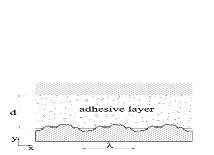
Figure 1: An elastic layer of thickness $d$ in adhesive contact with a rough periodic substrate of wavelength $\lambda$.

Fig. 2 shows, in particular, the total displacement $u_{\mathrm{tot}}$ of the substrate, the average displacement $u_{\mathrm{m}}$ of boundary of the deformed layer and the penetration $\Delta$ of the rigid substrate into the elastic slab. These three quantities are shown to satisfy the following relation

$$u_{\mathrm{tot}}=\Delta+u_{\mathrm{m}}$$ (1)

Figure 2: The definition of substrate displacement $u_{\mathrm{tot}}$, elastic layer average displacement $u_{\mathrm{m}}$, and substrate penetration $\Delta$.

We will focus on the pressure distribution $\sigma\left(x\right)$ and the displacement $u\left(x\right)$ of the elastic solid at the interface. In Refs. carbone-thickslab and Carbone G.C. has shown that the unknown pressure distribution in the contact area $\mathrm{\Omega}$ can be determined by solving the following Fredholm integral equation of the first kind with a logarithmic kernel as

$$-\int_{\mathrm{\Omega}}\mathcal{G}\left(x-s\right)\sigma\left(s\right)ds=\left[h\left(x\right)-h_{\max}\right]+\Delta;\qquad x\in\mathrm{\Omega}$$ (2)

where $\mathrm{\Omega}=\cup_{i=1}^{L}\left[a_{i},b_{i}\right]$ is the unknown contact domain to be determined as shown below. The quantities $a_{i}$ and $b_{i}$ are the unknown coordinates of $i$-th contact patch with $a_{i}<b_{i}$ and $i=1,2,...,L$, where $L$ is the unknown number of contacts. In Eq. (2), assuming the elastic layer is infinitely thick (i.e. $d\rightarrow+\infty$), the kernel is

$$\mathcal{G}\left(x\right)=\frac{2\left(1-\nu^{2}\right)}{\pi E}\log\left[2\left|\sin\left(\frac{kx}{2}\right)\right|\right]$$ (3)

and represents the Green’s function of the semi-infinite elastic body under a periodic loading, i.e. it represents the displacement $u\left(x\right)-u_{\mathrm{m}}$ caused by the application of a Dirac comb with peaks $\delta\left(x-n\lambda\right)$ separated by a distance $\lambda$. Here $E$ and $\nu$ are the Young modulus and the Poisson ratio of the elastic layer. In Eq. (2) and the quantity $h\left(x\right)$ represents the heights of the rough profile measured from its mean plane. Since we are considering a periodic problem $h\left(x\right)$ can be written as Fourier series

$$h\left(x\right)={\displaystyle\sum\limits_{m=1}^{+\infty}}h_{m}\cos\left(mq_{0}x+\phi_{m}\right)$$ (4)

where the fundamental wave vector is $q_{0}=2\pi/\lambda$. Also we have defined in Eq. (2) the quantity $h_{\max}=\max\left[h\left(x\right)\right]$, which is the maximum height of the substrate roughness. Once the pressure distribution is known the elastic displacements at the interface can be easily determined through the equations

$$u\left(x\right)-u_{\mathrm{m}} =-\int_{\mathrm{\Omega}}\mathcal{G}\left(x-s\right)\sigma\left(s\right)ds;\qquad x\in\mathrm{D}-\mathrm{\Omega}$$ (5)

$$u\left(x\right)-u_{\mathrm{m}} =h\left(x\right)-h_{\max}+\Delta;\qquad x\in\mathrm{\Omega}$$

where $\mathrm{D}=\left[-\lambda/2,\lambda/2\right]$. Of course for a infinitely thick layer ($d\rightarrow+\infty$ as in our case) the average displacement $u_{\mathrm{m}}$ is also infinitely large except when the $\nu=0.5$, but the difference $u\left(x\right)-u_{\mathrm{m}}$ is always finite carbone-thickslab , Carbone , and can be interpreted as the additional elastic displacement of the solid due to the presence of roughness at the interfaces. In order to close the system of equations we need ad additional condition to determine the yet unknown contact domain $\mathrm{\Omega}$. To this end (see also Ref. carbone-thickslab ), we first observe that for any penetration $\Delta$, we can calculate the pressure distribution at the interfaces through Eq. (2), and the interfacial elastic displacement through Eq. (5), as functions of the unknown coordinates $a_{i}$ and $b_{i}$ of the $i$-th contact area. To calculate the exact values of the quantities $a_{i}$ and $b_{i}$, given isothermal conditions, we need to find the stationary point of the free interfacial energy $U_{\mathrm{tot}}\left(a_{1},b_{1},...,a_{L},b_{L},\Delta\right)$ of the system for a fixed value of the penetration $\Delta$, this is the same as requiring that

$$\left(\frac{\partial U_{\mathrm{tot}}}{\partial a_{i}}\right)_{\Delta,b_{j}}=0,\qquad\left(\frac{\partial U_{\mathrm{tot}}}{\partial b_{i}}\right)_{\Delta,a_{j}}=0.$$ (6)

The interfacial energy (see Ref. carbone-thickslab ) is

$$U_{\mathrm{tot}}=U_{\mathrm{el}}+U_{\mathrm{ad}}$$ (7)

where we have defined the interfacial elastic energy $U_{\mathrm{el}}$ as the amount of elastic energy stored in the solid as a consequence of the elastic deformations caused by the substrate asperities i.e.

$$U_{\mathrm{el}}\left(a_{1},b_{1},...,a_{L},b_{L},\Delta\right)=\frac{1}{2}{\displaystyle\sum\limits_{i=1}^{L}}\int_{a_{i}}^{b_{i}}\sigma\left(x\right)\left[h\left(x\right)-h_{\max}+\Delta\right]dx.$$ (8)

and the adhesion energy is

$$U_{\mathrm{ad}}\left(a_{1},b_{1},...,a_{L},b_{L}\right)=-\gamma{\displaystyle\sum\limits_{i=1}^{L}}\int_{a_{i}}^{b_{i}}\sqrt{1+\left[h^{\prime}\left(x\right)\right]^{2}}dx.$$ (9)

where $\gamma$ is the Duprè energy of adhesion per unit area. Eqs. (2), (5) and (6) constitute a set of closed equations which allows, for any given penetration $\Delta$, to determine the coordinates $a_{i}$ and $b_{i}$ of each contact patch, the pressure distribution at the interface, and all other thermodynamical quantities. For the numerical implementation the reader is referred to Ref. carbone-thickslab , here we just describe some numerical techniques which are peculiar to the problem we discuss in this paper. Let us assume that we know the solution of Eqs. (6) for a given penetration $\Delta$: the knowledge of the contact region $\mathrm{\Omega}=\bigcup_{i=1}^{N}[a_{i},b_{i}]$ is sufficient to fully characterize the system. Eq. (2) determines the stress $\sigma(x)$; we solve it iteratively, through the Gauss-Seidel algorithm. Special care has been taken to guarantee stability and accuracy of the solution by choosing a suitable sampling grid: the domain $\mathrm{\Omega}$ is discretized in a non-uniform, adaptive way, so to ensure that more points are employed close to the edges of the contacts, where the stress distribution, because of adhesion, presents a square root singularity. As long as the stress is known, the deformed profile of the elastic layer follows from Eq. (5). The interfacial energy is then given by Eqs. (7), (8) and (9).

In summary, at a low level in our numerical implementation of the algorithm there is the Solver, a software code that, given the penetration and the contact regions, calculates everything else. On top of it we built another piece of software in charge to adjust the position of the contacts boundaries ${a_{1},b_{1},\ldots,a_{N},b_{N}}$ so to minimize the interfacial energy. We employed a conjugate gradient method in the version given by Polak and Ribiére Conj-Grad . Unfortunately the problem is more complex than a minimization in a $2N$-dimensional space. Starting form an arbitrary configuration, some of the contact boundaries can acquire the same value, meaning that either a contact is detaching or two contacts are coalescing together into a single bigger one. If this happens, the minimization has to be restarted in a different number of dimensions.

Furthermore, a constraint must be accounted: in principle we can determine the configuration corresponding to any penetration and contacts, but we must impose that in the non-contact regions the elastic layer never intersects the substrate. For instance, if we consider a physical configuration minimizing the interfacial energy, and then we increase the penetration pushing the substrate against the elastic layer, the starting point for the new conjugate gradient minimization may show an intersection between the elastic layer and some peaks of the substrate in the non-contact regions. This indicates that a new contact has to be added before starting the minimization. A specific procedure inside our software is in charge to detect all the intersections between elastic layer and substrate, so to enforce the physical constraints of the problem. Given the penetration $\Delta$, the search of the contact domain $\mathrm{\Omega}$ that minimizes the interfacial energy is challenging: not only the $2N$ variables ${a_{1},b_{1},\ldots a_{N},b_{N}}$ are unknown, but also the number $N$ of contact regions is unknown! The solution of the problem resorts to conjugate gradient minimization alternated to searches for intersections between the elastic layer and the block. The minimization procedure stops when the conjugate gradient ends successfully, i.e. it is not interrupted by a coalescence of detachment of contacts, and the successive search for intersections confirms that there are no intersections in the non-contact regions. Although we took special care to guarantee that the minimization procedure would converge for moderately large variations of penetration, we observed that the most reliable approach involves many small increments of penetration starting from 0 (non-contact) up to desired value, while optimizing of the solution at every intermediate step. The solution of the contact problem in presence of adhesion is not unique, that is, for the same penetration more configurations are possible depending on the loading history. Nonetheless the contact pattern occurring with increasing penetration is uniquely identified and it is the most suitable solution to represent the non-adhesive contact in the limit of vanishingly small adhesive bonds. As a final remark, we observe that this algorithm cannot be used to solve the problem without adhesion: in this case the solution is still a stationary point satisfying Eq. (6), but the profile of the elastic layer in the non-contact regions is always tangent to the substrate near the crack tips $a_{i}$ and $b_{i}$. An infinitesimal motion of any of the crack points decreasing the contact region would cause an intersection between elastic layer and substrate. In other terms, the solution lies always on the boundary of the subset of $\mathbb{R}^{2N}$ identified by the physical constraint of non-intersection. The solution would not be a minimum without such a constraint.

III Persson’s theory for anisotropic surfaces

The aim of this paper is to compare the numerical results with analytical predictions of one of the most promising and also strongly debated theory of contact mechanics, i.e. the recent theory by Persson Person Rubb Fric JCP , PerssonAdhesion . However, the surface we are considering is strongly anisotropic, in fact it is rough in only one direction and smooth in the orthogonal direction. The original theory proposed by Persson was, instead, conceived and developed for perfectly isotropic surfaces. Therefore in order to carry out the analysis we need to extend this theory to the case of anisotropic surfaces. This extension has been obtained in Ref. carbone Persson anysotropu . Here we briefly summarize the main equations. Persson’s theory removes the assumption, which is implicit in the multiasperity contact theories, that the area of real contact is small compared to the nominal contact area. On the contrary, Persson focuses on the probability distribution $P\left(\sigma,\zeta\right)$ of normal stresses at the interface, which depends on the magnification at which the contact interface is observed. To calculate the governing equation of $P\left(\sigma,\zeta\right)$, Persson moves from the limiting case of full contact conditions between a rigid rough surface and an initially flat elastic half-space Person Rubb Fric JCP . In such conditions the PSD of the deformed elastic surface is equal to $C_{\mathrm{2D}}\left(\mathbf{q}\right)$ where $C_{\mathrm{2D}}\left(\mathbf{q}\right)=\left(2\pi\right)^{-2}\int d^{2}x\left\langle h\left(\mathbf{0}\right)h\left(\mathbf{x}\right)\right\rangle e^{-i\mathbf{q}\cdot\mathbf{x}}$ is the PSD of the rigid rough substrate (the quantity $h\left(\mathbf{x}\right)$ is the rough substrate height distribution, $\mathbf{x=}\left(x,y\right)$ is the in-plane position vector and the symbol $\left\langle{}\right\rangle$ stands for the ensemble average). Considering that for a perfectly elastic material the elastic modulus is frequency independent, it can be easily shown (see Ref. carbone Persson anysotropu ) that even for the general case of anisotropic surfaces Persson’s theory states that the stress probability distribution $P\left(\sigma,\zeta\right)$ must satisfy the following relation.

$$\frac{\partial P\left(\sigma,\zeta\right)}{\partial\zeta}=f\left(\zeta\right)\frac{\partial^{2}P\left(\sigma,\zeta\right)}{\partial\sigma^{2}}$$ (10)

where the magnification $\zeta=q/q_{0}$, and $\sigma$ is the interfacial stress in the apparent contact area at the magnification $\zeta$. The diffusivity function $f\left(\zeta\right)=q_{L}G^{\prime}\left(q\right)\sigma_{0}^{2}$, where $\sigma_{0}$ is the the average normal stress in the contact area and $G\left(q\right)$ is calculated in full contact conditions as

$$G(q)={\frac{1}{8}}\left({\frac{E}{1-\nu^{2}}}\right)^{2}\frac{1}{\sigma_{0}^{2}}\langle[\nabla h(\mathbf{x})]^{2}\rangle_{q}$$ (11)

where

$$\langle[\nabla h(\mathbf{x})]^{2}\rangle_{q}=\int_{\left|\mathbf{q}^{\prime}\right|<q}d^{2}q^{\prime}\ q^{\prime 2}C(\mathbf{q}^{\prime})$$ (12)

is the mean square value of the slope when the surface is observed at the magnification $\zeta=q/q_{0}$, that is when all harmonic components of the spectrum with wavevector above $q$ are filtered out. Then, Persson assumes that Eqs. (10) and (11) hold true also in partial contact (this is of course an approximation since the PSD of the deformed surface in partial contact conditions cannot be the same as that of the rigid rough substrate) and to account for partial contact the following initial and boundary conditions are enforced

$$P\left(\sigma,1\right) =\delta\left(\sigma-\sigma_{0}\right)$$

$$P\left(-\sigma_{\mathrm{a}},\zeta\right) =0$$ (13)

$$P\left(\infty,\zeta\right) =0$$

Here $\sigma_{\mathrm{a}}\left(\zeta\right)$ is the tensile stress needed to cause detachment over a strip of length $2\pi/q$, recalling the Griffith criterion in plain strain Griffith we get

$$\sigma_{\mathrm{a}}\left(\zeta\right)=\left[\frac{2}{\pi^{2}}E^{\ast}\gamma_{\mathrm{eff}}\left(\zeta\right)q\right]^{1/2}$$ (14)

where $E^{\ast}=E/\left(1-v^{2}\right)$. In Eq. (14) the quantity $\gamma_{\mathrm{eff}}\left(\zeta\right)$ is the apparent energy of adhesion at the interface defined as PerssonAdhesion , carbone mang pers

$$-\gamma_{\mathrm{eff}}\left(\zeta\right)A\left(\zeta\right)=U_{\mathrm{ad}}\left(\zeta\right)+U_{\mathrm{el}}\left(\zeta\right)$$ (15)

where $A\left(\zeta\right)$ is the apparent contact area at the magnification $\zeta$. The calculation of the elastic energy $U_{\mathrm{el}}\left(\zeta\right)$ must take into account that because of partial contact conditions the elastic energy stored at the interface is less than what would be stored in case of full-contact conditions. This is necessarily true because only where contact occurs the elastic solid conforms the underlying substrate, whereas outside of the contact regions the elastic surface is much less deformed. Persson accounts for this fact by assuming that, when calculating the interfacial elastic energy $U_{el}$, the PSD of the deformed (initially flat) elastic surface is equal to $C_{\mathrm{2D}}\left(\mathbf{q}\right)A\left(q\right)/A_{0}$ where $A\left(q\right)/A_{0}$ is the fraction of apparent contact area at the length scale $2\pi/q$ i.e.

$$U_{\mathrm{el}}\left(\zeta\right)=\frac{1}{4}E^{\ast}\int_{\left|\mathbf{q}\right|>\zeta q_{0}}d^{2}qqC_{\mathrm{2D}}\left(\mathbf{q}\right)A\left(q\right)$$ (16)

This result, that at the beginning was only conjectured by Persson Person Rubb Fric JCP , recently has been demonstrated to directly follow from Persson’s theory itself persson PSD stress . Analogously the adhesion energy $U_{\mathrm{ad}}\left(\zeta\right)$ is calculated as

$$U_{\mathrm{ad}}\left(\zeta\right)=-\gamma A\left(\zeta_{\max}\right)\int_{0}^{\infty}dx\left(1+\xi^{2}x\right)^{1/2}e^{-x}$$ (17)

where

$$\xi^{2}=\int_{\left|\mathbf{q}\right|>\zeta q_{0}}d^{2}qq^{2}C_{\mathrm{2D}}\left(\mathbf{q}\right)$$

and $\zeta_{\max}=q_{1}/q_{0}$, $q_{0}=2\pi/\lambda$, and $q_{1}=2\pi/\lambda_{1}$ where $\lambda_{1}$ is the shortest length scale of the rough surfaces. Equations (10, 13, 14, 15, 16 and 17) can be solved to calculate the stress probability distribution $P\left(\sigma,\zeta\right)$ and hence the apparent contact area $A\left(\zeta\right)/A_{0}$ as a function of the magnification $\zeta$ PerssonAdhesion , carbone mang pers

$$\frac{A\left(\zeta\right)}{A_{0}}=\int_{-\sigma_{a}\left(\zeta\right)}^{\infty}P\left(\sigma,\zeta\right)d\sigma$$ (18)

The separation $s=h_{\max}-\Delta$ can be calculated observing that the change of total interfacial energy $U_{\mathrm{tot}}=U_{\mathrm{el}}+U_{\mathrm{ad}}$ must be equal to the work done by the applied load, i.e.

$$dU_{\mathrm{tot}}=\sigma_{0}A_{0}d\Delta=-\sigma_{0}A_{0}ds$$ (19)

which gives

$$s=\int_{\sigma_{0}}^{+\infty}\frac{1}{A_{0}\sigma_{0}^{\prime}}\frac{dU_{\mathrm{tot}}}{d\sigma_{0}^{\prime}}d\sigma_{0}^{\prime}$$ (20)

In case of non-adhesive contact i.e. when $\gamma=0$, Persson has shown that

$$P\left(\sigma,\zeta\right)=\frac{1}{2\left(\pi G\right)^{1/2}}\left[e^{-\left(\sigma-\sigma_{0}\right)^{2}/4G}-e^{-\left(\sigma+\sigma_{0}\right)^{2}/4G}\right]$$ (21)

and Eq. (18) simply becomes

$$\frac{A\left(\zeta\right)}{A_{0}}=\operatorname{erf}\left({\frac{1}{2\surd G(\zeta)}}\right)$$ (22)

The above formulation holds true also for anisotropic surfaces, in particular if the substrate has roughness in only one direction, e.g. along the $x$-direction, we get $\left\langle\left[\nabla h(\mathbf{x})\right]^{2}\right\rangle_{q}=\left\langle\left(\partial h/\partial x\right)^{2}\right\rangle_{q}$. In such a case we have $h(\mathbf{x})=h(x)$ and one can easily show that

$$C_{\mathrm{2D}}(\mathbf{q})=C(q_{x})\delta(q_{y})$$ (23)

where $C\left(q\right)=\left(2\pi\right)^{-1}\int dx\left\langle h\left(0\right)h\left(x\right)\right\rangle e^{-iqx}$ is the PSD of the $x$-profile of the surface. Using Eq. (23) one simply obtains

$$\left\langle\left(\partial h/\partial x\right)^{2}\right\rangle_{q}=\int_{-q}^{q}dq_{x}q_{x}^{2}C(q_{x})$$ (24)

Eq. (18) gives the apparent contact area at the resolution $\lambda\left(q\right)=2\pi/q$ as a function of the applied load $\sigma_{0}$. However, we are interested in calculating the real contact area, which can be obtained by replacing $\zeta$ with $\zeta_{\max}$.

IV Rough profile generation

In order to carry out the numerical simulations and compare the results with the theoretical predictions, we need to numerically generate a rough profile. We have opted for a fractal self affine rough profile. For any self affine fractal profile $h\left(x\right)$ the statistical properties are invariant under the transformation

$$x\rightarrow tx;\qquad h\rightarrow t^{H}h$$ (25)

in such a case it can be shown that the PSD of the profile is

$$C\left(q\right)=C_{0}\left(\frac{\left|q\right|}{q_{0}}\right)^{-\left(2H+1\right)}$$ (26)

where $H$ is the Hurst exponent of the randomly rough profile, and is related to the fractal dimension $D_{f}=2-H$. In order to carry out the numerical calculations we have utilized a periodic profile with Fourier components up to the value $q_{1}=Nq_{0}$ (in this case $\zeta_{1}=N$). However we need to determine the amplitudes $h_{m}$ and the phases $\phi_{m}$ of the harmonic terms [see Eq. (4)]. It can be shown that in order to satisfy the translational invariance of the profile’s statistical properties (which implies that the autocorrelation function satisfies the relation $\left\langle h\left(x^{\prime}\right)h\left(x^{\prime}+x\right)\right\rangle=\left\langle h\left(0\right)h\left(x\right)\right\rangle$), it is enough to assume that the random phases $\phi_{m}$ are uniformly distributed on the interval $\left[-\pi,\pi\right[$. In such a case the autocorrelation of the profile takes the form

$$\left\langle h\left(x^{\prime}\right)h\left(x^{\prime}+x\right)\right\rangle={\displaystyle\sum\limits_{m=1}^{N}}\frac{\left\langle h_{m}^{2}\right\rangle}{2}\cos\left(mq_{0}x\right)$$ (27)

Now we need to calculate the quantities $\left\langle h_{m}^{2}\right\rangle$. To this purpose let us calculate the PSD of the periodic profile of Eq. (4). By using the definition we get

$$C\left(q\right)=\left(2\pi\right)^{-1}{\displaystyle\sum\limits_{m=1}^{N}}\int dx\frac{\left\langle h_{m}^{2}\right\rangle}{2}\cos\left(mq_{0}x\right)e^{-iqx}={\displaystyle\sum\limits_{m=1}^{N}}\frac{1}{4}\left[\left\langle h_{m}^{2}\right\rangle\delta\left(q-mq_{0}\right)+\left\langle h_{m}^{2}\right\rangle\delta\left(q+mq_{0}\right)\right]$$ (28)

from which it follows that

$$C\left(-mq_{0}\right)=C\left(mq_{0}\right)=C_{m}=\frac{\left\langle h_{m}^{2}\right\rangle}{4}\delta\left(0\right)$$

Using Eq. (26) and observing that $\ C_{0}=\left\langle h_{1}^{2}\right\rangle\delta\left(0\right)/4$, one then obtains

$$\left\langle h_{m}^{2}\right\rangle=\left\langle h_{1}^{2}\right\rangle m^{-\left(2H+1\right)}$$ (29)

Hence, the quantity $\left\langle h_{m}^{2}\right\rangle$ can be determined once known $\left\langle h_{1}^{2}\right\rangle$ and the Hurst exponent of the surface.

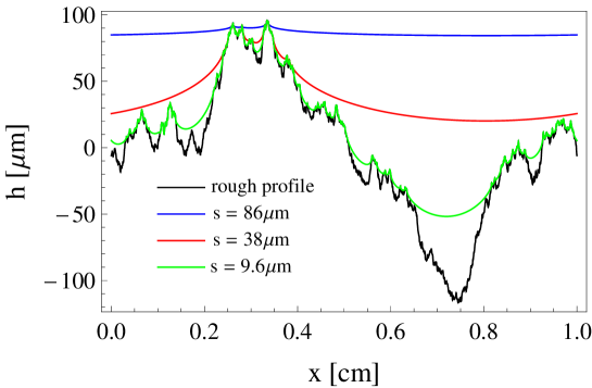
Figure 3: The deformed shape of the elastic body at three different separations, $s=86\mathrm{\mu m}$ (blue), $s=48\mathrm{\mu m}$ (red), and $s=9.6\mathrm{\mu m}$ (green). The rough rigid substrate profile is shown in black color.

Now observe from Eq. (27) that $\left\langle h\left(x\right)^{2}\right\rangle=\sum_{m=1}^{N}\left\langle h_{m}^{2}\right\rangle/2$, and using Eq. (29) one obtains

$$\left\langle h\left(x\right)^{2}\right\rangle=\frac{\left\langle h_{1}^{2}\right\rangle}{2}\sum_{m=1}^{N}m^{-\left(2H+1\right)}$$ (30)

Therefore, if one knows the rms roughness of the surfaces $h_{\mathrm{rms}}=\sqrt{\left\langle h\left(x\right)^{2}\right\rangle}$ one can calculate $\left\langle h_{1}^{2}\right\rangle$ and therefore all the other quantities $\left\langle h_{m}^{2}\right\rangle$. However to completely characterize the rough profile we still need the probability distribution of the amplitudes $h_{m}$. There are several choices, however the simplest assumption, as suggested by Persson et al. in Ref. Persson Roughness , is that the probability density function of $h_{m}$ is just a Dirac’s delta function centered at $\left[4C_{m}/\delta\left(0\right)\right]^{1/2}\approx 2\sqrt{2\pi}C_{m}^{1/2}/L^{1/2}$, i.e.

$$p\left(h_{m}\right)=\delta\left(h_{m}-2\sqrt{\frac{2\pi}{L}}C_{m}^{1/2}\right)$$ (31)

where we have used that $\delta\left(q=0\right)\approx L/\left(2\pi\right)$. In can be shown Persson Roughness that this choice guarantees also that the random profile $h\left(x\right)$ has a Gaussian random distribution.

V Results

We assume that the elastic block is a soft perfectly elastic material with elastic modulus $E=1\mathrm{MPa}$ and Poisson’s ratio $\nu=0.5$, i.e. we assume that the material is incompressible. We assume also that the change of surface energy upon contact between the two surfaces (i.e. the Duprè energy of adhesion) is $\gamma=0.03\mathrm{J/m}^{2}$. Calculations have been carried out for 11 different realizations of a rough self-affine fractal 1D profile.

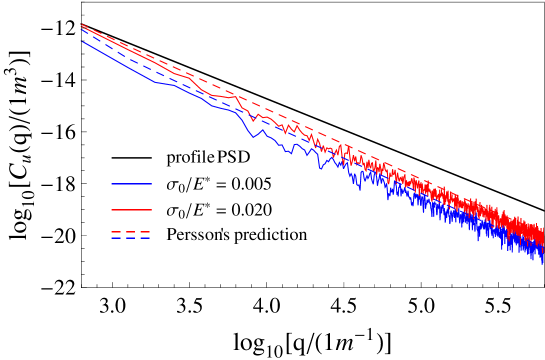
Figure 4: The PSD $C_{u}\left(q\right)$ of the rigid substrate profile (black solid line) compared to that of the deformed shape of the elastic body for two different dimensionless loads $\sigma_{0}/E^{\ast}=0.005$ (blue), and $\sigma_{0}/E^{\ast}=0.020$ (red). Solid lines refer to numerical calculations whereas dashed lines refer to Persson’s theory. The agreement between Persson’s theory and numerical calculated predictions is qualitatively very good. Indeed the slope of the PSD predicted by Persson (in the mid range of $q$-vectors where the influence of adhesion is negligible) is almost the same as the numerically calculated one (see text): in both cases the PSD of the elastically deformed solid is $C_{u}\left(q\right)\approx q^{-\left(2+H\right)}$.

The profile has a fractal dimension $D_{f}=1.3$ (i.e. the Hurst coefficient is $H=0.7$), with root mean square roughness $\left\langle h^{2}\right\rangle^{1/2}=50\mathrm{\mu m}$. The self-affine profiles have spectral components in the range $q_{0}<q<q_{1}$. We have used $\lambda=2\pi/q_{0}=0.01\mathrm{m}$ and $q_{1}=10^{3}q_{0}$. The numerical calculations have been carried out for different values of the separations $s=h_{\max}-\Delta$, which is defined as the distance between the mean plane of the deformed surface and the mean plane of the rough surfaces. In Fig. 3 we show three different shapes of the deformed profiles at three different values of the separation: $s=86\mathrm{\mu m}$ (blue), $s=38\mathrm{\mu m}$ (red), and $s=9.6\mathrm{\mu m}$ (green). The black line instead represents the rigid rough substrate profile. A deeper analysis of the figure shows that, not depending on the separation $s$, full contact occurs between the elastic block and the short wave length corrugation of the rough rigid profile.

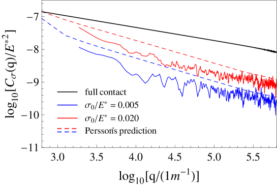
Figure 5: The quantity $C_{\sigma}\left(q\right)/E^{\ast 2}$ for full contact conditions (black solid line) and for two different dimensionless loads $\sigma_{0}/E^{\ast}=0.005$ (blue), and $\sigma_{0}/E^{\ast}=0.020$ (red). Solid lines refer to numerical calculations whereas dashed lines refer to Persson’s theory. Also in this case the agreement between Persson’s theory and numerical calculated predictions is qualitatively very good, at least in the mid range of $q$-vectors where the influence of adhesion is negligible: both calculations predict $C_{\sigma}\left(q\right)\approx q^{-H}$.

This is in agreement with some theoretical arguments PerssonAdhesion , carbone mang pers which predict that this situation should occur when the Hurst exponent of the rough profile is larger than 0.5, as in our case. This is also confirmed in Fig. 4 which shows the PSD of the rough surface and that of the deformed elastic surface as a function of the wave-vector $q$ (in a log-log diagram) for two values of the applied stress $\sigma_{0}/E^{\ast}=0.005$ (blue), and $\sigma_{0}/E^{\ast}=0.020$ (red), where $E^{\ast}=E/\left(1-\nu^{2}\right)$. Indeed, we observe that for large $q$-vectors the PSD $C_{u}\left(q\right)=\left(2\pi\right)^{-1}\int dx\left\langle u\left(0\right)u\left(x\right)\right\rangle e^{-iqx}$ of the numerically calculated deformed profile $u\left(x\right)$ becomes almost perfectly parallel to the PSD $C\left(q\right)$ of the rigid substrate: this means that the spectral content of the deformed body profile at short wavelength is just the same as that of the rough rigid profile, and therefore that full contact occurs between the elastic body and the substrate at short wavelengths. Fig. 4, shows also, as expected, that, as the load is increased, the quantity $C_{u}\left(q\right)$ continuously approaches the PSD $C\left(q\right)$ of the rigid rough profile and must become equal to $C\left(q\right)$ at very high loads, i.e. when full contact occurs.

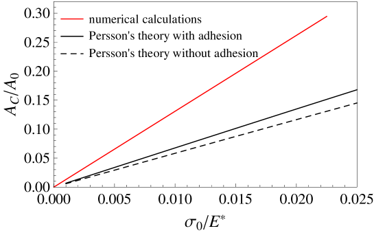
Figure 6: The true contact area $A\left(\zeta_{\max}\right)$ in units of the the nominal contact area $A_{0}$ as a function of the dimensionless applied load $\sigma_{0}/E^{\ast}$. Numerical predictions are in red, whereas Persson’s theoretical calculations are in black colour. Observe that both numerical calculations and Persson’s theory predict linearity between contact area and load. However Persson’s theory predicts a coefficient of proportionality which is about half of the numerically calculated one. The dashed line represents Persson’s calculations in absence of adhesion interactions. Notice that because of the low amount of adhesion the curve does not differ significantly from the solid line.

In Fig. 4 we also compare the numerically calculated PSD of the deformed surface (solid line) with Persson’s theoretical predictions (dashed line). We first observe that there is a non negligible shift between Persson’s results and our numerically calculated ones. However the two curves run almost perfectly parallel especially in the mid range of wavevectors where the best fit of our numerical results gives $C_{u}\left(q\right)\approx q^{-2.73}$. The value $-2.73$ is very close to the value $-2.7$ predicted by Persson. Indeed, Persson’s theory relies on the assumption that the PSD of the deformed surfaces $C_{u}\left(q\right)=C\left(q\right)A\left(q\right)/A_{0}$, where $C\left(q\right)$ is the PSD of the rough substrate. Now, in case of self affine fractal surfaces, using Eq. (26) and observing that if one neglects adhesion (this is correct in the mid range of wavevectors $q$) Eqs. (11) and (22) give $A\left(q\right)/A_{0}\approx q^{H-1}$, one obtains from Persson’s theory that $C_{u}\left(q\right)\approx q^{-\left(2+H\right)}$. Being, in our case, $H=0.7$, we have $C_{u}\left(q\right)\approx q^{-2.7}$in perfect agreement with our numerical calculations.

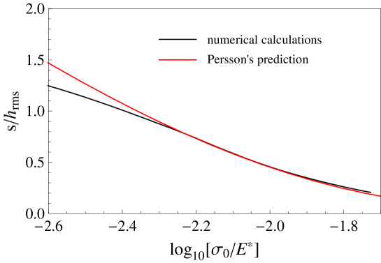
Figure 7: The separation $s$ in units of roughness $h_{\mathrm{rms}}$ as a function of the dimensionless applied load $\sigma_{0}/E^{\ast}$ in a log-linear scale. The agreement between numerical data (black curve) and the Persson’s theoretical predictions (red curve) is almost perfect. The numerical calculations deviate from theoretical predictions only at small loads, since our system is a finite system so a finite value of the separation $s$ necessarily exists at which contact area goes to zero and therefore also the applied load. Persson’s theory instead has been developed for infinite systems. In this case indeed the rough surface has arbitrarily many and arbitrarily high asperities, which always allows the contact between the two solids to occur for arbitrarily large surface separations.

Same conclusions can be found if one observes Fig. 5 which shows in a log-log diagram the power spectral density $C_{\sigma}\left(q\right)=\left(2\pi\right)^{-1}\int dx\left\langle\sigma\left(0\right)\sigma\left(x\right)\right\rangle e^{-iqx}$ of the stress distribution at the interface in units of $E^{\ast 2}$. Of course this is not unexpected since the $C_{\sigma}\left(q\right)$ and $C_{u}\left(q\right)$ are related each-other through $C_{\sigma}\left(q\right)=\frac{1}{4}E^{\ast 2}q^{2}C_{u}\left(q\right)$ persson PSD stress , carbone Persson anysotropu . Using that $C_{u}\left(q\right)\approx q^{-\left(2+H\right)}$, and assuming the adhesion interaction is not important (which occurs in the mid range of wavevectors $q$), one obtains, $C_{\sigma}\left(q\right)\approx q^{-H}$. This is indeed confirmed in Fig. 5 which shows that Persson’s prediction (dashed lines) and numerical calculations (solid lines) run parallel to each other in low-mid range of $q$-vectors. However, as $q$ is increased the numerical calculated PSD $C_{\sigma}\left(q\right)$ rapidly changes its slope.

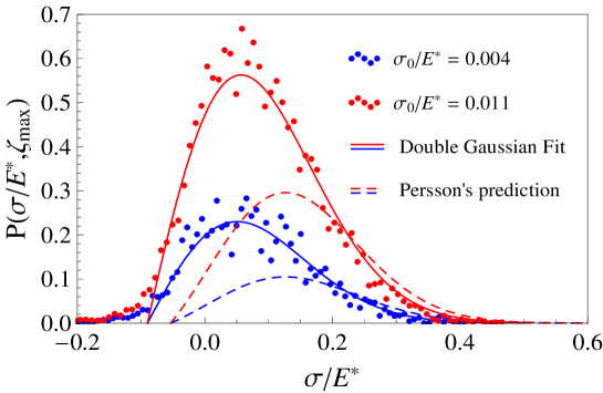
Figure 8: The probability function $P\left(\sigma,\zeta_{\max}\right)$ of interfacial pressure distribution $\sigma\left(x\right)$. Points are numerical predictions whereas dashed lines are Persson’s results. The trend is qualitatively the same, although it is quantitatively different. The reason for such a difference is that numerical calculations and Persson’s theory do not predict the same value of the contact area for any given applied load (see Fig. 6). Notice that, the tail of numerically calculated probability distribution at negative loads is an effect of the adhesion interaction which has been introduced only through the surface energy, i.e. with the inclusion of an interaction force with an infinitesimally short range. We also present a best fit based on double Gaussian probability distribution (see text).

This, in turn, becomes almost equal to that of the PSD of interfacial normal stress distribution that would be obtained in full contact conditions (solid black line in Fig. 5), and confirms, what we have already observed above, i.e. that because of adhesion the short wavelength roughness of the underlying rigid profile is in full contact with the elastic body. Figure 6 shows the true contact area $A\left(\zeta_{\max}\right)/A_{0}$ vs. the dimensionless load $\sigma_{0}/E^{\ast}$ calculated through Persson’s theory for adhesive contact and the one computed by our numerical code. Figure 6 confirms the linearity between contact area and load, however it also shows a significant disagreement between Persson’s theory and our numerical calculations. In particular, Persson’s theory predicts a contact area which is about 50% less than that calculated with our numerical code, in agreement with some molecular dynamics simulations Yang-Persson , where Persson himself has found a difference between the numerically calculated contact area and the theoretical value of about 30% for a two-dimensional rough surface. The dashed curve in Fig. 6 represents Persson’s theoretical predictions when adhesion is not included in calculations. As expected adhesive interactions lead to an increase of the contact area.

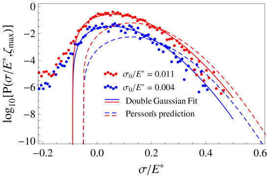
Figure 9: The logarithm of the probability function $P\left(\sigma,\zeta_{\max}\right)$. Points are numerical predictions whereas dashed lines are Persson’s results. We observe that the tail of the probability distribution at large values of $\sigma$ follow exactly a Gaussian distribution, whereas the tail obtained for negative value of $\sigma$ is not Gaussian.

However, being in our case the amount of adhesion energy relatively small, this effect is only marginal. We observe that the large discrepancy between Persson’s predictions and our numerical calculations may be explained, at least partially, by the fact that Persson’s theory is a mean field theory in spirit, so it should work better for 2D rough surfaces rather than for 1D rough surfaces. Fig. 7 shows the dimensionless separation $s/h_{\mathrm{rms}}$ as a function of the dimensionless load $\sigma_{0}/E^{\ast}$. Numerical predictions (black line) are compared to Persson’s ones. The agreement is very good except at lower applied loads. Indeed at small loads the numerically calculated separation drops off faster than predicted by Persson’s theory. The same effect has also been observed in molecular dynamics calculations Yang-Persson . The explanation for this behavior is that numerical calculations have been carried out for a finite system, whereas Persson’s theory is for an infinite system. Indeed an infinite system has many (arbitrarily) high asperities, which always allows the contact between the two solids to occur for arbitrarily large surface separations. But a finite system has asperities with height below some finite length $h_{\max}$, and for $u>h_{\max}$ no contact occurs between the solids and $\sigma_{0}\rightarrow 0$. Fig. 8 shows the probability density function $P\left(\sigma,\zeta_{\max}\right)$ of interfacial normal stress distribution $\sigma\left(x\right)$ at the highest magnification. We observe that Persson’s predictions and numerical data agree only at a qualitative level, but strongly deviates from a quantitative point of view. The reason of this quantitative disagreement can be easily understood if one recalls Eq. (18) which states that the integral of the $P\left(\sigma,\zeta_{\max}\right)$ must be proportional to the true contact area $A\left(\zeta_{\max}\right)$ and considers that Persson’s theory predicts a contact area smaller by a factor $\approx 1/2$, if compared to numerical calculations. We also present with solid lines the best fit obtained with the double Gaussian distribution

$$P\left(\sigma,\zeta_{\max}\right)=\frac{1}{2\left(\pi G\right)^{1/2}}\left[e^{-\left(\sigma-\sigma_{0}+\sigma_{\mathrm{a}}\right)^{2}/4G}-e^{-\left(\sigma+\sigma_{0}+\sigma_{\mathrm{a}}\right)^{2}/4G}\right]$$ (32)

where we have relaxed the quantities $\sigma_{\mathrm{a}}$ and $G$. Fig. 8 and even more 9 show that, at least when the amount of adhesion energy is small (as in our case), Eq. (32) is a good approximation of the numerically calculated stress probability function $P\left(\sigma,\zeta_{\max}\right)$. Indeed Fig. 9 shows that, at high values of $\sigma$, the tail of the stress probability density function is Gaussian. Notice that, the tail of numerically calculated stress probability distribution at negative loads is an effect of the adhesion interaction which has been introduced only through the surface energy, namely by means of an interaction force with an infinitesimally short range. This even allows that infinite negative values of $\sigma$ can occur at the interface. We also observe that the value of $\sigma_{\mathrm{a}}$ calculated by fitting the interfacial stress probability density function differs from that calculated in the spirit of Persson’s theory through Eq. (14). However, it is possible to show that a better estimation of the tensile stress $\sigma_{\mathrm{a}}$, can be obtained by assuming in Eq. (14) that the width of the detached region is a factor 1/2 smaller than that originally assumed in Persson’s theory PerssonAdhesion . In such a case the estimated tensile stress $\sigma_{\mathrm{a}}$ would increase of roughly a factor 1.4 thus making $\sigma_{\mathrm{a}}$ closer to the value we have found in Fig. 8.

VI Conclusions

The authors have carried out detailed numerical calculations to determine the contact area, the stress distribution, the penetration and elastic deformation of an infinitely thick layer in adhesive contact with a rough strongly anisotropic rigid surface. The numerical predictions have been compared in detail with those of an extended version of Persson’s theory able to deal with adhesive contact between anisotropic rough surfaces. It is shown that, for any given load, the value of true contact area predicted by Persson’s theory significantly differs from the numerically calculated ones, the first being smaller by a factor $\approx 1/2$. This may also depend on the fact the Persson’s theory is of the mean-field type and, therefore, should work well in higher dimensions than in 1D. However, the predicted value of separation matches almost perfectly the numerical data. We have also compared the power spectral density of the deformed elastic surface and of the stress distribution at the interface as obtained by numerical calculations and Persson’s theory. We observe that both theory and numerical calculations predict the PSDs to follow a power law with almost the same exponents. This extends to the case of adhesive contact, what has been found previously for adhesionless contact by other authors. However, we also observe, in agreement with Persson’s theory of adhesive contact, that at high magnification the exponent of the power law changes in such a way to suggest that the elastic solid lies in full contact condition with the fine microstructure of the rough surfaces. We conclude that, Persson’s theory is able to capture the main physics behind contact mechanics of rough surfaces independently of whether adhesion is present or not. However, we also observe that from an engineering point of view a better estimation of the contact area would be very useful in practical applications as in case tires, mixed lubricated interfaces, and seals, where the kinetic friction or the amount of leakage should be accurately predicted for design purposes. Therefore an improvement of the theory, which allows to better estimate the real contact area, would be strongly appreciated by engineering community.

- (1) Yang C., Tartaglino U., and Persson B. N.J., The European Physical Journal E - Soft Matter, 19 (1), 47-58 (2006).
- (2) Borri-Brunetto M., Chiaia B., and Ciavarella M., Comput.Methods Appl. Mech. Eng. 190, 6053 (2001).
- (3) Hyun S., Pei L., Molinari J.-F., and Robbins M. O., Phys. Rev. E 70, 026117 (2004).
- (4) Campañá C., Physical Review E, 78 (2), 026110 (2008)
- (5) Greenwood J.A., Williamson J.B.P., Proc. R. Soc. London A 295, 300 (1966).
- (6) Bush A.W., Gibson R.D., Thomas T.R., Wear 35, 87 (1975).
- (7) Thomas T.R., Rough Surfaces (chap. 8), Longman Group Limited, New Yorl (1982).
- (8) Greenwood J.A., Wear 261 191-200 (2006).
- (9) Carbone G., the Journal of the Mechanics and Physics of Solids, 57 (7), 1093–1102 (2009).
- (10) Persson B.N.J., J. Chem. Phys. 115, 3840 (2001).
- (11) Persson B.N.J., Eur. Phys. J. E 8, 385 (2002).
- (12) Carbone G. , Bottiglione F., the Journal of the Mechanics and Physics of Solids 56 (8), 2555-2572 (2008).
- (13) Campañà C., Müser M. H., Robbins M. O., J. Phys.: Condens. Matter 20, 354013 (2008).
- (14) Yang C., Persson B.N.J., Physical Review Letters, 100, 024303, 2008.
- (15) Persson B.N.J., J. Phys.: Condens. Matter 20 (31) 312001 (2008).
- (16) Carbone, Lorenz B., Persson B.N.J., Wohlers A, The European Physical Journal E, 29 (3), 275–284, (2009).
- (17) Campañá C., Müser M. H., Physical Review B 74 (7), 075420 (2006)
- (18) Carbone G., Mangialardi L., The Journal of the Mechanics and Physics of Solids, 56 (2), 684-706 (2008).
- (19) Carbone G. and Mangialardi L., Journal of the Mechanics and Physics of Solids 52 (6), 1267-1287 (2004).
- (20) Polak E., Ribière G., Revue Française d’Informatique et de Recherche Opérationelle, 16, 35–43 ( 1969).
- (21) Carbone G., Mangialardi L., Persson B.N.J., Phys. Rev. B 70, 125407 (2004).
- (22) Griffith A.A., Phil. Trans. Roy. SOc. A 221, 163 (1920).
- (23) Persson B. N. J., Albohr O., Tartaglino U., Volokitin A. I., Tosatti E., J. Phys.: Condens. Matter 17 R1–R62 (2005).