Effects of dissipation in an adiabatic quantum search algorithm

Abstract

We consider the effect of two different environments on the performance of the quantum adiabatic search algorithm, a thermal bath at finite temperature, and a structured environment similar to the one encountered in systems coupled to the electromagnetic field that exists within a photonic crystal. While for all the parameter regimes explored here, the algorithm performance is worsened by the contact with a thermal environment, the picture appears to be different when considering a structured environment. In this case we show that, by tuning the environment parameters to certain regimes, the algorithm performance can actually be improved with respect to the closed system case. Additionally, the relevance of considering the dissipation rates as complex quantities is discussed in both cases. More particularly, we find that the imaginary part of the rates can not be neglected with the usual argument that it simply amounts to an energy shift, and in fact influences crucially the system dynamics.

1 Introduction

The paradigm of Adiabatic Quantum Computation (AQC), introduced in [1], is known to be equivalent to standard, circuit based, quantum computation [2]. From the point of view of its physical implementation, it is however specially appealing, since it is entirely formulated in terms of a controlled dynamics, and moreover it offers some inherent robustness to errors [3].

In AQC the solution of a computational problem is encoded in the ground state of a certain (problem) Hamiltonian. The system is started in the easily preparable ground state of an initial Hamiltonian, which is then slowly turned into the problem one. The adiabatic theorem [4, 5, 6, 7, 8] guarantees that, if the variation of the Hamiltonian is sufficiently slow, time evolution will drive the system into the solution state. The resource measuring the computational cost of the algorithm is thus the total evolution time required to guarantee the adiabaticity condition. For most cases, it depends on the inverse squared of the minimum energy gap during the evolution.

Since quantum systems are not in general completely isolated from their environment, errors and dissipation are ubiquitous, and it is fundamental to decide how quantum computers and algorithms can be built that achieve their computational tasks in spite of inaccurate operations and certain loss of coherence. But AQC gets affected by errors in a fundamentally different way than the standard, gate-based model of quantum computation. The interaction with the environment may excite the system out of its ground state, causing errors, but if the energy scales in the environment are much smaller than the minimum gap, the adiabatic evolution will be naturally preserved. On the other hand, the dissipation may also result in a modified effective Hamiltonian, and thus affect the performance of the AQC [9, 10, 11]. Even when the coupling with the environment is weak, it may produce noticeable effects in the performance of the adiabatic algorithm, specially considering the large time scales that this requires.

Looking at the question from a different perspective, the algorithm may be implemented within a system inwhich the interaction with the environment is not an undesirable effect, but rather a tool that can be actually controlled and tuned at will to improve the performance of AQC. Whether the effect of the environment is controllable or not, the system in question has to be considered as a quantum open system, and its interaction with the environment can be treated within the weak coupling limit, provided that this coupling is small enough in comparison to the system and the environment time scales.

In this work we study the effect of different types of noise on a particular adiabatic algorithm, namely the adiabatic version of Grover’s search. Grover’s problem, or that of search in an unstructured database [12], is one of the problems for which quantum computation has been explicitly shown to exhibit a remarkable speedup over the classical one. The adiabatic version of the quantum search algorithm achieves, in a closed system, the optimal quadratic speedup with respect to its best classical counterpart [13]. But if the system is subject to some dissipative dynamics, the performance of the search may depend on the characteristics of the bath [14]. In particular, it was pointed out by Amin and collaborators [10] that the presence of a thermal bath can in some cases enhance the performance of the adiabatic quantum search.

In this paper, we study the performance of the adiabatic search algorithm implemented in a quantum open system. To this end, we adopt the two-level approximation, in which only the interaction of the environment with the two levels involved in the quantum search algorithm is considered [11, 14].

We will consider two situations.

First, we analyze the case in which the system is coupled to a thermal environment. In particular, we consider an ohmic environment as appearing in [15], which is valid to describe cases in which the spectral density is a smooth function in the frequency space.

Second, we consider an ideal situation in which the adiabatic search algorithm is implemented within an atom lattice. In that case, we study the model proposed in [16], where the atoms in the lattice are coupled in a controlled way to a bosonic environment which has very similar properties to the radiation field within a photonic crystal. Here we study how, under certain conditions, and always within the two-level approximation, a controlled coupling with the environment can give rise to an improvement of the quantum search algorithm. To study the generality of this result, we analyze a real two-level system (as opposed to an effective one arising from the interplay of many qubits) which undergoes an adiabatic evolution, not necessarily corresponding to the search algorithm, and which interacts with the same photonic-crystal-like environment. We show that, even in this situation, the coupling with the environment makes the system, in certain parameter ranges, end up in a final state that corresponds, with a higher probability, to the target state (the ground state of the final Hamiltonian).

In both cases, the quantum open system is described through a master equation formalism. Hence, the effect of the environment in the system dynamics is encoded in a collection of terms that depend on the so called dissipation rates. In this paper we stress the importance of considering these rates as complex quantities. Indeed, the conclusions about the performance of the adiabatic algorithm highly depend on whether the imaginary parts are neglected or not, which suggests that they cannot be considered simply as an overall energy shift. We use units in which $\hbar=1$ .

2 Adiabatic Grover’s algorithm

In Grover’s problem, the goal is to find a particular item, $m$, in an unstructured database of size $N=2^{n}$. The best classical algorithm for this search takes time $O(N)$, while it was shown in [12] that there is a quantum algorithm solving the problem in time $O(\sqrt{N})$, known to be the optimal performance [17, 18].

The quantum algorithm maps each element of the database onto one element of the computational basis for $n$ qubits. The solution will then correspond to a particular state, $|m\rangle$. In the adiabatic algorithm [13], the system is started in an easy to prepare initial state, containing an equal superposition of all basis states,

$$|\Psi_{0}\rangle=\left[\frac{1}{\sqrt{2}}\left(|0\rangle+|1\rangle\right)\right]^{\otimes n}=\frac{1}{\sqrt{N}}\sum_{z=0}^{N-1}|z\rangle,$$ (1)

where $|z\rangle$ are the elements of the computational basis. Then a time dependent Hamiltonian is applied which smoothly interpolates between the initial Hamiltonian

$$H_{0}=\mbox{$1{\bf l}$}-|\Psi_{0}\rangle\langle\Psi_{0}|,$$ (2)

having $|\Psi_{0}\rangle$ as its ground state, and the final one,

$$H_{m}=\mbox{$1{\bf l}$}-|m\rangle\langle m|,$$ (3)

whose ground state is the solution $|m\rangle$. If the adiabatic condition is satisfied, the final state will be $|\Psi_{f}\rangle\approx|m\rangle$.

The Hamiltonian governing the evolution can be written as

$$H_{G}(s)=(1-s)H_{0}+sH_{m},$$ (4)

in terms of the dimensionless parameter $s\in[0,1]$, a function of time that controls how fast the Hamiltonian changes. $H_{G}$ acts non-trivially only on the two dimensional subspace spanned by $|m\rangle$ and $|m_{\perp}\rangle=\frac{1}{\sqrt{N-1}}\sum_{z\neq m}|z\rangle$, and can thus be diagonalized analytically. Indeed, in this subspace it can be expressed as

$$H_{G}(s)=\frac{1}{2}\mbox{$1{\bf l}$}+H(s),$$ (5)

where we have defined $H(s)=\frac{1}{2}(\Omega(s)\sigma_{x}-\Delta(s)\sigma_{z})$ with $\Delta(s)=2\frac{1-s}{N}+(2s-1)$ and $\Omega(s)=2(s-1)\frac{\sqrt{N-1}}{N}$, $\sigma_{x,z}$ being the Pauli matrices in the basis $\{|m\rangle,\ |m_{\perp}\rangle\}$. The time-dependent energy eigenvalues are $E_{0,1}(s)=\frac{1}{2}\mp\frac{\sqrt{\Omega(s)^{2}+\Delta(s)^{2}}}{2}$, and the corresponding eigenvectors

$$|0(t)\rangle = \sin\theta|m\rangle+\cos\theta|m_{\perp}\rangle,$$

$$|1(t)\rangle = -\cos\theta|m\rangle+\sin\theta|m_{\perp}\rangle,$$ (6)

where $\sin\theta=\sqrt{\frac{\Delta(s)+\alpha(s)}{2\alpha(s)}}$ and $\cos\theta=-\frac{\Omega(s)}{\sqrt{2\alpha(s)(\alpha(s)+\Delta(s))}}$. The subspace orthogonal to $|m\rangle$ and $|m_{\perp}\rangle$ is the eigenspace of $H_{G}$ with energy $E_{2}=1$. The time dependent gap between the ground and first excited state is then given by $\alpha(s)=E_{1}-E_{0}=\sqrt{\Omega^{2}+\Delta^{2}}$.

The adiabatic condition imposes a lower bound on the running time of the algorithm, $T\gg\max\frac{\langle 1(s)|\frac{dH}{ds}|0(s)\rangle}{\alpha(t)^{2}}$, where the maximum is taken over the whole range $s\in[0,1]$.

If the interpolation is linear, i.e. $s_{lin}(t)=t/T$, and the total time is larger than $T_{lin}=\frac{N}{\epsilon}$, the adiabatic condition is approximately satisfied, with an error $\epsilon^{2}$ in the overlap between the final state and the solution. Using a different function $s(t)$, it is possible to ensure the condition by adjusting the velocity of change of the Hamiltonian to the instantaneous gap [13]. This leads to the optimal performance, when the interpolating function is

$$s_{opt}(t)=\frac{1}{2}\left(1+\frac{\tan(2\epsilon t\frac{\sqrt{N-1}}{N}-\arctan{\sqrt{N-1}})}{\sqrt{N-1}}\right).$$ (7)

In that case, the total running time of the algorithm is $T_{opt}\simeq\pi\sqrt{N}/2\epsilon$ for $N\gg 1$.

3 Evolution equation of the system weakly coupled to an environment

Let us consider the evolution of a system evolving adiabatically with Hamiltonian $H_{S}(t)$, and interacting with an environment whose free Hamiltonian is $H_{B}$. Then, the total Hamiltonian has the form

$$H=H_{S}(t)+H_{B}+H_{\textmd{int}},$$ (8)

where $H_{\textmd{int}}$ is the interaction Hamiltonian, which describes a linear coupling between system and environment operators. In particular, for an environment given as a set of harmonic oscillators, described by annihilation $b_{\lambda}$ and creation $b^{\dagger}_{\lambda}$ operators, the interaction may have the form

$$H_{\textmd{int}}=\sum_{\lambda}\sum_{i}g^{i}_{\lambda}(\sigma_{i}b_{k}^{\dagger}+\textmd{h.c.})$$ (9)

where $g^{i}_{\lambda}$ is the coupling constant of the system with the mode $\lambda$, and $\sigma_{i}$ ($\sigma_{i}^{\dagger}$) are spin ladder operators corresponding to the qubit $i$.

In our case, we will consider that the environment is mainly coupled to the two-dimensional subspace spanned by $|m\rangle$ and $|m_{\perp}\rangle$ [14, 11]. In this situation, the interaction Hamiltonian (9) can be written approximately [19] as $H_{\textmd{int}}=A\otimes B$, where $A=\sigma_{z}$ and $B$ are operators that act on the system and the environment Hilbert spaces, respectively. Considering that the environment is composed of a set of harmonic oscillators, the environment coupling operator can be written as $B=\sum_{\lambda}g_{\lambda}(b_{\lambda}^{\dagger}+b_{\lambda})$. The evolution equation of the system within the weak coupling approximation is given by (see the appendix for further details),

$$\frac{d\rho_{S}}{dt} = -i[H_{S}(t),\rho_{S}]-\int_{0}^{t}d\tau g(t-\tau)\left(AA(\tau,-t)\rho_{S}-A(\tau,-t)\rho_{S}A\right)$$ (10)

$$- \int_{0}^{t}d\tau g^{*}(t-\tau)\left(\rho_{S}A(\tau,-t)A-A\rho_{S}A(\tau,-t)\right).$$

with $A(\tau,-t)={\mathcal{U}}(t){\mathcal{U}}^{\dagger}(\tau)A{\mathcal{U}}(\tau){\mathcal{U}}^{\dagger}(t)$, ${\mathcal{U}}(t)={\mathcal{T}}\exp[-i\int_{0}^{t}H_{S}(\tau)d\tau]$ (${\mathcal{T}}$ being the usual time-ordering operator), and

$$g(t)=\sum_{\lambda}g_{\lambda}^{2}[\coth{\left(\frac{\beta\omega_{\lambda}}{2}\right)}\cos{(\omega_{\lambda}t)}-i\sin{(\omega_{\lambda}t)}].$$ (11)

The well known Lindblad equation can be recaptured from the former equation by just considering a delta-correlated bath, so that $g(t-\tau)=\Gamma\delta(t-\tau)$. In such a case, $\int_{0}^{t}d\tau A(\tau,-t)g(t-\tau)=\Gamma A$, and similarly $\int_{0}^{t}d\tau A(\tau,-t)g^{*}(t-\tau)=\Gamma^{*}A$. Hence, the Lindblad equation is not valid for every system that is weakly coupled with its environment. It requires, in addition, that the coupling operators of the system (in our case there is a single one, $A$) evolve very slowly with the system Hamiltonian, within the time scale $\tau_{C}$ in which the correlation function $g(\tau)$ decays.

3.1 Bloch-Redfield equation

The Bloch-Redfield equation describes the evolution of the density operator in the diagonal basis $|n\rangle$ of $H_{S}$, $\dot{\rho}_{nm}=\langle m|\dot{\rho}_{S}|n\rangle$, with $\rho_{mn}=\langle m|\rho_{S}|n\rangle$. In our case, the system Hamiltonian is time dependent, and the time dependent eigenbasis $|n(t)\rangle$ (corresponding to the set of eigenvalues $E_{n}(t)$) that diagonalizes instantaneously the system Hamiltonian $H_{S}(t)$, should be considered. In this situation, the matrix elements of the system density operator are $\rho_{mn}=\langle m(t)|\rho_{S}|n(t)\rangle$, and their evolution equation can be written as

$$\dot{\rho}_{nm}=\langle m(t)|\dot{\rho}_{S}|n(t)\rangle+\langle\dot{m}(t)|\rho_{S}|n(t)\rangle+\langle m(t)|\rho_{S}|\dot{n}(t)\rangle.$$ (12)

The first term on the right hand side of the equation is just the usual master equation (10), expressed in the instantaneous basis of $H_{S}(t)$. In order to project (10) on the system basis, one should calculate terms such as $A(\tau,-t)|n(t)\rangle$, which requires the calculation of quantities such as $\mathcal{U}(t)|n(t)\rangle$. Considering as a good approximation that the free system is undergoing an exact adiabatic evolution, so that the adiabatic theorem can be applied, we can write [20]

$$\mathcal{U}(t)|n(t)\rangle=e^{-i\int_{0}^{t}E_{n}(\tau)d\tau}|n(t)\rangle.$$ (13)

Hence the first term of the evolution equation (12) can be expressed as

$$\langle n(t)|\dot{\rho}_{S}|p(t)\rangle = -iE_{np}\rho_{np}+\sum_{ql}\Gamma_{qn}(t)A_{nq}\rho_{ql}A_{lp}+\sum_{ql}\Gamma^{*}_{pq}A_{nl}\rho_{lq}A_{qp}$$ (14)

$$- \sum_{lq}\Gamma_{ql}A_{nl}A_{lq}\rho_{qp}-\sum_{ql}\Gamma^{*}_{pq}A_{nl}\rho_{lq}A_{qp},$$

where $A_{nm}=\langle n(t)|A|m(t)\rangle$, $E_{np}=E_{n}-E_{p}$, and

$$\Gamma_{ql}(t)=\int_{0}^{t}d\tau g(t-\tau)e^{i\int_{\tau}^{t}d\tau^{\prime}(E_{q}(\tau^{\prime})-E_{l}(\tau^{\prime}))}$$ (15)

are the dissipation rates mentioned in the introduction. Notice that in our two level system, any energy difference is $E_{q}(t)-E_{l}(t)=\pm\alpha(t)$, where $q,l=0,1$. In order to further simplify the equations we may assume that the rate of variation of $\alpha(t)$ is much slower than the decaying of the correlation function $g(t)$. In other words, when the condition

$$\frac{1}{\alpha(t)}\frac{d\alpha}{dt}\ll\frac{1}{\tau_{C}}$$ (16)

is satisfied, the integrand $E_{q}(\tau^{\prime})-E_{l}(\tau^{\prime})=\pm\alpha(\tau^{\prime})$ appearing in (15) will variate very slowly in the integration region, and we can write

$$\Gamma_{ql}(t)=\int_{0}^{t}d\tau g(t-\tau)e^{i(E_{q}(t)-E_{l}(t))(t-\tau)}.$$ (17)

Let us consider the evolution equations for our case, where the coupling operator $A=\sigma_{z}$. Expressing the density operator $\rho_{S}$ in the spin basis $\{\sigma_{x}(t),\sigma_{y}(t),\sigma_{z}(t)\}$ as $\rho_{S}=\frac{1}{2}(1+\rho_{x}\sigma_{x}(t)+\rho_{y}\sigma_{y}(t)+\rho_{z}\sigma_{z}(t))$, the master equation can be written as follows

$$\dot{\rho}_{x} = 2\textmd{cs}\Gamma^{-}_{R}-4\textmd{c}^{2}\textmd{Re}(\Gamma_{00})\rho_{x}+\alpha(t)\rho_{y}+2\bigg{(}\textmd{cs}\Gamma^{+}_{R}+\dot{\theta}\bigg{)}\rho_{x}$$

$$+ 2\textmd{cs}\bigg{(}\Gamma^{+}_{R}-2\textmd{Re}(\Gamma_{00})\bigg{)}\rho_{z}$$

$$\dot{\rho}_{y} = 2\textmd{cs}\bigg{(}\Gamma_{I}^{+}-2\textmd{Im}(\Gamma_{00})\bigg{)}+\bigg{(}2\textmd{s}^{2}\Gamma_{I}^{+}-\alpha(t)\bigg{)}\rho_{x}$$

$$- 2\bigg{(}2\textmd{c}^{2}\textmd{Re}(\Gamma_{00})+\textmd{s}^{2}\Gamma_{R}^{+}\bigg{)}\rho_{y}+2\textmd{cs}\Gamma_{I}^{-}\rho_{z}$$

$$\dot{\rho}_{z} = 2\textmd{s}^{2}\Gamma_{R}^{-}-2(2\textmd{cs}\textmd{Re}(\Gamma_{00})-\dot{\theta})+2\textmd{s}^{2}\textmd{Re}(\Gamma_{00}))\rho_{x}+2\textmd{cs}(\Gamma_{R}^{+}$$ (18)

$$- 2\textmd{Re}(\Gamma_{00}))\rho_{z},$$

where $\Gamma^{-}_{R}=\textmd{Re}(\Gamma_{10}-\Gamma_{01})$, $\Gamma^{+}_{R}=\textmd{Re}(\Gamma_{10}+\Gamma_{01})$, $\Gamma^{-}_{I}=\textmd{Im}(\Gamma_{10}-\Gamma_{01})$ and $\Gamma^{+}_{I}=\textmd{Re}(\Gamma_{10}+\Gamma_{01})$. The dissipation rates are defined as

$$\Gamma_{00}=\int_{0}^{t}d\tau g(\tau),$$

$$\Gamma_{01}=\int_{0}^{t}d\tau g(\tau)e^{i\alpha(t)\tau},$$

$$\Gamma_{00}=\int_{0}^{t}d\tau g(\tau)e^{-i\alpha(t)\tau},$$ (19)

and the variables $\textmd{c}=\cos{2\theta}=-\frac{\Delta}{\alpha}$, and $\textmd{s}=\sin{2\theta}=-\frac{\Omega}{\alpha}$.

4 Adiabatic evolution in different environments

We now analyze two different cases in which adiabatic evolution occurs in the presence of dissipation.

In the first place we consider the effect of a thermal environment on the performance of the adiabatic search algorithm. A thermal environment is the one that we would expect to find naturally when a system is coupled to a bosonic bath, for instance phonons in a solid lattice, or the radiation field at finite temperature.

In the second case we consider our system to be coupled in a controlled way to a bosonic environment that corresponds to a matter wave field. This example is much more specific than the former, but allows us to illustrate a case in which, provided that the two-level approximation remains valid, an artificially controlled coupling allows in some regimes an improvement on the performance of an adiabatic quantum computation.

In all our simulations we consider the number of qubits $n=10$.

4.1 Thermal environment

As noted above, the most important quantity that characterizes the influence of an environment on the system dynamics is the so-called correlation function. When the exact form of the coupling constants $g_{k}$ or the dispersion relation of the environment $\omega({\bf k})$ is not known, a phenomenological model should be used to describe the interaction. In that situation, we can express the correlation function (11) as

$$g(t)=\int_{0}^{\infty}d\omega J(\omega)[\coth{\left(\frac{\beta\omega}{2}\right)}\cos{(\omega t)}-i\sin{(\omega t)}],$$ (20)

which fulfills the property $g(-\tau)=g^{*}(\tau)$. In the last expression, the function $J(\omega)$ is the so-called spectral density of the bath. A very well known approach consists in assuming that $J(\omega)$ behaves as $\omega^{s}$ [15]. In that case, it can be written as

$$J(\omega)=\eta\omega^{s}\omega^{1-s}_{c}e^{-\omega/\omega_{c}}.$$ (21)

This model of spectral function has been extensively studied in the context of the spin-boson model [15], where three different regimes were described: a sub-ohmic regime in which $0<s<1$, a super-ohmic regime with $s>1$, and an ohmic regime where $s=1$. The exponential factor appearing in the last expression has been added to provide a smooth cut-off for the spectral density, which is modulated by the frequency $\omega_{c}$. This parameter controls the correlation time of the environment, approximately given by $\tau_{c}\sim 1/\omega_{c}$: the larger $\omega_{c}$, the smoother the spectral function, and the shorter the time the environment takes to relax to equilibrium, giving rise to a more Markovian interaction. As seen in [15], whether we have ohmic, sub-ohmic or a super-ohmic spectral function depends on the type of reservoir, and determines quite strongly the evolution behavior of the coupled system. In this work we will focus on one of the most significant cases, the ohmic dissipation, in which $s=1$, and on large $\omega_{c}$, when the spectral function is a smooth function of the frequency.

Let us study how the final success probability of the adiabatic search algorithm is affected by the presence of a thermal environment. To this order, we consider the evolution equations derived in the former section, with dissipation rates that depend on the correlation function (20). As shown in figure 1(a), the final success probability decreases in the presence of dissipation for any value of evolution time of the adiabatic algorithm $T$ considered. A common approximation in the literature consists in neglecting the effect of the imaginary parts of the dissipation rates (19), with the argument that they amount only to an energy shift which in the context of quantum optics is known as the Lamb shift [21]. However, in the current scenario, figure 1(b) shows that if only the real part of the dissipation rates is considered in the equations, the result for the same couplings is completely different. This shows that, at least in the present case, the imaginary parts of the rates cannot be considered as a simple energy shift. In fact, when eliminating the imaginary parts, one can see that the larger the coupling with the environment, the higher the final success probability at any adiabatic evolution time.

As a consequence, we stress that in order to correctly describe the system, the imaginary parts of the rates should in general be considered, since they appear naturally in the derivation of the second order evolution equation of the system (in other words, they correspond to second order terms, as well as the real parts), and they produce relevant changes in the evolution.

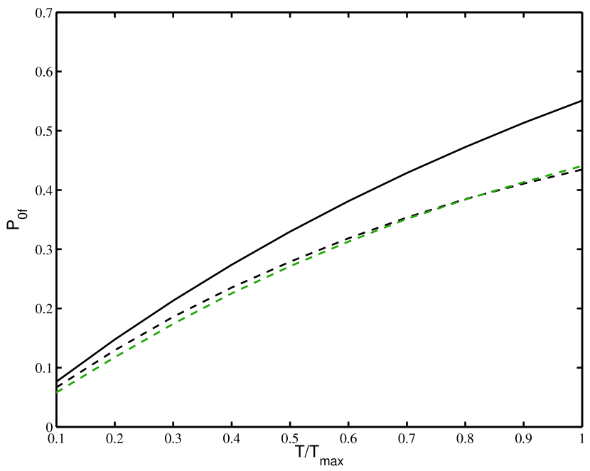
(a) Fig 1.a.

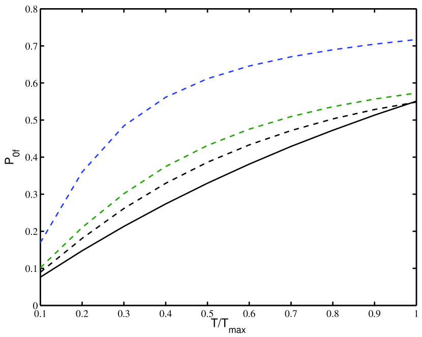
(b) Fig. 1.b.

Figure 1: Considering the coupling with a thermal environment, final success probability of the algorithm with adiabatic final adiabatic time $T$, as a function of $T/T_{\textmd{max}}$ (being $T_{\textmd{max}}=0.8T_{lin}$, with $T_{lin}=\frac{4N}{\pi}$, the time required for final success probability $0.55$ in the closed case) for different coupling parameters $\eta$, and for two cases: Fig 1.a. considering complex dissipation rates $\Gamma_{ij}$ (with $i,j=0,1$), as they appear naturally in the derived Bloch-Redfield equations, and Fig 1.b. considering only the real part of the dissipation rates $\Re\{\Gamma_{ij}\}$ (discontinuous lines). In both figures, the black solid line corresponds to the closed case $\eta=0$, while black, green and blue discontinuous lines corresponds to $\eta=0.05,0.1,0.5$ respectively. The curve $\eta=0.5$ is not shown in Fig 1.a., since for that value the imaginary part of the rates is too large and gives rise to unphysical results, what points out a failure of the weak coupling assumption. The frequency cut is chosen as $\omega_{c}=0.25$.

4.2 Structured environment

The effect of dissipation on the performance of the adiabatic search will depend on the details of the environment and its interaction with the system. The particular features of the adiabatic search make it specially sensitive to energy scales in the bath that are comparable to the characteristic gap in the system, $\Delta E$ [3, 10]. Intuitively, one would expect that the algorithm is more resilient when this energy corresponds to a gap in the spectral function of the environment (i.e. a frequency region where this function is zero), similar to the effect when the dominant energy scale of the bath is far away from $\Delta E$, as studied for the thermal case in [10]. However, while this picture gives a qualitative image, a complete idea of the effect of the environment in the algorithm can only be achieved with a more complete study. With this aim, in the following we analyse in detail the effect of an structured environment in the performance of the search algorithm. Particularly, we will consider an environment with a gap in the density of states (which leads to a gap in the spectral density), and which has the same characteristics as the radiation field within a photonic crystal. In addition to that, it is specially interesting to consider the case of a controllable environment, where the capability to tune the parameters of the interaction may give us the possibility to improve the performance of the algorithm via the dissipative dynamics. Such an environment is indeed realizable in the context of optical lattices, as we discuss in the following.

Let us therefore consider an ideal situation in which the quantum search algorithm is implemented in an atom lattice, which is formed by loading a gas of ultracold atoms in a standing wave field. In the last few years, atom lattices have been experimentally realized by several groups [22, 23, 24, 25, 26, 27], and due to their high controllability, they have also been proposed as a candidate to realize a quantum computer [27].

In addition, it has been recently shown [28, 16] that atoms in an optical lattice can be coupled to an environment in a controlled way. In the later proposal, atoms are considered to have two relevant internal states $a$ and $b$. Atoms in state $a$ are actually trapped by the optical lattice, and have a frequency $\omega_{a}=\omega_{a}^{0}+\omega_{0}/2$, with $\omega_{0}$ the trap frequency of the lattice. In addition, they are considered to be in the so-called strongly correlated regime, where either there is one or zero atoms at each site of the lattice. Atoms in state $b$ are not trapped by the lattice potential, and have an energy $\hbar\omega_{b}+\frac{\hbar k^{2}}{2m}$, where $\hbar\omega_{b}$ and $\frac{\hbar k^{2}}{2m}$ correspond to the internal and kinetic energies, respectively. If a Raman transition of total frequency $\omega_{L}$ and Rabi frequency $\Omega_{L}$ is produced between the trapped and the untrapped state, the Hamiltonian that describes this process can be written in the interaction picture as

$$H_{\textmd{int}} = \sum_{\bf j}\sum_{\bf k}g_{k}\left(b^{\dagger}_{\bf k}\sigma_{\bf j}e^{i\Delta_{\bf k}t-i({\bf k}-{\bf k}_{L})\cdot{\bf r}_{\bf j}}+h.c.\right).$$ (22)

In (22), the sum in $j$ runs over the $N$ sites in the lattice, ${\bf r}_{\bf j}$ denotes the positions in the lattice, and $\Delta_{\bf k}=k^{2}/2m-\Delta_{L}$, with $\Delta_{L}=\omega_{L}-(\omega_{b}-\omega_{a})$ the laser detuning. The coupling constants are $g_{k}=\Omega_{L}e^{-X_{0}^{2}k^{2}/2}(8\pi^{3/2}X_{0}^{3}/V)^{1/2}$, where $X_{0}=(1/2m\omega_{0})^{1/2}$ is the size of the wave function at each site.

The previous Hamiltonian is very similar to the one describing the interaction of two level atoms with the radiation field. However, here the spin operators $\sigma_{i}$ (equivalently $\sigma_{i}^{\dagger}$) are not describing transitions between atomic internal states, but rather they describe transitions from a Fock state $|1\rangle_{i}$ (which corresponds to the presence of an atom at site $i$), to the Fock state $|0\rangle_{i}$, describing the absence of atoms at site $i$. On the other hand, the operators $b^{\dagger}_{\bf k}$ (equivalently $b_{\bf k}$) correspond to the creation (annihilation) operators of a bath of harmonic oscillators, which in this case is not the radiation field, but the matter-wave field that describes the untrapped atoms.

In our model, we assume that the qubits undergoing adiabatic evolution are encoded in the presence $|1\rangle_{i}$ or absence $|0\rangle_{i}$ of an atom at site $i$ of the lattice. The coupling with the environment produces transitions between these basis states through the Hamiltonian (22). However, contrary to the case of the thermal environment studied in the former section, here the coupling with an environment is not an uncontrolled event, but rather it is artificially produced through the two-photon Raman transition to the untrapped level. For that reason, several external parameters that describe the interaction can be easily controlled: most importantly $\Omega_{L}$, which determines the coupling strength, $\Delta_{L}$, which determines the resonance condition, and $\omega_{0}$, which determines the trapping frequency of each lattice well, and as we will later see, will also characterize the width of the spectral function in the frequency space $J(\omega)$.

It is important to notice that, contrary to the thermal case, in this situation the correlation function can be fully determined by the coupling parameters $g_{k}$ and the dispersion relation of the environment, given by $\omega_{k}=\frac{k^{2}}{2m}+\omega_{b}$. No phenomenological model is needed to characterize the spectral function. On the other hand, the relation $\omega_{k}$ indeed resembles that of the radiation field in a three dimensional and infinite photonic crystal near the band-gap edge, which here corresponds to the frequency $\omega_{b}$ [29, 30, 31]. This environment will give rise to a very particular dissipation in our system. The correlation function can be written as [16]

$$g(t)=\sum_{\bf k}g_{k}^{2}e^{-i\Delta_{\bf k}t}=\Omega_{L}^{2}\frac{e^{i\Delta_{L}t}}{\nu_{t}^{3}},$$ (23)

where we have assumed that the sum in the wave vector $\bf{k}$ can be performed in the continuum limit. Here, the quantity $\nu_{t}=\sqrt{1+i\omega_{0}t}$.

In figure 2 we observe, always in the two-level approximation and for various parameter regimes, a larger final probability of success at small values of $T$ for the open system (discontinuous lines) than for the closed one (solid line). Similarly, figure 3 shows an improvement in the algorithm performance for certain values of $\Delta_{L}$. This results suggests that, at least within the two level approximation, a controlled coupling with a certain environment may improve the performance of the quantum search algorithm. Figures 2 and 3 show the result for the same parameter regimes as in 2 and 3 respectively, but just considering in the equations the real part of the dissipation rates. Just as in the case of the thermal environment, we can see that results for real and complex rates differ considerably.

Indeed, considering the full complex rates is particularly important for a structured environment like the one analysed here. When the system frequency is within the gap, the corresponding rate is, at long times, a purely imaginary quantity. Hence, by only considering the real part of the rates one would arrive to the wrong conclusion that the environment has no effect at all in the system. However, it has been known for a long time that even when the system resonant frequency is within a gap of the spectral density, the coupling with the environment has important consequences in its dynamics. Among other things, a so-called photon-atom bound state is formed [29], in which the energy is coherently interchanged between system and environment. This particular state, and more generally the dynamics of the system with a resonant frequency within the environment gap, can only be properly described when considering the imaginary part of the rates.

In addition we note that, while in the thermal case the improvement of the algorithm performance observed for real rates can no longer be observed when considering the full complex rates, the opposite is observed here. Indeed, as noted above only when complex rates are included in the description, an increase in the final success probability is observed for certain parameter regimes. This can be seen again by comparing figures 2 and 3, corresponding to real rates, with 2 and 3.

From all this we again conclude how crucial it is to consider the imaginary terms of the dissipation rates in order to correctly describe the system dynamics.

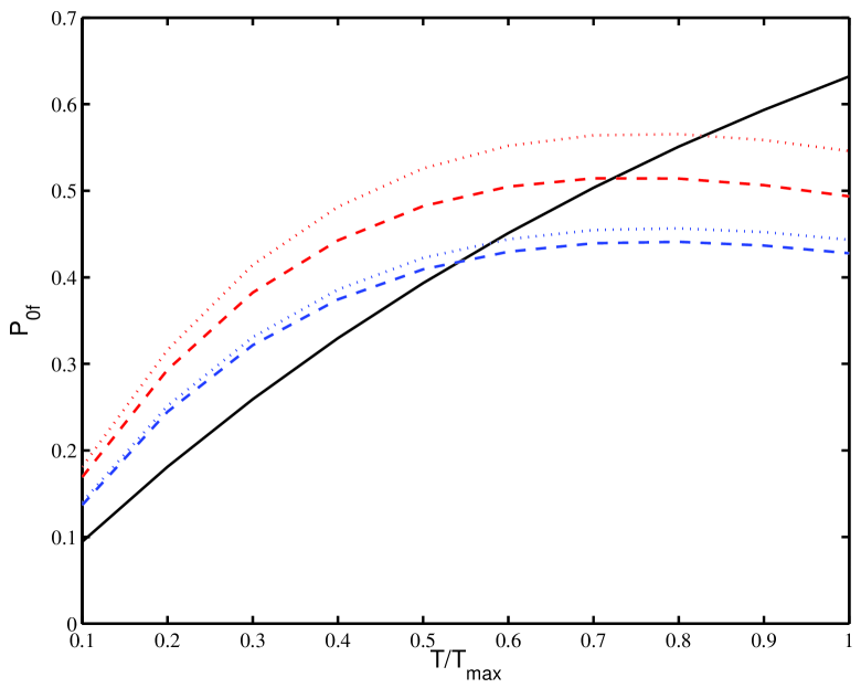
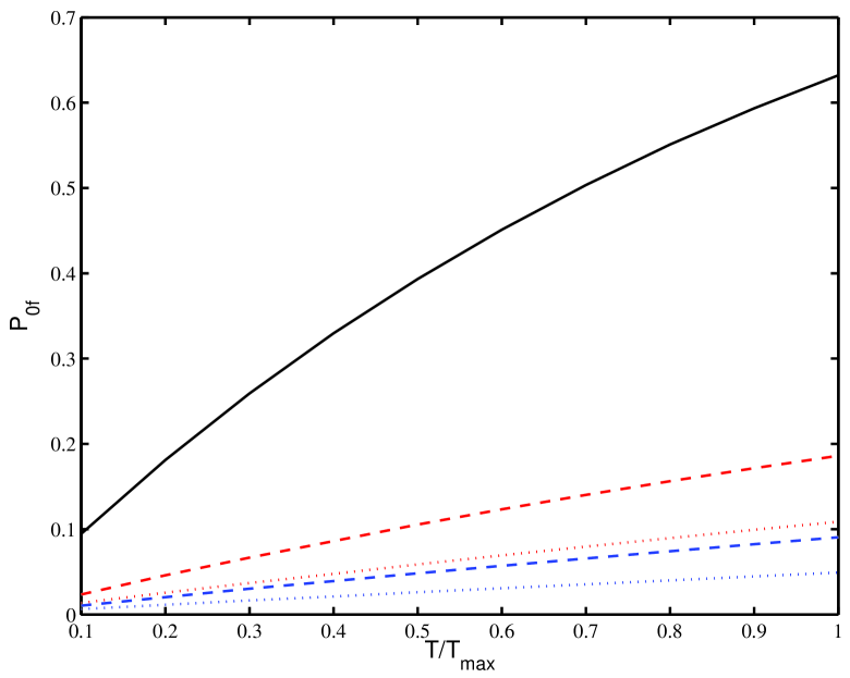
Figure 2: For a system coupled with a structured environment, the figures show the final success probability of the algorithm as a function of $T/T_{\textmd{max}}$ (with $T_{\textmd{max}}=T_{lin}$, and $T_{lin}=\frac{4N}{\pi}$). Solid black lines represent the solution for a closed system; red and blue dashed lines correspond to $\eta=0.05$ with $\Delta_{L}=0.2$ and $0.27$ respectively; red and blue dotted lines correspond to $\eta=0.1$ with $\Delta_{L}=0.2$ and $0.27$ respectively. Fig 1.a. represents the curves for complex rates, and for different couplings $\gamma$ and laser detunings $\Delta_{L}$. Fig 2.a. represents the curves for the same parameters but considering only the real part of the dissipation rates. In both cases the trap frequency is chosen as $\omega_{0}=0.25$.

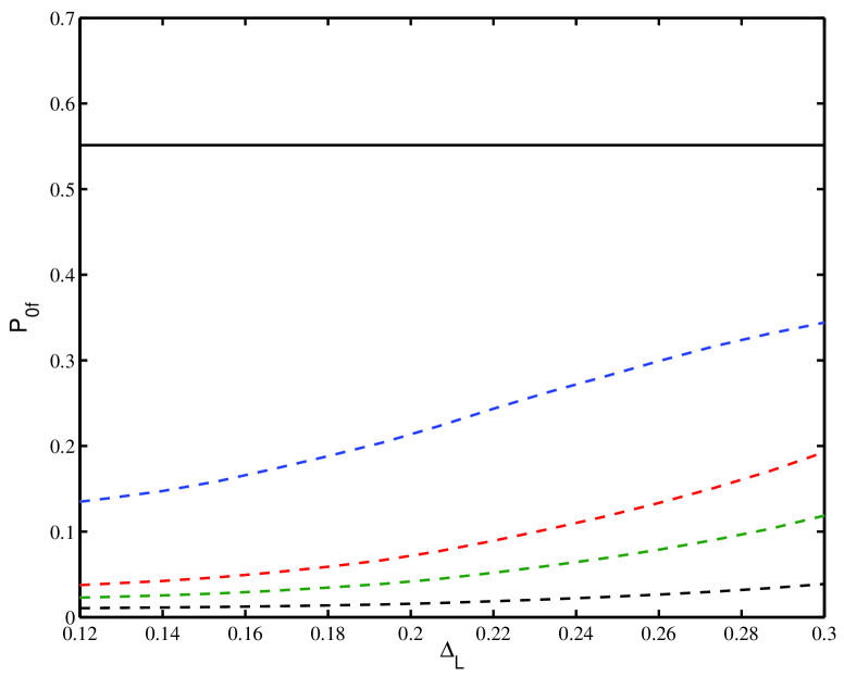
Figure 3: For a system coupled with a structured environment, the final success probability of the algorithm is plotted as a function of the laser detuning $\Delta_{L}$. Fig. 3.a represents the solutions considering complex rates. In this figure, the solid black line represents the solution for the closed system, while black, green, red and blue discontinuous lines correspond to couplings $\eta=0.01,0.05,0.1,0.4$ (from the bottom up) respectively. Fig. 3.b. shows the curves considering only the real part of the dissipation rates. In this figure, the solid black line represents the solution for the closed system, while black, green, blue discontinuous lines correspond to couplings $\eta=0.01,0.05,0.2$ (from the bottom up) respectively. The trap frequency is chosen as $\omega_{0}=0.25$, and $T_{max}=0.8\ T_{lin}$, with $T_{lin}=\frac{4N}{\pi}$.

4.3 Application to a genuine two-level system

In the former section we have seen within the two-level approximation, how an adiabatic search algorithm can be improved by connecting the system to a photonic crystal like environment as the one described in [16]. We are aware that the applicability of this result to a future implementation of the adiabatic version of the Grover’s algorithm depends on how good the two-level approximation is. The validity of the two-level approximation will be analyzed in more detail in Sect. 5. Notice, however, that this caveat would not apply to a genuine two-level system controllably coupled to a dissipative environment. Therefore in this section we will study if a real two level system undergoing a more general adiabatic evolution (not necessarily corresponding to the initial conditions of Grover’s algorithm) would also experience an improvement in the final result under some condition. We recall that here an improvement means that at the end of the adiabatic evolution, the population of the ground state of the final Hamiltonian is larger than in the closed system case.

To this order we consider the Hamiltonian (22) but with $n=1$, corresponding to a single site in the lattice. This model can be realized by considering a lattice with a filling factor sufficiently low so that the sparse atoms do not interact with each other. Hence, in a real setup we would have several independent copies of atoms at single sites. Instead of the adiabatic search algorithm, which should be realized with $N$ sites, let us consider an adiabatic process described by the Hamiltonian (4), but with $|m\rangle=|1\rangle$ and $|\psi_{0}\rangle=a_{0}|0\rangle+b_{0}|1\rangle$ with arbitrary coefficients $a_{0}$ and $b_{0}=\sqrt{1-a_{0}^{2}}$.

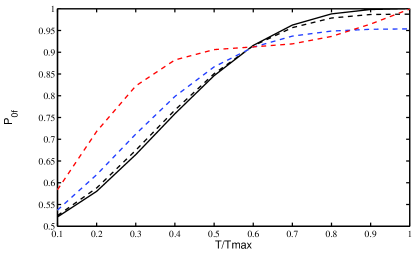
Figure 4: Final success probability (population of the ground state of the final Hamiltonian) for a genuine two level system undergoing adiabatic evolution, considering different adiabatic evolution times $T$, with $T_{\textmd{max}}=10$ (the approximate time in which the closed system reaches a success probability equal to one). The solid line corresponds to the closed system, while black, green and red discontinuous lines correspond to the results for $\eta=0.01,0.05,0.2$ respectively. Other parameters are chosen as $\omega_{0}=0.5$, $\Delta_{L}=0.5$, and $a_{0}=\sqrt{0.5}$.

We observe in Figure 4 that, for certain parameter regimes the final probability of success for the open system is larger than for the closed system. Similar results have been observed for other choices of the coefficient $a_{0}$. Hence, we conclude that the improvement of the adiabatic evolution for the system coupled with the environment is a robust effect in the two-level system, not linked to the particular choice of initial state in the search algorithm. Although in this section we have studied in particular a system subject to a photonic crystal-like environment, we believe that similar results could be encountered in other different scenarios, provided that the interaction between the system and the environment can be externally controlled. A simple example would be an atom in which the transition between the two relevant internal levels is produced by a two-photon process, mediated by a single laser followed by a spontaneous emission. This corresponds in quantum optics to a $\Lambda$ scheme, and would give rise to an effective Hamiltonian of the form (22). Despite having a different dispersion relation, this Hamiltonian would describe a coupling with the environment that can be tuned through the laser Rabi frequency.

5 Spectral density and the validity of the two level approximation

Let us now qualitatively study the validity of the two-level approximation. This approximation is suitable when the environment does not produce significant transitions to other levels of the energy spectrum different than $|0\rangle$ and $|1\rangle$, the ones involved in the quantum search algorithm. In general, the transition probability per unit time between two system levels $|i\rangle$ and $|j\rangle$ is approximately given by the Fermi Golden Rule as $P_{ij}\approx J(\omega_{ij})\langle i|H_{\textmd{int}}|j\rangle$. From this formula, we can already see that the spectral density, $J(\omega)$, is indeed a very important quantity that determines, at each frequency, what is the density of environmental states available, and how strong the coupling is. Indeed, one may expect that the two-level approximation applies better to parameter regimes such that the spectral density is small for frequencies corresponding to transitions to levels different from $|0\rangle$ and $|1\rangle$.

Notice that this can only be understood as a first qualitative approach to the question of the validity of this approximation. Firstly, because an equally important factor to determine $P_{ij}$ is the magnitude of the transition amplitudes $\langle i|H_{\textmd{int}}|j\rangle$, and secondly, because $P_{ij}$ only accounts for the real part of the transition rates.

Let us illustrate this qualitative approach by considering the energy vs. time plot in figure 5 for the thermal bath. All energy differences $E_{i}-E_{j}$ in the closed system are represented in the plot as solid lines. The background shows how the spectral density varies for different energies, with darker color representing a larger value of $J$. Intuitively we expect that a particular transition $i\rightarrow j$ becomes more important when the corresponding energy gap coincides with large values of $J(\omega)$.

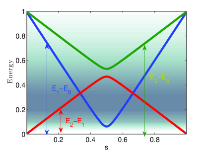
Figure 5: The energy gaps in the closed system as a function of the adiabatic parameter $s$: $E_{1}-E_{0}$ (blue), $E_{2}-E_{1}$ (red) and $E_{2}-E_{0}$ (green). For each value of energy, the background color indicates the magnitude of the spectral density for a thermal bath, where we have chosen the same parameters as in section (4.1), $s=1$ and $\omega_{c}=0.25$.

In order to compute the spectral function for the photonic crystal-like environment, let us consider the calculus of the correlation function of the system as defined in (23),

$$g(t)=\frac{4\pi\Omega_{L}^{2}X_{0}^{3}}{\pi^{3/2}}\int_{0}^{\infty}dkk^{2}e^{-i(\frac{k^{2}}{2m}-\Delta_{L})t}e^{-{X_{0}^{2}k^{2}}}.$$ (24)

Here, both $g_{k}$ and $\omega_{\bf k}$ only depend on the modulus of the wave vector. Using this, the angular part of the integral has been performed (giving rise to a factor $4\pi$) and only the integral of the modulus is left. We can consider that the coupling parameter $g_{\bf k}$ does only depend on the modulus of the wave vector, because it has been assumed that the total wave vector of the Raman lasers ${\bf k}_{L}\approx 0$. According to the definition (20), the spectral function is the kernel of the integral (24) translated to the frequency space. Hence, it is necessary to use the dispersion relation $\omega(k)=\frac{k^{2}}{2m}+\omega_{b}$ in order to perform a change of variable in the integral (24), such that it becomes an integral in $\omega$,

$$g(t)=\eta\int_{\omega_{b}}^{\infty}d\omega\sqrt{2(\omega-\omega_{b})}e^{-i(\omega-\omega_{L})t}e^{-2\frac{\omega-\omega_{b}}{\omega_{0}}},$$ (25)

with $\eta=\frac{8\pi^{1/2}\Omega_{L}^{2}}{\omega_{0}^{3/2}}$. Considering now an energy shift of the form $\hat{\omega}=\omega-\omega_{L}$, the former integral is just

$$g(t)=\eta\int_{\Delta_{L}}^{\infty}d\omega\sqrt{2(\omega-\Delta_{L})}e^{-i\omega t}e^{-2\frac{\omega-\Delta_{L}}{\omega_{0}}}.$$ (26)

Since in this case the temperature of the reservoir is zero, it is straightforward to see that the spectral density has the form $J(\omega)=\eta\sqrt{2(\omega-\Delta_{L})}e^{-2\frac{\omega-\Delta_{L}}{\omega_{0}}}$.

Like in the thermal case, figure 6 represents all energy differences $E_{i}-E_{j}$ for the closed system in solid lines, compared to the spectral density in the background. From a naive interpretation of the picture, one would consider that, since the minimum gap $E_{1}-E_{0}$ corresponds to an energy within the environment gap, where the spectral density is zero, the effects of the environment are somehow minimized. However, as it is shown in figure  2, for the same $\Delta_{L}=0.28$, the performance of the algorithm is even improved with respect to that of the closed system. Hence, the environment gap does not protect the algorithm from the interaction, but rather it produces some positive effects on its performance.

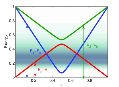
Figure 6: The energy gaps in the closed system as a function of the adiabatic parameter $s$: $E_{1}-E_{0}$ (blue), $E_{2}-E_{1}$ (red) and $E_{2}-E_{0}$ (green). The background indicates the magnitude of the spectral density for the photonic crystal-like environment, with $\Delta_{L}=0.28$ and $\omega_{0}=0.25$ as typical parameters used in section (4.2). We expect that the dominant transitions induced by the couplig to the environment are $0\leftrightarrow 1$. The transition $1\leftrightarrow 2$ may also contribute, but it will be suppressed during the first part of the algorithm because the $E_{1}$ level is initially not populated. It will again be important after $s\approx 0.65$. With these parameters, moreover, the minimum gap, around $s=0.5$, is decoupled from the frequencies of the bath, what can be expected to bring some protection to the most sensitive part of the algorithm.

As already mentioned, another important factor that determines the transition probability to other levels $|i\rangle$ different to the ones considered in the two level approximation ($|0\rangle$ and $|1\rangle$) is the amplitude of the transition elements $\langle i|H_{\textmd{int}}|0\rangle$, $\langle i|H_{\textmd{int}}|1\rangle$, and in general $\langle i|H_{\textmd{int}}|j\rangle$, with $H_{\textmd{int}}$ given by (22). However, this analysis is out of the scope of the present paper, and will be made elsewere.

6 Conclusions

We have studied the performance of the adiabatic quantum search in a dissipative environment. Our derivation of the Bloch-Redfield equation allows for a more complete account of the effects of the complex dissipation rates than previous studies. In particular, we have shown that neglecting the imaginary parts of such rates give rise to a completely different dynamic than when considering the full complex rates. Hence, conclusions about whether there is an improvement of the performance of the adiabatic algorithm within an open system, cannot be extracted by a partial analysis that only accounts for the real part of the dissipation rates.

Particularly, we have analyzed the effect of the dissipation on the adiabatic version of Grover’s algorithm for two different settings, namely a thermal bath and a controllable environment with tunable parameters. While for a thermal environment no improvement is observed in the performance of the algorithm, coupling the system to a structured environment gives rise to a final success probability that for certain parameter regimes is higher than in the closed system case. Hence, we have found an example in which the performance of the search can be improved with respect to the closed system, by tuning the bath parameters appropriately.

Our study, valid for the quantum search in the framework of the two-level approximation, can be extended to the adiabatic evolution of a genuine two-dimensional system.

We acknowledge J. I. Cirac, S. F. Huelga, M. B. Plenio for support, and A. M. S. Amin for interesting discussions. We also thank ’Centro de ciencias de Benasque’ for its hospitality. This work has been supported in part by the Spanish Ministerio de Educación y Ciencia through Projects AYA2007-67626-C03-01 and FPA2008-03373, by the ’Generalitat Valenciana’ grant PROMETEO/2009/128, by the DFG Cluster of Excellence MAP, the SFB 631, and the DFG Forschergruppe 635, and by the EU (FP7/2007-2013) under grant agreement nr. 247687 (Integrating Project AQUTE).

7 Appendix A

In this appendix we proceed to derive equation (10) in the paper. The total density matrix can be written in the form

$$\rho_{\textmd{tot}}(t)=\rho_{S}(t)\otimes\rho_{B}(t)+\rho_{\textmd{correl}},$$ (27)

where $\rho_{S}=Tr_{B}(\rho_{\textmd{tot}}(t))$ and $\rho_{B}=Tr_{S}(\rho_{\textmd{tot}}(t))$ are the reduced density matrices of the system and the bath, respectively, and $\rho_{\textmd{correl}}$ describes the correlations existing between system and environment. We assume that in general we are dealing with a thermal bath, so that $\rho_{B}=e^{-\beta H_{B}}$, with $\beta=1/(K_{B}T)$, $K_{B}$ the Boltzmann constant and $T$ the temperature of the reservoir. We consider the master equation for the reduced density operator in the interaction picture with respect to both the system and the environment, $\rho_{SI}={\mathcal{U}}^{\dagger}(t)\rho_{S}{\mathcal{U}}(t)$, where $\mathcal{U}(t)$ is given by the time-ordered exponential ${\mathcal{U}}(t)=Te^{-i\int_{0}^{t}H_{S}(\tau))d\tau}$. Considering that $\frac{d{\mathcal{U}}^{\dagger}(t)}{dt}=iH_{S}(t){\mathcal{U}}^{\dagger}(t)$, the evolution equation up to second order in $g=\|H_{\textmd{int}}\|/\|H_{S}+H_{B}\|$ is given by [32]

$$\dot{\rho}_{SI}(t)=-\int_{0}^{t}d\tau Tr_{B}[H_{I}(t),[H_{I}(\tau),\rho_{SI}(t)\otimes\rho_{B}]].$$ (28)

Here the terms $\sim Tr_{B}(\rho_{B}H_{\textmd{int}}^{t})$ have been neglected, an assumption that is valid for most types of environments and couplings. Particularly, it is valid for our present case of a system lineraly coupled to an environment of harmonic oscillators. In addition, it has also been assumed that $\rho(t)=\rho_{S}(t)\otimes\rho_{B}$, and since $\tau_{C}\ll 1/\Gamma$, we have also assumed that $\rho_{SI}(\tau)\approx\rho_{SI}(t)$ in the integral. On the other hand, the quantity $H_{I}(t)={\mathcal{U}}^{\dagger}(t)H^{t}_{\textmd{int}}{\mathcal{U}}(t)$ with $H^{t}_{\textmd{int}}=e^{iH_{B}t}H_{\textmd{int}}e^{-iH_{B}t}$. Going back to the original picture, the evolution equation of $\rho_{S}$ is then given by

$$\frac{d\rho_{S}}{dt} = -i[H_{S}(t),\rho_{S}]$$ (29)

$$- \int_{0}^{t}d\tau{\mathcal{U}}(t)Tr_{B}[H_{I}(t),[H_{I}(\tau),\rho_{SI}(t)\otimes\rho_{B}]]{\mathcal{U}}^{\dagger}(t).$$

The latter equation can also be expressed as

$$\frac{d\rho_{S}}{dt}=-i[H_{S}(t),\rho_{S}]-\int_{0}^{t}d\tau Tr_{B}\left[H^{t}_{\textmd{int}},[H_{I}(\tau,-t),\rho_{S}(t)\otimes\rho_{B}]\right],$$ (30)

where $H_{I}(\tau,-t)={\mathcal{U}}(t){\mathcal{U}}^{\dagger}(\tau)H^{\tau}_{\textmd{int}}{\mathcal{U}}(\tau){\mathcal{U}}^{\dagger}(t)$. Expanding the commutator on the right hand side of the last equation, we find the following terms,

$$Tr_{B} \left([H^{t}_{\textmd{int}},[H_{I}(\tau,-t),\rho_{S}(t)\rho_{B}]]\right)=Tr_{B}\big{(}\{H^{t}_{\textmd{int}}H_{I}(\tau,-t),\rho_{S}\otimes\rho_{B}\}$$ (31)

$$- H^{t}_{\textmd{int}}\rho_{S}\otimes\rho_{B}H_{I}(\tau,-t)-H_{I}(\tau,-t)\rho_{S}\otimes\rho_{B}H^{t}_{\textmd{int}}\big{)}.$$

Let us now consider our case, in which the interaction Hamiltonian can be written as $H_{\textmd{int}}=A\otimes B$, where $A=\sigma_{z}$ and $B=\sum_{\lambda}g_{\lambda}(b_{\lambda}^{\dagger}+b_{\lambda})$. We can make further simplifications in equation (31)

$$Tr_{B} \left([H^{t}_{\textmd{int}},[H_{I}(\tau,-t),\rho_{S}(t)\otimes\rho_{B}]]\right)$$ (32)

$$= g(t-\tau)\left(AA(\tau,-t)\rho_{S}-A(\tau,-t)\rho_{S}A\right)$$

$$+ g(\tau-t)\left(\rho_{S}A(\tau,-t)A-A\rho_{S}A(\tau,-t)\right),$$

where $A(\tau-t)={\mathcal{U}}(t){\mathcal{U}}^{\dagger}(\tau)A{\mathcal{U}}(\tau){\mathcal{U}}^{\dagger}(t)$, and $g(t-\tau)=Tr_{B}[B^{t}B^{\tau}\rho_{B}]$, $g(\tau-t)=Tr_{B}[B^{\tau}B^{t}\rho_{B}]$, having the form

$$g(t)=\sum_{\lambda}g_{\lambda}^{2}[\coth{\left(\frac{\beta\omega_{\lambda}}{2}\right)}\cos{(\omega_{\lambda}t)}-i\sin{(\omega_{\lambda}t)}].$$ (33)

Here, we have taken into account that, for a thermal bath,

$$Tr_{B}(\rho_{B}b_{\lambda}^{\dagger}b_{\lambda^{\prime}})=\delta_{\lambda,\lambda^{\prime}}N(\omega_{\lambda}),$$

$$Tr_{B}(\rho_{B}b_{\lambda}b^{\dagger}_{\lambda^{\prime}})=1+\delta_{\lambda,\lambda^{\prime}}N(\omega_{\lambda}),$$ (34)

with $N(\omega_{\lambda})=1/(e^{\omega_{\lambda}\beta}-1)$ the number of excitations with frequency $\omega_{\lambda}$. Note that according to equation (11), $g(-t)=g^{*}(t)$. Considering that, and inserting (32) in (30) we find

$$\frac{d\rho_{S}}{dt} = -i[H_{S}(t),\rho_{S}]-\int_{0}^{t}d\tau g(t-\tau)\left(AA(\tau,-t)\rho_{S}-A(\tau,-t)\rho_{S}A\right)$$ (35)

$$- \int_{0}^{t}d\tau g^{*}(t-\tau)\left(\rho_{S}A(\tau,-t)A-A\rho_{S}A(\tau,-t)\right).$$

References

- [1] Edward Farhi, Jeffrey Goldstone, Sam Gutmann, and Michael Sipser. Quantum computation by adiabatic evolution, 2000. arXiv:quant-ph/0001106v1.
- [2] D. Aharonov, W. van Dam, J. Kempe, Z. Landau, S. Lloyd, and O. Regev. Adiabatic quantum computation is equivalent to standard quantum computation. Annual IEEE Symposium on Foundations of Computer Science, pages 42–51, 2004.
- [3] A. M. Childs, E. Farhi, and J. Preskill. Robustness of adiabatic quantum computation. Phys. Rev. A, 65(1):012322, Dec 2001.
- [4] M. Born and V. Fock. Beweis des adiabatensatzes. Zeitschrift fur Physik, 51:165–180, March 1928.
- [5] T. Kato. On the adiabatic theorem of quantum mechanics. Journal of the Physical Society of Japan, 5:435, November 1950.
- [6] Albert Messiah. Quantum Mechanics, chapter xvii. Dover Publications, 1999.
- [7] A. Ambainis and O. Regev. An elementary proof of the quantum adiabatic theorem. quant-ph/0411152, pages 1–12, 2004.
- [8] D. A. Lidar, A. T. Rezakhani, and A. Hamma. Adiabatic approximation with exponential accuracy for many-body systems and quantum computation. J. Math. Phys, 50:102106, 2009.
- [9] M.S. Sarandy and D.A. Lidar. Adiabatic approximation in open quantum systems. Phys. Rev. Lett., 95(25):250503, 2005.
- [10] M. H. S. Amin, Peter J. Love, and C. J. S. Truncik. Thermally assisted adiabatic quantum computation. Phys. Rev. Lett., 100(6):060503, Feb 2008.
- [11] M. H. S. Amin, Peter J. Love, and C. J. S. Truncik. Role of single-qubit decoherence time in adiabatic quantum computation. Phys. Rev. A, 80(2):022303, Aug 2009.
- [12] L. K. Grover. Quantum mechanics helps in searching for a needle in a haystack. Phys. Rev. Lett., 79:325, 1997.
- [13] J. Roland and N. J. Cerf. Quantum search by local adiabatic evolution. Phys. Rev. A, 65(4):042308, Mar 2002.
- [14] Markus Tiersch and Ralf Schützhold. Non-markovian decoherence in the adiabatic quantum search algorithm. Phys. Rev. A, 75(6):062313, Jun 2007.
- [15] A J Leggett, S Chakravarty, A. T Dorsey, Anupam Fisher, Matthew P. A. Garg, and W. Zwerger. Dynamics of a dissipative two-state system. Rev. Mod. Phys, 59(6):1, Jun 1987.
- [16] I. de Vega, D. Porras, and I. Cirac. Matter-wave emission in optical lattices: Single particle and collective effects. Phys. Rev. Lett., 101(6):260404, Jun 2008.
- [17] Charles H. Bennett, Ethan Bernstein, Gilles Brassard, and Umesh Vazirani. Strengths and weaknesses of quantum computing. SIAM Journal on Computing, 26(5):1510–1523, 1997.
- [18] C. Zalka. Grover’s quantum searching algorithm is optimal. Phys. Rev. A, 60:2746, 1999.
- [19] A. Pérez. Hilbert-space average method and adiabatic quantum search. Phys. Rev. A, 79(1):012314, 2009.
- [20] Ali Mostafazadeh. Quantum adiabatic approximation and the geometric phase. Phys. Rev. A, 55(3):1653–1664, Mar 1997.
- [21] M.O. Scully and M. Suhail Zubairy. Quantum Optics. Oxford Univ. Press, 2002.
- [22] D. Jaksch, C. Bruder, J. I. Cirac, C. W. Gardiner, and P. Zoller. Cold bosonic atoms in optical lattices. Phys. Rev. Lett., 81(15):3108–3111, Oct 1998.
- [23] O. Mandel, M. Greiner, A. Widera, T. Rom, T. W. Hänsch, and I. Bloch. Controlled collisions for multi-particle entanglement of optically trapped atoms. Nature, 425:937, 2003.
- [24] M. Greiner, O. Mandel, T. Esslinger, T. W. Hänsch, and I. Bloch. Quantum phase transition from a superfluid to a mott insulator in a gas of ultracold atoms. Nature, 415:39, 2002.
- [25] S. Fölling, F. Gerbier, A. Widera, O. Mandel, T. Gericke, and I. Bloch. Spatial quantum noise interferometry in expanding ultracold atom clouds. Nature, 434:481–484, 2005.
- [26] B. Paredes, A. Widera, V. Murg, O. Mandel, S. Fölling, I. Cirac, G. V. Shlyapnikov, T. W. Hänsch, and I. Bloch. Tonks–girardeau gas of ultracold atoms in an optical lattice. Nature, 424:277, 2004.
- [27] Immanuel Bloch, Jean Dalibard, and Wilhelm Zwerger. Many-body physics with ultracold gases. Rev. Mod. Phys., 80(3):885–964, 2008.
- [28] A. Recati, P. O. Fedichev, W. Zwerger, J. von Delft, and P. Zoller. Atomic quantum dots coupled to a reservoir of a superfluid bose-einstein condensate. Phys. Rev. Lett., 94(4):040404, 2005.
- [29] M. Woldeyohannes and S. John. Coherent control of spontaneous emission near a photonic band edge. Journal of Optics B: Quantum and Semiclassical Optics, 5(2):R43–R82, 2003.
- [30] S. John and T. Quang. Localization of superradiance near a photonic band gap. Phys. Rev. Lett., 74(17):3419–3422, 1995.
- [31] Inés de Vega, Daniel Alonso, and Pierre Gaspard. Two-level system immersed in a photonic band-gap material: A non-markovian stochastic schrödinger-equation approach. Phys. Rev. A, 71(2):023812, 2005.
- [32] M. H. S. Amin. Bloch-redfield formalism for qubits. Unpublished notes (private communication).