Strain in Semiconductor Core-Shell Nanowires
Abstract
We compute strain distributions in core-shell nanowires of zinc blende structure. We use both continuum elasticity theory and an atomistic model, and consider both finite and infinite wires. The atomistic valence force-field (VFF) model has only few assumptions. But it is less computationally efficient than the finite-element (FEM) continuum elasticity model. The generic properties of the strain distributions in core-shell nanowires obtained based on the two models agree well. This agreement indicates that although the calculations based on the VFF model are computationally feasible in many cases, the continuum elasticity theory suffices to describe the strain distributions in large core-shell nanowire structures. We find that the obtained strain distributions for infinite wires are excellent approximations to the strain distributions in finite wires, except in the regions close to the ends. Thus, our most computationally efficient model, the finite-element continuum elasticity model developed for infinite wires, is sufficient, unless edge effects are important. We give a comprehensive discussion of strain profiles. We find that the hydrostatic strain in the core is dominated by the axial strain-component, . We also find that although the individual strain components have a complex structure, the hydrostatic strain shows a much simpler structure. All in-plane strain components are of similar magnitude. The non-planar off-diagonal strain-components ( and ) are small but nonvanishing. Thus the material is not only stretched and compressed but also warped. The models used can be extended for study of wurtzite nanowire structures, as well as nanowires with multiple shells.
pacs:
62.23.Hj, 62.35.-g, 62.20.D-, 68.70.+wI Introduction
Nanowires represent a promising technological platform with a wide range of applications spanning from electronic Huang et al. (2001) and photonic devicesLaw et al. (2005); Wang et al. (2008); Huang et al. (2005) to biochemical sensorsZheng et al. (2005). The reasons for this success are not only the increasing ability in handling and manipulating nanowires but also an ongoing improvement of the quality of the crystal structure of the grown wires.
The progress in crystal growth has led to the fabrication of coherent crystalline nanowires with core-shell structureLauhon et al. (2002). The differences between the materials of the core and shell in lattice constants and band parameters allow for tuning the properties of the resulting wire Skold et al. (2005). Possible strategies involve confining charge carriers to the nanowire core to reduce the influence of the surface on the electrical properties. Likewise, a core-shell nanowire can serve as an optical waveguide confining light. Confining charge carriers to the shell, or having multiple active shells and confining electrons and holes to different shells Schrier et al. (2007); Zhang et al. (2007), may also be relevant, depending on applications. The confinement can be obtained by band gap engineering and strain-engineering Boxberg and Tulkki (2007). In strain-engineering, one chooses to grow the core and shell in a nanowire with different materials with a coherent crystalline core-shell interface. Thus the nanowire is under a pseudomorphic strain, due to the deformations at the interface to accommodate the different lattice constants. This strain generates different deformation potentials in the core and shell regions which affect the electronic structure and thus the electrical and optical properties of the nanowires. In particular, gaining deep insight into the electronic structure of heterostructured nanowires with a lattice mismatch, requires finding the underlying elastic deformation, since this elastic information is needed as input to, e.g., or tight-binding calculations.Csontos et al. (2008, 2009); Persson and Xu (2002, 2004a, 2004b, 2006a, 2006b)
Theoretical investigations based on the continuum elasticity of systems experiencing pseudomorphic strain go back to Eshelby Eshelby (1957) who used analytical methods to study the strain effects of one material immersed in another. More recently, several studies of pseudomorphic strain fields have been performed for finite nanostructures.Stangl et al. (2004) On core-shell nanowire geometries, Niquet studied the effect of a shell on the electronic properties of a quantum dot embedded in a wire.Niquet (2006, 2007) Studies on the effect of a core-shell geometry on the electronic properties in quantum wires were also performed by Pistol and Pryor, Pistol and Pryor (2008) Schrier et al,Schrier et al. (2007) and Zhang et al.Zhang et al. (2007) However, these studies only considered very small structures or presented the hydrostatic strain in the structures.
In this article, we calculate and discuss the elastic deformation in core-shell nanowires of zinc blende structure with a lattice mismatch between the core and shell materials. Numerical calculations are performed for both finite and infinite wires using both continuum elasticity theory (implemented by a finite element scheme) and the atomistic model of Keating Keating (1966a). We present the strain distributions in a cross section of the nanowire as well as line scans both in the cross-section and along the wire. We consider free nanowires, i.e., we neglect external forces acting on the nanowires. Core-shell nanowires with various cross sections are investigated: hexagonal cross sections with both parallel and non-parallel core and shell facets and co-centric circular cross sections. We restrict ourselves to only discussing nanowires with a single shell and a core, although the methodology used here can be generalized to multiple shell nanowires. Likewise, we shall only consider purely zinc blende crystalline heterostructures.
II Continuum elasticity theory
We here describe the continuum elasticity (CE) model employed for a core-shell nanowire of zinc blende structure with axis along the direction for which the material lattice parameters vary discontinuously at the core-shell interface.
II.1 Coordinate systems
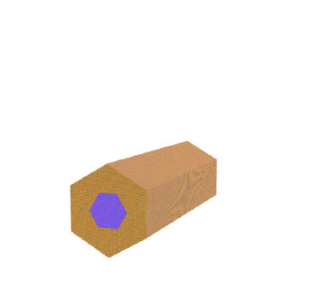
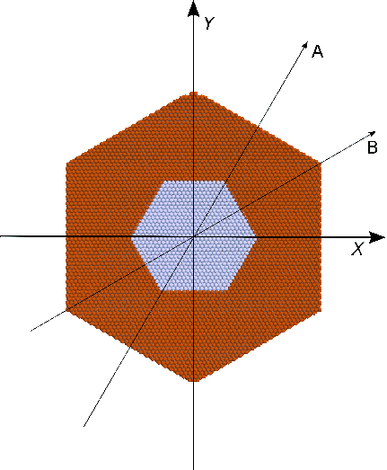
We consider core-shell nanowires of zinc blende structure with axis along the -direction. Figure 1 shows a typical core-shell nanowire geometry. We define two coordinate systems: a standard coordinate system with axes denoted by coinciding with the main crystallographic axes and another system where the axes will be denoted by , referred to as the nanowire-oriented coordinate system. In the system, the axis is parallel to the axis direction of the nanowire (i.e., the direction). The and axes are in the and crystal directions, respectively, as depicted in Fig. 2. Formally, the nanowire oriented coordinate system is related to the standard coordinate system by the transformation
| (1) |
with a rotation matrix given by
| (2) |
II.2 Strain energy
The strain energy is written as
| (3) |
where is the strain energy density, are the elastic stiffness tensor elements, and are strain tensor components Nye (1985).
For a material with cubic symmetry, the elastic stiffness tensor, , only has three independent elements and the strain energy density in the crystallographic coordinate system can be written as
| (4) |
where
| (5) |
The identities in Eq. (II.2) reflect the cubic symmetry of the material and define the general symmetry properties of the elasticity tensor.Nye (1985) In our calculations, numerical values of the are taken from Ref. Vurgaftman et al., 2001.
II.3 Incorporating pseudomorphic strain
In this section we describe the lattice matching conditions and their interpretation in two- and three-dimensional bulk systems.
II.3.1 Pseudomorphic conditions
We consider two different elastic media, which are the core and the shell materials of the same crystal structure. We shall use superscripts and to indicate core and shell, respectively. A typical geometry for a finite wire is shown in Fig. 1, and a cross section of the wire is shown in Fig. 2.
For cubic materials the lattice vectors and of core and shell in the strain-free state can be written as
| (6) |
where and are the lattice constants of the core and shell materials, and are the components of the lattice vectors in the core and shell, are integers, and are the basic vector in the crystallographic coordinate system.
After lattice deformation, distorted lattice vectors in the core and shell can be written in terms of the components and of the corresponding strain tensor, as
| (7) |
At the core-shell interface, the in-plane component of the distorted vector on the core side must match its equivalent on the shell side. This pseudomorphic requirement can be expressed as
| (8) |
where are the components of an arbitrary tangent vector of the interface. One implication of Eq. (8) is that the strain will be discontinuous at an interface between two cubic materials having different lattice constants.
II.3.2 Initial strain
To fulfill the conditions of Eq. (8), we assume the strain tensor in Eq. (3) is given by a sum of two terms
| (9) |
where is the displacement field relative to a matched (yet unrelaxed) configuration and is an initial strainPovolotskyi and Carlo (2006).
The initial strain is assumed nonvanishing only in the shell, where it is defined, in the cubic case, by
| (10) |
where and are the lengths of the lattice vectors in the core and the shell, respectively. This initial strain ensures that the conditions Eq. (8) are satisfied and leads to a matched structure.
The structure obtained for is not that of lowest energy for and the structure is relaxed by varying the field to minimize the energy Eq. (3). For a finite wire, the degrees of freedom to vary are precisely the degrees of freedom of . For the case of an infinite wire, the periodicity in the -direction is utilized and the resulting model is described below.
II.4 Infinite Wire
The model of an infinite wire utilizes the periodicity in the -direction and reduces the modeling domain to a 2-dimensional domain.
The strain tensor is transformed to the nanowire oriented coordinate system by
| (11) |
where Greek indices vary over and and Latin indices vary over and .
In the model of an infinite wire, the vectorial field introduced in Eq. (9) depends only on the coordinates in an plane of the nanowire, and we write . The axial strain in the core and the axial strain in the shell are constant and by Eq. (8) fulfill
| (12) |
The axial strain can thus be described as a single degree of freedom as
| (13) |
In the model of an infinite wire, the field and the variable are the degrees of freedom.
In this model, we keep and in contrast to the conventional plane strain approximation in which is assumedCleland (2003); Søndergaard et al. (2009).
The minimization of the strain energy over the variable corresponds to the condition that the total axial force vanishes. This has been discussed for a simpler energy functional in Ref. Søndergaard et al., 2009. The vanishing of the total axial force can be understood by considering a wire of a fixed number of unit cells . By translation invariance the total energy is proportional to . The variation of the energy per unit cell becomes
where and are the strain energies of core and shell. The energy is given by Eq. (3) with the integration taken over the undeformed domains Povolotskyi and Carlo (2006). For the core the undeformed axial length is proportional to and for the shell the axial length is proportional to . In particular, the total energy of the core with energy density is given by
| (17) |
For the variation of the core energy, we calculate the partial derivative
| (18) |
where is the axial stress. The area element and the axial stress then correspond to an infinitesimal axial force . Using these results and those similar for the shell, we can write
proving the assertion. This result [Eq. (II.4)] could be generalized to infinite wires under stretch. In that case we would use a non-zero force condition.
The actual minimization is done using finite elements Zienkiewicz and Taylor (1989) (linear triangular elements) for the continuous displacement and a variable to parameterize the axial strain [Eq. (13)]. The finite element method (FEM) is chosen due to its flexibility with respect to arbitrary geometries. The method leads to a sparse matrix problem of the form from which (representing and ) is solved by standard numerical packages. Note that here the variable couples to all other degrees of freedom in the matrix . This is unlike the usual setting of only local coupling in two- and three dimensional bulk structures. Still, in practice the solution is very fast even for meshes with around 30000 nodes and three degrees of freedom per node.
II.5 Finite Wire
We also compute the strain in finite core-shell nanowires. The strain is computed by minimizing the total strain energy, defined in Eq. 3. This is performed in the coordinate system , , and of the principal axes of the underlying crystal and by incorporating the pseudomorphic strain as described in Sec. II.3. For finite wires we have no benefit of using the nanowire oriented coordinate system because of the lack of translational symmetry.
The typical length of a modeled finite wire range from nm to nm. In the modeling of finite wires we exploit the symmetry of the nanowire. That is, we model and mesh only a segment of of the total nanowire geometry. On the nodes on the side facets of this segment we then fix the displacement perpendicular to the facetfootFBSymm . By this symmetry reduction we reduce the computational domain and the number of nodes by a factor of . This technique also reduce the source of numerical errors since the resulting element mesh has the same symmetry as the nanowire geometry.
The CE model of finite wires is implemented using three-dimensional tetrahedron elements with second order polynomials. A typical element mesh contain in total around nodes distributed in a wire, with 3 degrees of freedom per node. We use a nonuniform and adapted element mesh with at most nodes per cross-sectional area (on of the nanowire cross-section).
III Atomistic VFF Model
For the atomistic calculations we use the Valence-Force Field (VFF) model of KeatingKeating (1966a). The structure is built up one atomic layer at a time. We choose a layer structure that corresponds to a zinc blende phase nanowire with axis along the direction.
We first describe our model for finite wires and then describe our implementation for an infinite wire using translation invariance.
III.1 Finite wires
The atomic coordinates are the degrees of freedom of our VFF model. The energy is a function of these and is written as sums over interatomic bond distances and three-body bond angles.
We let denote the vector from atom to atom and denote the value takes in a stress-free bulk crystal. The potential energy of the crystal is given by Keating (1966a)
where the equilibrium bond angles fulfill in zinc blende and n.n. on top of a summation sign indicates that we sum over nearest neighbors of atom only.
Numerical values for the coupling constants and are obtained by comparing the energy in the VFF model Eq. (III.1) and the CE model Eq. (3), and requiring that the energies coincide for small deformations of a small volume. This requires three equations to be satisfied, one for each material parameter in the CE model. As the VFF model only contains the two coupling constants and , all three equations cannot be exactly satisfied, but any choice of values for and will give rise to effective elastic constants of the VFF model that deviate form the experimentally determined values used in the CE model. We follow Pryor et. al. Pryor et al. (1998) in using the values provided by Martin Martin (1970). Numerical values for the coupling constants and the relative errors in effective elastic constants are summarized in Tab. 1.
| GaAs | GaP | |
|---|---|---|
| () | 41.19 | 47.32 |
| () | 8.95 | 10.44 |
| (Å) | 2.448 | 2.36 |
| (%) | -0.22 | 2.7 |
| (%) | 1.7 | 9.1 |
| (%) | -13 | -11 |
Possible extensions of our model include an additional Coulomb interaction energy Martin (1970) and higher order terms for non-linear elasticity Keating (1966b); Cousins (2003). Such extensions are beyond the scope of the current work. The current model is widely applicable for analyzing linear elasticity of, e.g., zinc blende and wurtzite crystals. It could also be applied to the description of epitaxially strained heterointerfaces between materials with different lattice structures (see e.g. Wang et al., 2008). It is, however, worth to note that the applicability of the VFF model is, in this case, dependent on a priori information about the interface structure.
III.2 Infinite wires
For the simulation of an infinite wire, we start with a finite wire segment. We consider this finite segment to be a unit cell of an infinite wire consisting of an infinite array of such unit cells. The distance between two unit cells in the axial direction is added to the model as an additional degree of freedom and is called the axial lattice constant in the following.
Bonds between the different unit cells are added to the energy expression for a finite wire segment which was given in Eq. (III.1). This gives an expression for the energy per unit cell of an infinite wire. The inter-cell bonds couple the degrees of freedom of the topmost and bottommost atoms, via the axial lattice constant . We then minimize the energy per unit cell, the degrees of freedom now being the atomic positions inside the unit cell and the axial lattice constant .
III.3 Definition of strain
To enable comparisons with continuum elasticity we must define a deformation measure from the atomistic VFF displacements that is comparable to the macroscopic elastic strain. Strain is a macroscopic concept and several different atomistic strain quantities can be defined, that all converge to the macroscopic strain in the relevant limit. In this work, we follow the strain definition of Pryor and coworkers Pryor et al. (1998).

III.3.1 Microscopic definition
The microscopic definition of strain at the position of an atom is formulated in terms of displacements of the atoms in its local neighborhood. For an atom, positioned at , the relative position vectors of its neighbors form a tetrahedron around it as shown in Fig. 3. In order to define our concept of strain at , we consider these 5 atoms to form the local neighborhood of the atom at . Our definition of strain will use a deformed and an undeformed configuration of this neighborhood. In the deformed configuration, the positions of the 5 atoms are the same as in the result of the full VFF calculation. In the other, the undeformed configuration, the positions of the atoms are chosen such that the energy of the isolated 5-atom system considered, as defined by the VFF model (III.1), vanishes. In the cases of a pure GaAs or a pure GaP tetrahedron, the undeformed configuration is equal to a stress-free bulk configuration. At interfaces, there is no corresponding bulk system.
For each of the two configurations, we define the vectors from the coordinates of the tetrahedron corners, and from these vectors we construct a matrix whose columns are given by , and . Strain is then defined Pryor et al. (1998) via
| (23) | |||||
| (24) |
where the superscripts and , refer to the coordinates of the deformed and undeformed state, respectively. The strain at is, consequently, the symmetric part of the tensor that describes, to lowest order, the deformation of a small volume around the atom at .
III.3.2 Numerical average
For the microscopic strain defined by (23), we find strong oscillations in the strain field. Neighboring atoms can have very different strains. This is particularly clear at the GaAs-GaP interface, where the microscopic description of the interface renders it non-planar (even locally), and this is phenomenologically different from the continuum elastic description of the same interface. In order to allow for a comparison of the strain, obtained with these two elasticity models, we have chosen to smoothen the strain of the VFF model. We perform this smoothing by averaging the strain over each pair of group III and group V atoms aligned along the direction.
The static strain field of continuum elasticity describes macroscopic features of the continuous material, and thus implicitly contains a smoothing over any internal deformation at the atomic scale. The strong variations we find on this scale can thus have no direct correspondence in continuum elasticity, and our averaging procedure removes those effects.
IV Results
When comparing the results for finite and infinite nanowires, we evaluate the strain of a finite wire at cross sections in the -plane far enough from the free ends of the nanowire. We only discuss the strains in the -system. By the principle of Saint-VenantCleland (2003), the actual force and moment distributions at the cross-sections are not important for the state far enough from the cross sections. Only the total force and moment matter. For a meaningful comparison, we therefore require that the resultant force and moment on these ends are similar to the conditions on the cross section of the infinite wire. In our case, we consider free nanowires without external forces. This corresponds to no total force on the cross-sections. As we expect, the results for a cross section of the finite models converge to those of the infinite models with increasing distance of the cross section from the free ends.
Deviations between the atomistic and continuum models are expected to be dominated by the difference in effective elastic constants. The force parameterization in the VFF model uses only two parameters that are to be determined from the three material parameters of cubically symmetric continuum elasticity. We find that this imperfect matching is indeed the main source of discrepancies between the results of the VFF and CE calculations.
IV.1 Strain distribution
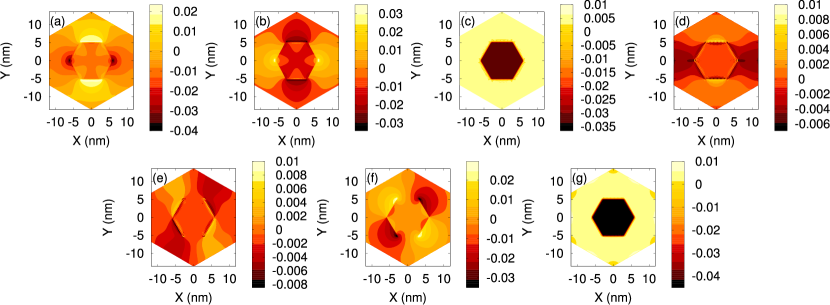
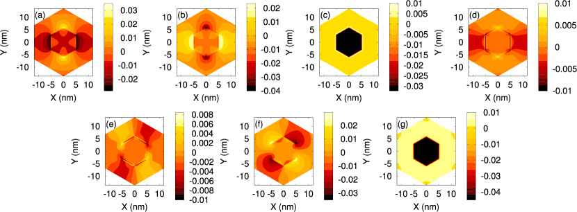

Figures 4 to 6 show the strain fields in the -plane for an infinite wire modeled using the VFF model and three different core-shell geometries. The strain of the hexagonal geometry (depicted in Figs. 1 and 2) is displayed in Fig. 4. All strains are given with respect to the nanowire oriented coordinate system (). Corresponding plots for a parallel hexagonal geometry, where the core hexagon is rotated by relative to that of Fig. 2, and for a cylindrical geometry, are shown in Figs. 5 and 6. In all cases the nanowire is composed of a GaAs core and a GaP shell. We discuss the strain components in the hexagonal geometries, and then compare with the cylindrical geometry.
IV.1.1 Axial Strain
As discussed in Sec. II.3.1, we see in several of the figures that the strain is discontinuous at the core-shell interface. The axial strain is displayed in Fig. 4(c), and we see that it is constant within core and shell (as was used in the infinite CE model). The core material (GaAs) has a larger lattice constant than the shell material (GaP), and the energetically most favorable core-shell nanowire configuration will have an interatomic spacing that is in between those of bulk GaAs and bulk GaP. We therefore see an axial compression () of the core and an axial tension () of the shell.
IV.1.2 Hydrostatic Strain
IV.1.3 Planar Tensile Strains
Tensile strains correspond to expansion or compression along the coordinate axes. In Fig. 4(a), , i.e., the compression in -direction, is shown. The structure is compressed in the direction everywhere along the -axis. The core is compressed, as it has to fit into a space too small for it to be at equilibrium, and the shell is compressed along this axis because it is pushed outwards by the core. Along the -axis, the core is again everywhere compressed, but the shell has been expanded relative to its equilibrium state. As discussed for the axial strain, the equilibrium configuration will, parallel to an interface, have an interatomic spacing in between those the two materials take in bulk. Therefore, the shell, with a smaller bulk lattice constant, is expanded. A trace of the same effect can be seen in the component of the strain, Fig. 4(b), near the two corners of the core with . In this case, there is no interface exactly parallel to the -axis. Nevertheless, the effect is still visible at the corners. In Fig. 5(b), the core has been rotated by relative to the geometry of Fig. 4(b). In this case, there is an edge of the core-shell interface parallel to the axis, and we see an expansion in the shell close to that edge.
IV.1.4 In-plane Shear Strain
The shear strains , and are nonzero if the local deformation changes the angles between the basis vectors. Considering the lower left part of Fig. 4(f), and applying the same argument we used for the strain components and , we expect radial compression and circumferential extension of the shell, and we see a nonzero planar shear strain . The negative value corresponds to the fact that the right angle between the unit vectors and is locally enlarged by the deformationNye (1985). Analogously, in the upper left part of the same figure, the angle between and is locally shrunk, and this corresponds to a positive value for .
IV.1.5 Warp Effect
The nonzero values for and , shown in Fig. 4(d) and Fig. 4(e), correspond to the fact that a cross section in the -plane is warped into a non-flat surface in the strained wire. In other words, when the core pushes outwards on the shell, it is energetically favorable for the shell to respond by not only becoming compressed radially, but also to deform by warping out of the -plane.
IV.1.6 Cylindrical Geometry
Fig. 6 shows numerical results for a cylindrical nanowire geometry. The general features are similar to the previously described geometries. The symmetry of the strain due to the zinc blende lattice can be seen more clearly in the cylindrical geometry. Figures 6(a) and (b) show that and are almost identical in the shell, except for the sign. In a significant part of the shell, they are larger in magnitude than both the axial [Fig. 6(c)] and the hydrostatic [Fig. 6(f)] strains. We note also that the warp strains, shown in Fig. 6(d) and Fig. 6(e), do not vanish in the cylindrical wire. Thus, the warp effect is not solely an artefact of the hexagonal nanowire geometry, but an effect of the zinc blende lattice structure.
IV.2 Linescans

In Fig. 7, strain components are plotted along paths which are parallel to the nanowire axis. The solid line corresponds to a path in the core [], and the dotted line corresponds to a path in the shell [].
As discussed previously, far away from the free ends, the strain converges towards its value in an infinite nanowire. We find that, for points that lie more than 30 nm away from the ends of our finite nanowire, no strain component deviates by more than from its value at the center of the finite nanowire (). We interpret this as an indication that our nanowire geometry has sufficient length and that the strain field at will correspond to the strain field in the infinite model.
The behavior of the strain as a function of can be understood as a combination of two effects. The first effect is due to the hexagonal core-shell geometry and the zinc blende lattice structure and was discussed above. The second, the Poisson effect, dominates the strain in the vicinity of the free ends. The core of the wire is radially compressed by the shell, and responds by expanding significantly along the axial direction. Far from the ends, this expansion is prevented by the shell, and the core is axially compressed, as seen in the plot of in Fig. 7. Close to the free ends, the core bulges out of the wire, giving the end-surfaces of the nanowire slightly convex shapes. This allows the core to relax more, as is seen in the same plot, where the magnitude of decreases towards the end of the wire. The Poisson effect is responsible for the main features of the -dependence of the other strain components as well.
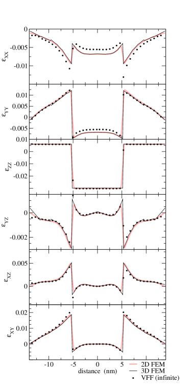
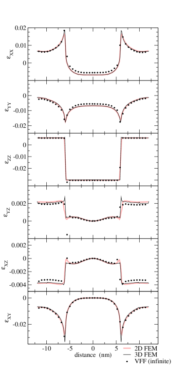
Figures 8 and 9 show a comparison between the strains of the different models along paths in an -plane. The model not shown is the VFF model for a finite wire. Far from the ends, this model agrees well with the infinite VFF model. We observe that the results from the continuum models for finite and infinite wires are very similar.
Deviations between the VFF and CE models at the core-shell interfaces are expected. These deviations are unphysical, in the sense that macroscopic strain is a locally defined phenomenon within a homogeneous material. We also see significant systematic deviations between the VFF and CE models inside the core, and we attribute these to the discrepancy in effective elastic constants of the VFF and CE models. As a test of this, we compared calculations from the CE and VFF models, where we tuned the parameters of the CE model so that the two models used the same effective elastic constants. A comparison of the strain fields from those calculations showed good agreement between the VFF and CE models (comparable to the agreement between our finite and infinite models).
V Conclusions
We have given a self-contained comprehensive account of our computations of strain distributions in finite and infinite core-shell nanowires with lattice mismatch using both continuum-elasticity theory and an atomistic VFF model. The strain profiles were shown in Figs. 4 to 9 and were discussed. The atomistic VFF model has in this work been formulated within a unit cell of a nanowire with periodic boundary conditions in the axial direction. A corresponding continuum elasticity model for an infinite wire was also defined in a unit cell. Finally, a long and finite wire was studied using the continuum-elasticity theory and the VFF model.
We observe bulging effects at the free ends of the finite wires and find good agreement between results at a cross section of a finite wire far away from its ends and at a cross-section of an infinite wire. The strain distributions obtained in the calculations using the continuum and atomistic models show qualitatively good agreement. Quantitatively, deviations remain, but their origin was discussed. In contrast to the hydrostatic strain, which has a very simple structure, the individual strain components have very complex structure. The non-planar shear strains are generally smaller than the diagonal components, but non-vanishing. The strain in the core is dominated by the axial strain, but at the core-shell interface and just outside it, a richer structure is found in the strain distributions.
Future work will consist of computing properties such as electronic structure and phonons based on the results presented here. In those calculations, extensions to multi-shell structures and heterostructures combining zinc blende and wurtzite crystals will be considered.
Acknowledgements.
N.S. and J.G. thank the Swedish Research Council for financial support. F.B acknowledges the financial support from the Academy of Finland.References
- Huang et al. (2001) Y. Huang, X. Duan, Y. Cui, L. Lauhon, K. Kim, and C. Lieber, Science 294, 1313 (2001).
- Law et al. (2005) M. Law, L. Greene, J. Johnson, R. Saykally, and P. Yang, Nature Materials 4, 455 (2005).
- Wang et al. (2008) K. Wang, J. Chen, W. Zhou, Y. Zhang, Y. Yan, J. Pern, and A. Mascarenhas, Adv. Mater. 20, 3248 (2008).
- Huang et al. (2005) Y. Huang, X. Duan, and C. Lieber, Small 1, 142 (2005).
- Zheng et al. (2005) G. Zheng, F. Patolsky, Y. Cui, W. Wang, and C. Lieber, Nature Biotechnology 23, 1294 (2005).
- Lauhon et al. (2002) L. J. Lauhon, M. S. Gudiksen, D. Wang, and C. M. Lieber, Nature 420, 57 (2002).
- Skold et al. (2005) N. Skold, L. Karlsson, M. Larsson, M.-E. Pistol, W. Seifert, J. Tragardh, and L. Samuelson, Nano Letters 5, 1943 (2005).
- Schrier et al. (2007) J. Schrier, D. O. Demchenko, Wang, and A. P. Alivisatos, Nano Letters 7, 2377 (2007).
- Zhang et al. (2007) Y. Zhang, Wang, and A. Mascarenhas, Nano Letters 7, 1264 (2007).
- Boxberg and Tulkki (2007) F. Boxberg and J. Tulkki, Rep. on Progr. in Phys. 70, 1425 (2007).
- Csontos et al. (2008) D. Csontos, U. Zülicke, P. Brusheim, and H. Q. Xu, Phys. Rev. B 78, 033307 (2008).
- Csontos et al. (2009) D. Csontos, P. Brusheim, U. Zülicke, and H. Q. Xu, Phys. Rev. B 79, 155323 (2009).
- Persson and Xu (2002) M. P. Persson and H. Q. Xu, Appl. Phys. Lett. 81, 1309 (2002).
- Persson and Xu (2004a) M. P. Persson and H. Q. Xu, Phys. Rev. B 70, 161310 (2004a).
- Persson and Xu (2004b) M. Persson and H. Xu, Nano Letters 4, 2409 (2004b).
- Persson and Xu (2006a) M. P. Persson and H. Q. Xu, Phys. Rev. B 73, 125346 (2006a).
- Persson and Xu (2006b) M. P. Persson and H. Q. Xu, Phys. Rev. B 73, 035328 (2006b).
- Eshelby (1957) J. D. Eshelby, Proc. R. Soc. London, Ser. A 241, 376 (1957).
- Stangl et al. (2004) J. Stangl, V. Holý, and G. Bauer, Rev. Mod. Phys. 76, 725 (2004).
- Niquet (2006) Y. M. Niquet, Phys. Rev. B 74, 155304 (2006).
- Niquet (2007) Y. Niquet, Nano Letters 7, 1105 (2007).
- Pistol and Pryor (2008) M.-E. Pistol and C. E. Pryor, Phys. Rev. B 78, 115319 (2008).
- Keating (1966a) P. N. Keating, Phys. Rev. 145, 637 (1966a).
- Nye (1985) J. Nye, Physical Properties of Crystals (Clarendon, Oxford Eng., 1985).
- Vurgaftman et al. (2001) I. Vurgaftman, J. R. Meyer, and L. R. Ram-Mohan, J. Appl. Phys. 89, 5815 (2001).
- Povolotskyi and Carlo (2006) M. Povolotskyi and A. D. Carlo, J. of Appl. Phys. 100, 063514 (2006).
- Cleland (2003) A. Cleland, Foundations of nanomechanics (Springer, Berlin, 2003).
- Søndergaard et al. (2009) N. Søndergaard, Y. He, C. Fan, R. Han, T. Guhr, and H. Q. Xu, J. Vac. Sci. Technol. B 27, 827 (2009).
- Zienkiewicz and Taylor (1989) O. Zienkiewicz and R. Taylor, The Finite Element Method, vol. 1 (McGraw-Hill, London, 1989).
- Pryor et al. (1998) C. Pryor, J. Kim, L. W. Wang, A. J. Williamson, and A. Zunger, J. of Appl. Phys. 83, 2548 (1998).
- Martin (1970) R. M. Martin, Phys. Rev. B 1, 4005 (1970).
- Keating (1966b) P. N. Keating, Phys. Rev. 149, 674 (1966b).
- Cousins (2003) C. S. G. Cousins, Phys. Rev. B 67, 024107 (2003).
- (34) Another 1/6 of the wire is obtained through a reflection of the simulated 1/6, and the remaining two thirds of the geometry are then obtained as rotated copies of the previously obtained third of the wire.