Homogenization-based Analysis of Quasicontinuum Method for Complex Crystals
Abstract
Among the efficient numerical methods based on atomistic models, the quasicontinuum (QC) method, introduced by Tadmor, Ortiz, and Phillips (1996), has attracted growing interest in recent years. Originally, the QC method was developed for materials with simple crystalline lattice (simple crystals) and later was extended to complex lattice (Tadmor et al, 1999). In the present paper we formulate the QC method for complex lattices in a homogenization framework and perform analysis of such a method in a 1D setting. We also present numerical examples showing that the convergence results are valid in a more general setting.
1 Introduction
In some applications of solid mechanics, such as modeling cracks, structural defects, or nanoelectromechanical systems (NEMS), the classical continuum description is not suitable, and it is required to utilize an atomistic description of materials. However, full atomistic simulations are prohibitively expensive, hence there is a need for efficient numerical method. Among the efficient methods based on atomistic models, the quasicontinuum (QC) method has attracted growing interest in recent years [24].
The QC method is a multiscale method capable of coupling atomistic and continuum description of materials. It is intended to model an atomistic material in a continuum manner in the regions where deformation variations are low and use fully atomistic model only in the small neighborhood of defects, thus effectively reducing the degrees of freedom of the system. Originally, the QC method was developed for materials with simple crystalline lattice [32] and the convergence of a few variants of the method has been analyzed under some practical assumptions (see, e.g., [14, 25, 22, 27]). The QC method is based on the so-called Cauchy-Born rule (see, e.g., [18, 20, 16, 8]) which states that the energy of a certain volume of material can be approximated through the deformation energy density, which is computed for a representative atom assuming that the neighboring atoms follow a uniform deformation. Later, QC was extended to materials with complex lattice (a union of a number of simple lattice sites) [33] based on the improved Cauchy-Born rule [31] which accounts for relative shifts between the comprising simple lattice sites. Examples of such materials include diamond cubic Si, HCP metals (stacking two simple hexagonal lattices with a shift vector) like Zr, ferroelectric materials, salts like Sodium Chloride, and intermetallics like NiAl. Recent developments of QC for complex lattices also include adaptive choice of representative cell of complex crystals [13]. It appears that no rigorous analysis is available so far for the complex lattice QC.
In the present work we propose a treatment of complex crystalline materials within the framework of discrete numerical homogenization. Homogenization techniques for partial differential equations (PDEs) with multiscale coefficients are known to be successful for obtaining effective equations with coefficients properly averaged out [7]. Finite element methods based on homogenization theory have been pioneered by Babŭska [4] and have attracted growing attention these past few years (see [21, 2, 15, 17] for textbooks or review papers). Following the ideas of [7], we use homogenization techniques to describe the coarse-graining of complex lattice. This allows to give a new formulation of the QC method for complex lattice (that we will sometimes call “homogenized QC” (HQC) method). More interestingly, we find that there is equivalence between the discretely homogenized QC and the complex lattice QC based on the improved Cauchy-Born rule. We can then use this discrete homogenization as a framework for the description of a quasicontinuum method for complex materials. There are several benefits in this regard. First, in this framework the connection to the well-developed theory of continuum homogenization and related numerical methods becomes more apparent. This allows us to apply the analysis techniques developed for continuum homogenization [2, 15] to the quasicontinuum method for complex materials. Second, homogenization theory can be used to upscale the atomistic model in both, time and space, which makes it promising for modeling and especially analyzing zero temperature and finite temperature motion of atomistic materials [15, 19, 24]. Also, homogenization can be applied to “stochastic” materials, atomistic counterparts of which include polymers [6] and glasses. Last, for the finite temperature simulations, when materials are modeled with static atoms interacting with effective temperature-dependent potentials, homogenization may serve as a rigorous instrument to derive such potentials.
We note that the idea of applying homogenization to atomistic media has appeared in the literature [11, 12, 9, 19, 6]. We also note that the method considered in this paper is essentially equivalent to the QC for complex crystals, being put in the framework of numerical homogenization.111For more details on relations of different multiscale methods for complex crystalline materials, refer to the companion paper [3]. However, the rigorous discrete homogenization procedure and related numerical method allow us to derive error estimates for the homogenized QC method, when compared to the solution of discretely homogenized atomistic equations. It also allows, by a reconstruction procedure, to approximate the original full atomistic solution. To the best of our knowledge, such error estimates are new. As in many numerical homogenization techniques for PDEs, there is no need for our numerical approximation to derive homogenized potential before-hand, since the effective potential is computed on the fly (see, e.g., [15]). Finally, we note that the error estimates are derived in one dimension for linear interaction, but the numerical methods itself applies to nonlinear multi-dimensional problems. Numerical experiments show that the derived estimates are valid in more general situations.
The paper is organized as follows. After a brief presentation of a 1D model problem of atomistic equilibrium (Section 2) we discuss discrete homogenization (Sections 3 and 4), and then formulate and analyze a macro-micro numerical method capable of capturing effective behavior of a complex material (Sections 5 and 6). We also illustrate how the presented technique can be applied to 2D crystals (Section 7). Numerical examples illustrating the performance of our method are then presented (Section 8), followed by concluding remarks (Section 9).
1.1 Function spaces
We consider the space of -periodic functions on the lattice (, ):
and the space of -periodic sequences with zero average:
where the discrete integration operator is defined for by
Likewise, we consider the tensor product space on :
and discrete integration operators
A bilinear form for is defined by
and for by
For we introduce the forward discrete derivative
and the -step discrete derivative ()
In addition to differentiation operators, we define for , the translation operator
Then the -step translation () can be expressed as a power of :
The definitions of the discrete derivative and translation generalize to functions in by considering the partial discrete derivative and translation operators, i.e., applied to and applied to .
The following lemma, whose proof is trivial, will be useful:
Lemma 1 (Discrete integration by parts).
For the following identity holds:
This identity can be written in an operator form as .
We finally define appropriate norms for functions :
| (1) |
1.1.1 Identification in
It is clear that a function can be identified with a representant in , where (the subscript per means that is defined by periodic extension for all indices ). We can also identify functions in with their representants in with zero mean. We will denote this vector space as . In this paper we will use a product space of with different values of . In such a case it is important to retain the functional notation for . However, when there is no confusion, we will avoid such heavy notations and simply use where due to identification of with , the operators are defined as
| (2) |
will simply be denoted as . Likewise the discrete integration and bilinear form can be written as
The notation denotes the component-wise product: which will enable us to conveniently write . A scalar will sometimes be identified with the vector . Finally, for the norms previously defined on , we will use the following notations for :
When it will cause no confusion, we will omit the argument in the norms, thus writing only , , etc.
2 Problem Formulation
The focus of the present study is on correct treatment of atomistic materials with spatially oscillating or inhomogeneous local properties. For simplicity, we will first consider the 1D periodic case (the 2D case will be discussed in Section 7).
2.1 Equations of Equilibrium
We describe the formulation of the problem of finding an equilibrium of an atomistic material in the 1D periodic setting. We consider the periodic boundary conditions in order to avoid difficulties arising from presence of the boundary of the atomistic material. Otherwise, the boundary of an atomistic material, unless properly treated, would contribute an additional error to the numerical solution, studying which is not an aim of the present work. Nevertheless, it should be noted that the numerical method and the algorithm proposed in the present work can be applied to Dirichlet, Neumann, or other boundary conditions.
Consider a material at the microscopic scale which occupies a domain . We assume that the position of the atoms in reference configuration is given by When the material experiences a deformation the atom positions become . We assume that the displacements behave periodically with a period length , i.e.,
| (3) |
Setting (see Section 1.1.1) we see that . According again to Remark 1.1.1 we will identify with for the discussion which follows.
We assume that the atoms interact through the pairwise potential , which depends on particular atoms and thus allowing for modeling heterogeneous materials. Due to the assumption of periodic displacements we have The energy of atomistic interaction of the system (summed for the atoms over one period) is then
We assume that the potential vanishes for large enough, so that it is sufficient to consider at most neighboring atoms in the interaction energy:
where are introduced in the following way:
| (4) |
The potential energy of the external force is
The forces on each atom are given and considered to be independent of actual atom positions . For the problem to be well-posed, the sum of all forces per period is assumed to be zero, i.e., .
The total potential energy of the atomistic system is then
In these notations the problem of finding the equilibrium configuration of atoms can be written as
| (5) |
For the equations (5) to have a unique solution, we must additionally require that the average of is zero:
| (6) |
The equilibrium equations (5) together with the additional condition (6) can be written in variational form: find such that
| (7) |
where
| (8) |
Thus, the variational form of the problem (7) is
| (9) |
As written in this form, the variational equation (9) resembles the nonlinear continuum equation
The problem (9) is often solved with the Newton’s method. It consists in choosing the initial guess and performing iterations to find . For that, the equations (9) are first linearized on the solution :
| (10) |
and then solved for the next approximation until two successive iterations give close results. Here, according to (4) and (8), is given by
Notice that we have identified here the diagonal Jacobian matrix with a vector in and used the component-wise product between two vectors (see Section 1.1).
2.2 Linearized Model and Nearest Neighbor Interaction
We can linearize the problem in a neighborhood of a given displacement :
Hence upon defining
| (11) |
we can use the linearized approximation
Here we used the formula of integration by parts (Lemma 1) and again the component-wise product for . We see that in the case of linear interaction, the term with can be absorbed into the external force , which turns the generic equilibrium equations (7) to
| (12) |
If we further assume that only nearest neighboring atoms interact (i.e., that ), then the equations (12) are further simplified to
| (13) |
where we denote (i.e., for ). It will sometimes be convenient to use a “strong form” of (9) or (17), i.e., find such that
| (14) |
which is derived using Lemma 1.
3 Homogenization of Atomistic Media
We come now to the main subject of this paper, the treatment of materials with heterogeneous atomistic interaction as illustrated in Figures 1 and 2.


Naive coarse graining for such models (e.g., as given by the straightforward application of the quasicontinuum method) fail to give the correct answer. One way to treat such problems is to apply the so-called Cauchy-Born rule for complex lattices [31, 33, 30, 13]. We present here another coarse graining strategy based on homogenization ideas. We derive below a discrete homogenization of the atomistic material which will be the basis for formulating and analyzing a quasicontinuum method for complex lattices. We note that our approach is different from the approach chosen in other works discussing homogenization of atomistic media [9, 10, 19], which consists in treating the homogenized material at the continuum level and the heterogeneities at the atomistic level (the idea of continuous and discrete can also be seen in the proof of the main results in [16]). In our approach, the homogenized material will retain its atomistic description. In this section we derive the homogenized equation using asymptotic expansion. Rigorous justification of the homogenized limit will be given in Section 4 by means of error estimates towards the full atomistic solution.
3.1 Asymptotic expansion
We will assume that the local heterogeneity of the atomistic interaction is periodic with period . In order to take into account the local variation of the atomistic interaction we think of the displacement as depending on a fast and a slow scale . We define , the macro (“slow”) variable, and , the micro (“fast”) variable, and consider functions indexed by As we consider periodic local interaction (with period ) we assume that the functions are -periodic in the fast variable, i.e., they satisfy
while the behavior w.r.t. is similar to the previously considered
Recalling the definitions of Section 1.1, this means . We then consider the asymptotic expansion
| (15) |
In addition to the discrete derivative, translation, and integration, defined in Section 1.1 we need the total derivative and the total -step derivative of a function :
A simple calculation shows that the total derivative and the total -step derivative can be expressed in terms of , the discrete partial derivatives and translation operator defined in Section 1.1, in the following way:
| (16) | |||||
3.2 Homogenization for Nearest Neighbor Linear Interaction
In this subsection we will perform the asymptotic analysis for the equation of equilibrium of atomistic materials. To explain our procedure, we first treat the simplest interaction model, i.e., the case of nearest neighbor linear interaction. Asymptotic expansion and homogenization procedure for more general cases will be given in the following subsection. We consider the problem (13), written in functional form ():
| (17) |
with defined as follows:
where the function , i.e., the tensor is “-periodic” in the variable. We assume that the function is uniformly positive in the following sense:
| (18) |
We also assume that the external force it does not depend on , i.e., . We emphasize that oscillatory external forces could also be considered. The homogenized equation would then depend on a proper average of the external forces. For simplicity we will not consider this case. We now proceed as in the “classical homogenization” [5, 7, 28] and plug the ansatz (15) in (14) (we will go back and forth from the variational formulation (17) to the strong formulation (14)). This gives
| (19) | |||||
Here we used the identity (16), and Lemma 1 to compute the adjoint . We thus obtain a cascade of equations and collect powers of .
Collect the terms in (19):
Thanks to (18) we have . This implies that is independent of and only a function of , i.e.,
We next collect the terms in (19):
| (20) |
where we have used the fact that does not depend on , which implies and . As usual in homogenization we take advantage of the separation of variables of the right hand side of (20) and we let be the solution of
| (21) |
In view of (18), this problem has a unique solution (up to an additive constant) if and only if (solvability condition) which indeed holds due to the periodicity assumption on . Existence and uniqueness follows from the Lax-Milgram theorem for the following variational problem (see Lemma 2): find such that
| (22) |
It is then readily seen that solves (20). The general solution of this latter equation involves a constant depending on determined by the condition (recall that functions in the space have zero average), i.e.,
Finally, collecting the terms in (19) gives
The solvability condition for the existence of a solution reads
leading to the homogenized equation
| (23) |
where we choose, as for the original problem (17), the periodic boundary conditions and where
| (24) |
Thus, we obtained the equation for the homogenized displacement with the homogenized discrete tensor . The homogenized tensor no longer depends on the fast variable and therefore we can apply the standard QC method to the homogenized equation (23). The equation (23) has to be supplemented with boundary conditions. Our choice of periodic boundary conditions for the displacement (see (3)) leads to searching for .
In the simple case of nearest neighbor linear interaction, the homogenized discrete tensor can be found analytically. Indeed, from (21) we see that does not depend on :
| (25) |
from where we find
| (26) |
The constant of integration can be found by averaging (26) over :
from where we find
| (27) |
and the homogenized tensor is thus
| (28) |
Thus the homogenized equations (23) are written as
We emphasize that this procedure and the obtained results are well-known for PDEs [7, Chap. 1].
3.3 Generalizations
Below we generalize the results of the previous subsection to the cases of finite range (i.e., ) linear (Section 3.3.1) and nonlinear (Section 3.3.2) interaction, omitting this details of technical nature.
3.3.1 Finite Range Linear Interaction
One technical difficulty in this case is that there are different differentiation operators . Then a straightforward generalization of the results of the previous subsection would yield depending on discrete “macroscale” derivatives (). This approach would also essentially differ from the results in continuum homogenization. Therefore, instead of the identity
| (29) |
the following approximate (accurate to ) identity should be used:
| (30) |
The accuracy of is enough if one seeks to obtain only the homogenized solution and the leading term of the correction .
The procedure can now be performed similarly to the nearest neighbor interaction case: we plug the ansatz (15) in (12). As previously, we obtain that and the terms yields
where is a solution of
| (31) |
Appropriate conditions on are required to ensure that (31) has a unique solution. Collecting the terms using the solvability conditions for (similarly to the nearest neighbor case) yields the homogenized equation
where the homogenized tensor is defined as
A remarkable feature of the result of homogenization of material with finite range interaction is that the material thus homogenized contains only the nearest neighbor interaction despite the original model having longer interactions. This is a consequence of our choice of in the form (30). If we would have chosen the exact relation (29), then the homogenized material would contain the same number of interacting atoms.
3.3.2 Finite Range Nonlinear Interaction
In this subsection we further generalize the results to the case of a general nonlinear material (9)
We assume that the nonlinear tensor has the form and set as previously. In accordance with the definition (8) it means that the interacting potential depends on and and
We again proceed with the asymptotic expansion. We use the ansatz (15) (we directly assume that in order to simplify the argument), the approximation (30) in the above nonlinear equation and identify the power of . This yields the homogenized equation
where
The function solves the parametric problem
| (32) |
Of course, structure assumptions on are needed to ensure a unique solution of (32). We will not go into details here as our analysis in Section 4 and 5 will be limited to the linear case.
Remark 1.
It is useful to highlight one more feature of the homogenized equations, before we proceed with describing the numerical algorithm. In terms of atomistic interaction potential the homogenized tensor is
This representation can be interpreted as the averaging of the functional derivative of the original energy
at the corrected solution . This fact is important in showing the equivalence between QC applied to homogenized material and QC for complex lattices [33] and will be proved in the companion paper [3].
4 Analysis of Equations
In this section we show that the original and the homogenized problems of equilibrium of materials with spatially oscillating properties are well-posed and that the difference between their solutions is in the appropriate norms. We limit our analysis to the case of nearest neighbor linear interaction in the 1D periodic setting, but allow the material properties to vary. Such interaction corresponds to the nonlinear interaction linearized on a given non-uniform deformation.
After defining the appropriate norms for measuring the error (Section 4.1), we state the main theorems (Section 4.2) followed by proof of technical lemmas (Section 4.3).
In this section, by , , , we denote generic constants which may depend on , , , and , but are independent of .
4.1 Preliminaries
Let be the solution of (17). We assume as in the previous section that the tensor can be written as
| (33) |
where the function (i.e., is “-periodic” in the variable). This holds, for instance, if we linearize the interaction the original nonlinear model on the displacement (cf. (11)) that can be expressed as . We also assume that satisfies
| (34) | |||
| (35) |
Let be the solution of (23) where the homogenized tensor is given by
and is a solution of (21). It clearly follows from (34) that is also coercive and bounded, i.e.,
| (36) |
The existence and uniqueness of a solution of (17) (24), and (21) follow from standard arguments. For the sake of completeness we briefly sketch the proof.
Proposition 1.
Proof.
Proof.
The problem (21) can be written as follows: find such that
| (39) |
As is -periodic in the variable, we have and the existence and uniqueness of a solution (depending on ) can be established as in Proposition 1. Notice that depends on . As the equation (39) remains unchanged when is changed to , we also have . ∎
4.2 Main results
We start with formulating the following two technical lemmas that will be proved in Section 4.3.
Lemma 2.
In what follows, a function of two variables (e.g., ) may be identified with a corresponding function of one variable (). Whenever it may cause confusion we will explicitly specify the function space or the norm (i.e., or ).
Lemma 3.
Theorem 1.
Proof.
To show (46) we need to estimate the right-hand side of (45):
where we used (43), (38), and (43) to estimate , and , respectively, and also (87) (Lemma 14) to estimate through . Notice that we used the estimate
which can be obtained with the help of (36):
by estimating the terms , , and using (23), (42), and (37), respectively.
Theorem 2.
Assuming the hypotheses of Theorem 1, there exists a constant such that
Proof.
4.3 Proof of Technical Lemmas
Proof of lemma 2..
5 Homogenized QC for Complex Lattices
We formulate the homogenized quasicontinuum method (HQC) — the QC method for complex crystalline materials — in a framework of homogenization. We introduce HQC in the general 1D periodic case, i.e., with finite range nonlinear interaction (see (9)), and possibly oscillating external force . For the case of materials with known periodic structure (i.e., crystalline materials), the HQC method will be equivalent to applying QC to the homogenized equations. We mention however two advantages of HQC. First, the method is based on the original equation describing the spatially oscillating material and does not rely on effective (homogenized) equation derived beforehand. Such strategies have proved successful in the continuum elasticity where many macro to micro methods averaging the effective equations on the fly have been derived (see the review paper [21] and the references therein). Second, we think that the HQC can be applied to non-crystalline materials and to time-dependent zero- or even finite-temperature problems.
5.1 HQC Method
Consider the problem of finding an equilibrium of an atomistic material in the general 1D periodic case (i.e., with finite range nonlinear interaction) (9). The method will be presented using macro-to-micro framework as used in some numerical homogenization procedures [2, 15, 23, 21, 34].
5.1.1 Macroscopic affine deformation
Let
be the reference lattice for the problem (9). In the set of indices we choose values () and compose a macroscopic lattice
defining the macroscopic partition of the interval
Here we fix for convenience (we can do so without loss of generality due to translation invariance) and define in accordance with the periodic extension, define (for ) the length of the , and . We define the space of piecewise affine (discrete) deformations by
and
5.1.2 Sampling Domains
Inside each macroscopic interval we choose a representative position and a sampling domain
and define the operator of averaging over the sampling domain
The sampling domain should be chosen closer to the center of the interval if the material’s properties vary within the interval (more precisely, if the interaction potentials for different groups of adjacent atoms are different), as we will see in Theorem 6. More sampling domains per macro interval may be considered for higher-order macro element space .
5.1.3 Energy and Macro Nonlinear Form
Define the energy of the HQC method
where , defined by (49), is the microfunction constrained by in the sampling domain , and is the energy of interaction of atoms and (i.e., in the notations of Section 2, cf. (4)).
The functional derivative of the above energy reads
| (48) |
where is the derivative of the reconstruction , and is defined in accordance with (8).
5.1.4 Microproblem
Given a function is a function defined on such that and
| (49) |
Remark 2.
Remark 3.
In the case of linear interaction, the reconstruction is a linear function and hence , which makes the derivative of the HQC energy (48) take the form
| (50) |
5.1.5 Reconstruction
The function is defined on . We define an extension of on by periodic extension outside :
| (52) |
where , and is an integer value modulo . By extending the function in each , one obtains a function defined on which we denote by .
5.1.6 Variational Problem
5.2 HQC Algorithm
The problem (53) is nonlinear and its practical implementation is usually done by the Newton’s method. We briefly sketch below an algorithm for solving (53).
5.2.1 Second Derivative of the Energy
5.2.2 Newton’s Iterations for the Macroproblem
The algorithm based on the Newton’s method consist in choosing the initial guess and performing iterations
| (56) |
until becomes close to in a chosen norm.
To solve the linear system (56) for , we choose a nodal basis () of . One way to satisfy the condition would be to perform all the computations with one basis function eliminated (e.g., to consider for ), and post-process the final solution as .
5.2.3 Solution of the Microproblem
The microproblem (49) can also be solved with Newton’s method. For that, one needs to choose an initial guess to , for instance and solve
with respect to constrained by , until the difference between and is small in a chosen norm.
After that, we can compute by solving
| (57) |
constrained by . Notice that the derivative of the basis functions on the interval can either be (in which case equals zero identically), or . It implies that we essentially need to solve the problem (57) limited number of times (once in the 1D case, or between and in , depending on implementation).
Also observe that when computing , we need to invert the same linear operator as in the final Newton’s iteration, which allows for some additional optimization.
5.3 Possible Modifications of the Algorithm
First, notice that when solving for we could linearize the problem on the previous iteration . In that case we would have only the linear cell problems and thus we would need only outer Newton’s iteration, but it would be required to keep the values of the micro-solution from the previous iteration. Moreover, even in a practical implementation of the above algorithm it may be required to keep the values of the micro-solution: one needs these values to initialize the inner Newton iterations [33].
Another modification could be to compute the contribution of the external force in (54) for a single atom in the case of no oscillations in .
In the case of linear interaction, the algorithm becomes simpler: one does not need to do Newton iterations. Nevertheless, even if the algorithm in subsection 5.2 is applied to the linear problem, the Newton’s method would converge in just one iteration.
6 Convergence of HQC
In this section we study convergence of the HQC method introduced in (53). We analyze the method for linear problems and nearest neighbor interaction (17). We treat the external force in an exact manner. We furthermore make a slight modification to the HQC method: we assume (33) and collocate the tensor in (50) and (49) in the slow variable at in each sampling domain . That is, we solve
| (58) |
where
| (59) |
| (60) |
For an illustration of a collocation point and a sampling domain refer to Figure 3.

In order to obtain the second order convergence in the -norm, we will assume two additional conditions:
| (61) |
| (62) |
The condition (61) states that the collocation point is at most away from the center of each .
In this section, the constants , , etc., denote generic constants which may depend on , , , , , and , but are independent of and .
6.1 Main Results
Before proceeding with analysis (Section 6.2), we summarize the main convergence results. The results are formulated in terms of , the so-called modeling error, which is defined in (71).
Theorem 3.
Theorem 4.
Theorem 5.
The modeling error , defined in (71), reflects the fact that we introduce some error when neglecting the values of the tensor everywhere outside the sampling domains . The modeling error is estimated in the following theorem.
6.2 Error analysis
We start our analysis with the following lemma which asserts that the results stated in Section 6.1 can be reformulated in terms of the standard QC method applied to the homogenized equations (23). Recall the definition of the homogenized tensor
and define the collocated homogenized tensor for .
Proof.
Fix the element and notice that the reconstruction defined by (60) can be written as , where satisfies
Notice that and are constant inside each sampling domain . Upon substitution this equation takes the form
and its solution can be written as , cf. (22). Finally, noticing that periodically extending in
| (69) |
yields exactly concludes the proof of (68). ∎
Lemma 5.
Proof.
We continue the argument of the previous lemma: we first fix the element and differentiate (69) to get
Hence we compute
Finally, the following computation then shows that the left-hand side of (58) is equal to that of (70):
where we used Remark 4 in the first step of this derivation, and omitted the argument or of the functions , , and since they are constant on each interval . Thus, (58) and (70) are equivalent. ∎
Define the modeling error as
| (71) |
where is the solution of the following problem:
| (72) |
Proposition 3.
Proof.
The statement can be proved similarly to Proposition 1, by noticing that and , and substituting the original space with the discretized space . ∎
We can now prove Theorem 6.
Proof of Theorem 6..
Part (c) of the theorem is trivial: if in (59), then is constant, hence coincides with , and therefore .
The bound in part (a) is based on the following estimate:
| (74) |
where the last estimate follows from (73). The difference in (74) can be estimated as follows: for
hence . Taking now supremum over concludes the proof of part (a).
To show (b), first observe that in (70), and are constant on any interval . Therefore can be changed to any other tensor with the same average over . Hence define . Since , the solution of (70) coincides with the solution of
Hence we can use the arguments of (74) to estimate:
| (75) |
where
It is straightforward to show that averages up to
and can be effectively estimated using (61). The second terms can be estimated as
Thus, combining these estimates, one gets
Taking maximum over all ,
and substituting into (75) yields the desired result. ∎
In view of Lemma 5, we will turn to analysis of the problem (72). We next introduce the (homogenized) energy norm in the space :
Obviously, under the assumption (34), due to the estimate (36), the energy norm is equivalent to the -norm:
| (76) |
Lemma 6.
Proof.
The result follows from
which states that is the orthogonal projection (in the energy norm) of onto . ∎
Following the standard procedure for the analysis of finite element methods (FEM) we will estimate , where is the nodal interpolant of . This interpolant is defined for every function in the following way. For a partition of define a function such that
| (78) |
Then set
Thus, for we have .
Lemma 7.
The following estimate holds:
where and .
Proof.
Proof of Theorem 3.
The estimate (63) (convergence in the -norm) follows from (76), (77), Lemma 7, and (67). To prove (64) (convergence in the -norm) we use the standard duality arguments. Consider
Then
hence
∎
Lemma 8.
Proof.
Lemma 9.
Proof.
7 Example of Application to a 2D Lattice
In this section, we consider a simple 2D model to illustrate how the proposed approach can be applied to 2D materials.
7.1 Notations
All the coordinates and atom indices will be vectors with two components, for instance , . The unit vectors in our 2D space will be denoted as and . The length of a 2D vector is denoted as , the scalar product of two vectors and is denoted as .
We define the inequalities for 2D vectors in the following way: if, by definition, and (likewise for relations , , and ). Thus, means and . We will also use the associated notations for the sums, for instance .
7.2 Equations of Equilibrium
Consider a square lattice with the reference configuration of atoms given by
The position of the atoms and displacements are related through . We consider the system with -periodic () conditions . The space of such -periodic vector-valued sequences is denoted as .
Consider the following operators on :
the averaging in :
and the scalar product
Consider the linear interaction of atoms defined by a set of neighbors so that the functional derivative of the interaction energy is
where defines interaction between atoms and . Such linear interaction corresponds to a spring model with zero equilibrium length (cf. [20] for the discussion on the nonlinear model with ideal springs but with nonzero spring equilibrium length). The derivative of the external potential energy is
Thus, the equilibrium equation has the form
| (82) |
7.3 Homogenization
Homogenization of equations (82) follows Section 3. By analogy with the 1D case, we will use the term “vector-valued function” (or, in short, “function”) for rather than the term “vector field”.
7.3.1 Fast and Slow Variables
We first define the fast variable , the differentiation operators
where , , , the translation operators in :
and averaging and scalar products:
The space of -periodic functions () is denoted as and hence the functions of and belong to .
7.3.2 Solution Representation
Assume, as before, and . Then for such functions and . Same as in 1D case, use the following identity:
Then the equation (82) takes the form
| (83) |
We substitute into (83) and collect the respective powers of . As before, by collecting the and the terms we obtain that and , where the matrix-valued functions and are defined as solutions to
Collecting the terms yields
where the homogenized tensors are defined as
with denoting a identity matrix. The homogenized tensors are related to the fourth-order stiffness tensor in linear elasticity theory [1, 26, 29].
7.3.3 Example of Application of Homogenization
To illustrate how the 2D discrete homogenization works, we apply it to the following model problem. The set of neighbors is defined by (we omit the neighbors that can be obtained by reflection around ) and the interaction tensor as
Such material is illustrated in Fig. 2.
This example was motivated by the study of Friesecke and Theil [20], where a similar model was considered. Friesecke and Theil considered the model with springs similar to the one illustrated in Fig. 2, which however was nonlinear due to nonzero equilibrium distances of the springs (so that the energy of the spring between masses and is proportional to , where is the equilibrium distance). They found that with certain values of parameters the lattice looses stability to non-Cauchy-Born disturbances and the lattice period doubles (thus the lattice ceases to be a Bravais lattice).
The results, given with no details of actual derivation, are the following: The period of spatial oscillations in this case is . The function has the form (here is the identity matrix). The homogenized tensors have the form
7.4 HQC
In this subsection we sketch a formulation the HQC method based on the discrete triangular elements. Namely, we choose a partition with triangles of the original atomistic domain . The space of piecewise affine deformations is denoted as .
Inside each triangle choose a sampling rectangle of the size atoms. Define the HQC energy variation:
where is the area of the triangle, and the microfunction is defined on so that and
As before, the function can be extended on the whole triangle if required.
The variational problem to be solved thus becomes
where
8 Numerical Examples
We solve numerically several model problems to illustrate the performance of HQC. We consider the linear and the nonlinear 1D model problems (Sections 8.1 and 8.2), followed by the two 2D linear model problems (Sections 8.4 and 8.4). We also study dependence of the numerical error on , the spatial period of heterogeneity of the material (Section 8.3).
The aim of the numerical experiments is twofold. First, we verify numerically the sharpness of the obtained error for the 1D linear case. Second, we investigate whether the HQC convergence results obtained for the nearest neighbor linear interaction in 1D are valid for more general cases. The numerical results show that all theoretical conclusions made in Section 6 are also valid for finite range nonlinear interaction or for 2D problems.
8.1 1D Linear
In the first numerical example we solve the problem (9) for the linear interaction case with the period of spatial oscillation and number of interacting neighbors . The potential is defined as
where
| (84) |
Such potential is periodic, hence, as suggested by Theorem 6, . The number of atoms was , and the external force was taken as
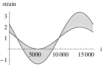
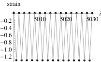
The strain for such problem is shown in Fig. 4.
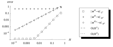
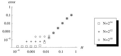
Figure 5 is aimed to illustrate theorems 4 and 5. It can be seen that the homogenized HQC solution converges to the exact solution in the -norm, does not converge in the -norm, but the post-processed HQC solution does converge in the -norm. The convergence of the homogenized solution in the -norm is exactly as suggested by Theorem 4: first it decreases with the second order as is refined, and later it stays constant as is refined further. The behavior of the lower bound of is illustrated in Fig. 6.
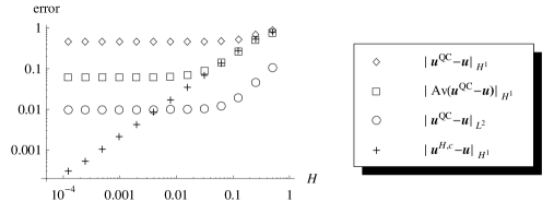
The errors of the post-processed HQC solution and the solution by the naive QC method are shown in fig. 7. It can be seen that only the solution by HQC converges to the exact solution , but the solution with the naive QC method does not converge, even when compared to the averaged exact solution (averaging operator is ) or computed in an -norm. These findings are similar to calculations of Tadmor et al [33] which show that assuming a linear interpolation for a silicon crystal greatly overestimates its strain energy density.
8.2 1D Nonlinear
We solve the problem (9) for a general nonlinear interaction case, with the period of spatial oscillation , number of interacting neighbors , and number of atoms . We chose Lennard-Jones potential
with the varying equilibrium distance
The external force was taken as
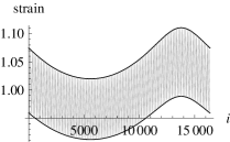
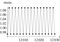
The strain for such problem is shown in Fig. 8.
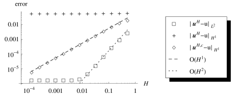
Figure 9 plots the errors of HQC in - and -norms. The results observed are qualitatively the same as the results on Fig. 7 obtained for the linear case. Also, the results of a naive application QC method to the nonlinear problem will be the same as shown on Fig. 7 for the linear case. Thus, we conclude that the convergence estimates derived for the linear case are also valid for the nonlinear case, as the conducted numerical experiments show.
8.3 Convergence for Different Periods
| 1st test case (linear) | ||||
|---|---|---|---|---|
| 2nd test case (nonlinear) |
In our analysis of the equations and the computational method, we kept the dependence on implicit, because derivation of estimates which are sharp w.r.t. is much more technical. In this section we numerically address this issue.
The first test case is similar to the one in Section 8.1. We fixed the bounds for in (84) between and and randomly generated the values of with the periods . We estimate the constant in Theorem 5 as
where the maximum is taken for . The second test case is similar to the one in Section 8.2 with randomly generated between and .
The results for both test cases are shown in Table 1. It can be seen that the constant essentially does not depend on .
This finding is important in applications, for instance, to shape memory alloys that may change their crystalline structure in the course of loading/unloading. Motivated by such applications, the authors of [13] designed the adaptive strategy of choosing , called Cascading Cauchy-Born kinematics, for the complex lattice QC method. They also presented an example of application of their method to the 1D model problem exhibiting period-doubling bifurcations. The present findings indicate that increase of period does not affect the accuracy of the method.
Independence of error bounds on is also important for modeling amorphous materials, such as glasses or polymers. Amorphous materials do not have a spatial period, instead they exhibit some random structure. By analogy with application of numerical homogenization to PDEs with random tensors, one could take large enough to capture the variation of the microscopic structure of the amorphous material, and expect that it will not affect the accuracy of representation of the macroscopic deformation as the mesh size is refined.
8.4 2D Test Case 1


We consider the example of material discussed in Subsection 7.3.3, with , , , , ,
where is determined so that the average of is zero. The total number of degrees of freedom of such system is approximately . The solution for such test case is shown in fig. 10 (the illustration is for ).

The atomistic domain is triangulated using nodes and triangles (). In each triangle a sampling domain is chosen, each sampling domain contains four atoms (see illustration in fig. 11). The number of degrees of freedom of the discretized problem is .
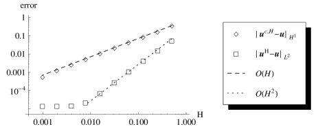
The error of the solution for different mesh size () is shown in fig. 12. The results are essentially the same as in 1D case: the method convergences with the first order of mesh size in the -norm and with the second order in the -norm. We also see the plateau for the -error of the homogenized solution . It is remarkable that all the conclusions of 1D analysis (cf. Theorems 4 and 5) are also valid for the 2D computations.
8.5 2D Test Case 2


The second test case is analogous to the previous one, but with the different tensors describing the atomistic bonds. The tensors were chosen to have the following (randomly generated) values:
For a tensor with such a random structure, the homogenized tensor can only be precomputed numerically, and in the case of a nonlinear problem should be found in the course of the actual computation. The solution (for ) is shown in fig. 13.

9 Summary and Conclusion
We have considered the problem of modeling materials with complex atomistic lattice. We have proposed a discrete homogenization framework to analyze the QC method for complex crystalline materials. This framework allowed us to prove convergence (in 1D) for the QC method proposed in [33]. Numerical homogenization has also been used to formulate the QC method. The equivalence of this algorithm to the QC method of [33] is discussed in detail in [3]. We have also shown how to apply the presented technique in a 2D setting. The 1D and 2D numerical examples presented verify validity of the analysis in more general setting. We note that the extension of the algorithm proposed in this paper to simulate atomistic materials at finite temperature or non-crystalline materials is of high interest. This is a topic for future research.
References
- [1] A. Abdulle, Analysis of a heterogeneous multiscale FEM for problems in elasticity, Math. Models Methods Appl. Sci., 16 (2006), pp. 615–635.
- [2] A. Abdulle, The finite element heterogeneous multiscale method: a computational strategy for multiscale PDEs, GAKUTO Internat. Ser. Math. Sci. Appl., 31 (2009), pp. 135–184.
- [3] A. Abdulle, P. Lin, and A. Shapeev, A review of multiscale computational methods for complex crystals, Manuscript, (2010).
- [4] I. Babuska, Homogenization and its application. Mathematical and computational problems, Numerical solution of partial differential equations, (1976), pp. 89–115.
- [5] N. S. Bakhvalov, Averaged characteristics of bodies with a periodic structure, Dokl. Akad. Nauk SSSR, 218 (1974), pp. 1046–1048. English translation: Phys. Dokl. 19, 1974–1975.
- [6] P. T. Bauman, J. T. Oden, and S. Prudhomme, Adaptive multiscale modeling of polymeric materials with Arlequin coupling and Goals algorithms, Comput. Methods Appl. Mech. Engrg., 198 (2009), pp. 799–818.
- [7] A. Bensoussan, J.-L. Lions, and G. Papanicolaou, Asymptotic Analysis for Periodic Sturcture, North Holland, Amersterdam, 1978.
- [8] X. Blanc, C. Le Bris, and P. L. Lions, Atomistic to continuum limits for computational materials science, Esaim-mathematical Modelling and Numerical Analysis-modelisation Mathematique Et Analyse Numerique, 41 (2007), pp. 391–426.
- [9] W. Chen and J. Fish, A generalized space-time mathematical homogenization theory for bridging atomistic and continuum scales, Internat. J. Numer. Methods Engrg., 67 (2006), pp. 253–271.
- [10] , A mathematical homogenization perspective of virial stress, Internat. J. Numer. Methods Engrg., 67 (2006), pp. 189–207.
- [11] P. Chung, Computational method for atomistic homogenization of nanopatterned point defect structures, Int. J. Numer. Meth. Engng., 60 (2004), pp. 833–859.
- [12] P. Chung and R. Namburu, On a formulation for a multiscale atomistic-continuum homogenization method, Internat. J. Solids Structures, 40 (2003), pp. 2563–2588.
- [13] M. Dobson, R. S. Elliott, M. Luskin, and E. B. Tadmor, A multilattice quasicontinuum for phase transforming materials: Cascading Cauchy Born kinematics, Journal of Computer-Aided Materials Design, 14 (2007), pp. 219–237.
- [14] M. Dobson and M. Luskin, Analysis of a force based quasicontinuum approximation, Math. Model Numer. Anal., 42 (2008), pp. 113–139.
- [15] W. E, B. Engquist, X. Li, W. Ren, and E. Vanden-Eijnden, Heterogeneous multiscale methods: a review, Commun. Comput. Phys., 2 (2007), pp. 367–450.
- [16] W. E and P. Ming, Cauchy-Born rule and the stability of crystalline solids: Static problems, Arch. Ration. Mech. Anal., 183 (2007), pp. 241–297.
- [17] Y. Efendiev and T. Y. Hou, Multiscale finite element methods, vol. 4 of Surveys and Tutorials in the Applied Mathematical Sciences, Springer, New York, 2009. Theory and applications.
- [18] J. L. Ericksen, On the Cauchy-Born rule, Math. Mech. Solids, 13 (2008), pp. 199–220.
- [19] J. Fish, W. Chen, and R. Li, Generalized mathematical homogenization of atomistic media at finite temperatures in three dimensions, Comput. Methods Appl. Mech. Engrg., 196 (2007), pp. 908–922.
- [20] G. Friesecke and F. Theil, Validity and failure of the Cauchy-Born hypothesis in a two-dimensional mass-spring lattice, J. Nonlinear Sci., 12 (2002), pp. 445–478.
- [21] M. Geers, V. Kouznetsova, and W. Brekelmans, Multi-scale computational homogenization: Trends and challenges, J. Comput. Appl. Math., (2010). In press.
- [22] P. Lin, Convergence analysis of a quasi-continuum approximation for a two-dimensional material without defects, SIAM J. Numer. Anal., 45 (2007), pp. 313–332.
- [23] C. Miehe and C. G. Bayreuther, On multiscale FE analyses of heterogeneous structures: From homogenization to multigrid solvers, Internat. J. Numer. Methods Engrg., 71 (2007), pp. 1135–1180.
- [24] R. E. Miller and E. B. Tadmor, The quasicontinuum method: Overview, applications and current directions, Journal of Computer-Aided Materials Design, 9 (2002), pp. 203–239.
- [25] P. B. Ming and J. Z. Yang, Analysis of a one-dimensional nonlocal quasi-continuum method, Multiscale Model. Simul., 7 (2009), pp. 1838–1875.
- [26] O. A. Oleinik, A. S. Shamaev, and G. A. Yosifian, Mathematical problems in elasticity and homogenization, Elsevier, 1992.
- [27] C. Ortner and E. Süli, Analysis of a quasicontinuum method in one dimension, M2AN Math. Model. Numer. Anal., 42 (2008), pp. 57–91.
- [28] E. Sánchez-Palencia, Non-homogeneous media and vibration theory, Springer-Verlag, 1980.
- [29] D. E. Sands, Vectors and Tensors in Crystallography, Courier Dover Publications, 2002.
- [30] G. S. Smith, E. B. Tadmor, N. Bernstein, and E. Kaxiras, Multiscale simulations of silicon nanoindentation, Acta Materialia, 49 (2001), pp. 4089–4101.
- [31] I. Stakgold, The Cauchy relations in a molecular theory of elasticity, Quarterly of Applied Mechanics, 8 (1950), pp. 169–186.
- [32] E. Tadmor, R. Phillips, and M. Ortiz, Quasicontinuum analysis of defects in solids, Philos. Mag. A, 73 (1996), pp. 1529–1563.
- [33] E. Tadmor, G. Smith, N. Bernstein, and E. Kaxiras, Mixed finite element and atomistic formulation for complex crystals, Phys. Rev. B, 59 (1999), pp. 235–245.
- [34] K. Terada and N. Kikuchi, A class of general algorithms for multi-scale analyses of heterogeneous media, Comput. Methods Appl. Mech. Engrg., 190 (2001), pp. 5427–5464.
Appendix A
Lemma 10 (Discrete Poincaré inequality 1).
Let and . Then
| (85) |
Proof.
We start with noticing that lemma A.1 in [27, p. 87] applies to and states that
where
Then with the help of the Cauchy-Schwarz inequality one obtains
where by direct computation
∎
Lemma 11.
Let . Then
Proof.
Direct computation of the right-hand-side (RHS) yields:
Notice that due to periodicity and due to average of being zero, . Hence
∎
If we consider the periodic extension of the sequence then the estimate of lemma 10 will have a slightly better constant:
Lemma 12 (Discrete Poincaré inequality 2).
Let . Then
Proof.
Corollary 1 (Discrete Poincaré inequality for ).
The functional (cf. (1)) defines a norm on . For the following inequality holds:
Lemma 13 (Inverse discrete Poincaré inequality).
For the following inequality holds:
| (86) |
for .
Proof.
∎
Lemma 14.
For the following inequality holds:
| (87) |
Proof.
Using the discrete Poincaré inequality yields:
∎