Primordial Non-Gaussianity in the Cosmic Microwave Background
Abstract
In the last few decades, advances in observational cosmology have given us a standard model of cosmology. We know the content of the universe to within a few percent. With more ambitious experiments on the way, we hope to move beyond the knowledge of what the universe is made of, to why the universe is the way it is. In this review paper we focus on primordial non-Gaussianity as a probe of the physics of the dynamics of the universe at the very earliest moments. We discuss 1) theoretical predictions from inflationary models and their observational consequences in the cosmic microwave background (CMB) anisotropies; 2) CMB–based estimators for constraining primordial non-Gaussianity with an emphasis on bispectrum templates; 3) current constraints on non-Gaussianity and what we can hope to achieve in the near future; and 4) non-primordial sources of non-Gaussianities in the CMB such as bispectrum due to second order effects, three way cross-correlation between primary-lensing-secondary CMB, and possible instrumental effects.
I Motivation
In the last few decades the advances in observational cosmology have led the field to its “golden age.” Cosmologists are beginning to nail down the basic cosmological parameters. We now know that we live in a Universe which is Gyr old and is spatially flat to about , and is made of baryons, dark matter, and remaining in the form of dark energy. Although we know the constituents to high accuracy, we still do not completely understand the physics of the beginning, the nature of dark energy and dark matter. Many upcoming CMB experiments complimented with observational campaign to map 3D structure of the Universe and new particle physics constraints from the Large Hadron Collider will enable us to move beyond the knowledge of what the universe is made of, to why the universe is the way it is. In this paper we focus on learning about the physics responsible for the initial conditions for the universe.
Inflation Guth (1981); Sato (1981); Linde (1982); Albrecht and Steinhardt (1982) is perhaps one of the most promising paradigms for the early universe, which apart from solving some of the problems of the Big Bang model like the flatness and horizon problem, also gives a mechanism for producing the seed perturbations for structure formation Guth and Pi (1982); Starobinsky (1982); Hawking (1982); Bardeen et al. (1983); Mukhanov et al. (1992a), and other testable predictions
Most observational probes based on 2-point statistics like CMB power spectrum still allow vast number of inflationary models. Moreover, the alternatives to inflation such as cyclic models are also compatible with the data. Characterizing the non-Gaussianity in the primordial perturbations has emerged as powerful probe of the early universe. The amplitude of non-Gaussianity is described in terms of dimensionless non-linearity parameter (defined in Sec. III). Different models of inflation predict different amounts of , starting from to , above which values have been excluded by the WMAP data already. Non-Gaussianity from the simplest inflation models that are based on a slowly rolling scalar field is very small Salopek and Bond (1990, 1991); Falk et al. (1993); Gangui et al. (1994); Acquaviva et al. (2003); Maldacena (2003a); however, a very large class of more general models with, e.g., multiple scalar fields, features in inflaton potential, non-adiabatic fluctuations, non-canonical kinetic terms, deviations from Bunch-Davies vacuum, among others (Bartolo et al., 2004a, for a review and references therein) generates substantially higher amounts of non-Gaussianity.
The measurement of the bispectrum of the CMB anisotropies is one of the most promising and “clean” way of constraining . Many efficient methods for evaluating bispectrum of CMB temperature anisotropies exist Komatsu et al. (2005); Cabella et al. (2006); Smith and Zaldarriaga (2006a); Yadav et al. (2007, 2008). So far, the bispectrum tests of non-Gaussianity have not detected any significant in temperature fluctuations mapped by COBE Komatsu et al. (2002) and WMAP Komatsu et al. (2003); Spergel et al. (2007); Creminelli et al. (2006); Creminelli et al. (2007a); Cabella et al. (2006); Chen and Szapudi (2006); Yadav and Wandelt (2008). On the other hand, some authors have claimed non-Gaussian signatures in the WMAP temperature data Mukherjee and Wang (2004); Larson and Wandelt (2004); Vielva et al. (2004); Chiang et al. (2003, 2004). These signatures cannot be characterized by and are consistent with non-detection of .
Currently the constraints on the come from temperature anisotropy data alone. By also having the polarization information in the cosmic microwave background, one can improve sensitivity to primordial fluctuations Babich and Zaldarriaga (2004); Yadav and Wandelt (2005). Although the experiments have already started characterizing polarization anisotropies Kovac et al. (2002); Kogut et al. (2003); Page et al. (2007); Montroy et al. (2006), the errors are large in comparison to temperature anisotropy. The upcoming experiments such as Planck will characterize polarization anisotropy to high accuracy.
The organization of the paper is as following: In Section II we review the inflationary cosmology focusing on how the microscopic quantum fluctuations during inflation gets converted into macroscopic sees perturbations for structure formation, and as CMB anisotropies. In Section III we discuss theoretical predictions for non-Gaussianity from the inflationary cosmology. In Section IV we show how the primordial non-Gaussianity is connected to the CMB bispectrum, and describe/review CMB bispectrum based estimators to constrain primordial non-Gaussianity (). In Section V we discuss the current constraints on by CMB bispectrum and what we can hope to achieve in near future. We also discuss non-primordial sources of non-Gaussianity which contaminate primordial bispectrum signal. In section VI we discuss other methods for constraining besides CMB bispectrum. Finally in Section VII we summarize with concluding remarks.
II Introduction: The Early Universe
One of the most promising paradigms of the early universe is inflation Guth (1981); Sato (1981); Albrecht and Steinhardt (1982), which apart from solving the flatness, homogeneity and isotropy problem, also gives a mechanism for producing the seed perturbations for structure formation, and other testable predictions 111Although inflation is the most popular theory for the early universe, other mechanisms, for example, ekpyrotic models J. Khoury et al. (2001) and cyclic models Steinhardt and Turok (2002a, b) have been proposed for generating nearly scale invariant Gaussian perturbations, while retaining homogeneity and flatness. In the cyclic universe, there is no beginning of time, and our expansion of the universe is one out of the infinite number of such cycles. Each cycle consists of the following phases: (1) A hot big bang phase, during which a structure formation takes place. (2) An accelerated expansion phase which dilutes the matter and radiation energy density. Since observations suggest that our universe is going through an accelerated expansion phase, in the cyclic model interpretation, we are presently going through this phase. (3) A decelerating phase, which makes the universe flat, and generates nearly Gaussian and scale invariant density perturbations. (4) A big crunch/bang transition phase during which matter and radiation is created. Although the mechanism is different, the outcome of phase (3) of the cyclic model is in some sense analogous to a slow-roll expansion phase of inflation; and phase (4) will correspond with the reheating phase in the inflationary scenario. As we will discuss in the next section these two scenarios can be distinguished by their different predictions about the gravitational waves, and non-Gaussianity. Cyclic models predict negligible contribution of gravitational waves while inflationary models can produce large gravitational wave contribution, which can be detected by next generation experiments. Second, cyclic models produce much larger non-Gaussianity (of local type) in comparison to the standard slow-roll inflationary scenario. (for a recent review of inflationary cosmology see Baumann (2009)). During inflation, the universe goes through an exponentially expanding phase. From the Friedman equation, the condition for the accelerated expansion is
| (1) |
For both matter and radiation this condition is not satisfied. But it turns out that for a scalar field, the above condition can be achieved. For a spatially homogeneous scalar field, , moving in a potential, , the energy density is given by
| (2) |
and the pressure is given by
| (3) |
Hence the condition for accelerated expansion of the universe dominated with scalar field is
| (4) |
Physically this condition corresponds to situations where kinetic energy of the field is much smaller than its potential energy. This condition is referred to slowly-rolling of the scalar field. During such slow-roll, the Hubble parameter, , is nearly constant in time, and the expansion scale factor, is given by
| (5) |
This exponential expansion drives the observable universe spatially flat, homogeneous and isotropic.
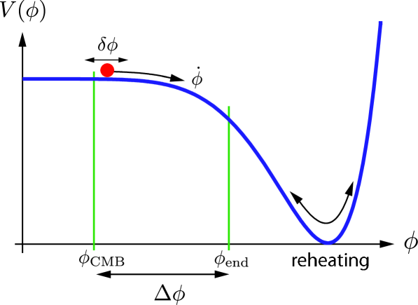
A toy model is shown in Fig. 1. In the slow-roll phase, rolls down on slowly, satisfying Eq. (4) and hence driving the universe to expand exponentially. Near the minima of the potential, oscillates rapidly and inflation ends. After inflation ends, interactions of with other particles lead to decay with a decay rate of , producing particles and radiation. This is called a reheating phase of the universe, as converts its energy density into heat by the particle production.
Not only inflation solves the flatness, homogeneity and isotropy problem, it also gives a mechanism for generating seed perturbations. During inflation the quantum fluctuation in the field are exponentially stretched due to the rapid expansion phase. The proper wavelength of the fluctuations are stretched out of the Hubble-horizon scale to that time, . Once outside the horizon, the characteristic r.m.s. amplitude of these fluctuations is . These fluctuations do not change in time while outside the horizon. After inflation, and reheating, the standard hot-big scenario starts. As the universe decelerates, at some point the fluctuations re-enter the Hubble horizon, seeding matter and radiation fluctuations in the universe. Figure 2 summarizes the evolution of characteristic length scales.
Primordial Perturbations
We use linearly perturbed conformal Friedmann Lemaître Robertson Walker (FLRW) metric of the form,
| (6) |
where all the metric perturbations, , , , and , are , and functions of conformal time . The spatial coordinate dependence of the perturbations is described by the scalar harmonic eigenfunctions, , , and , that satisfy , , and . Note that is traceless: .
Lets consider two new perturbation variables Mukhanov et al. (1992b); Bardeen et al. (1983),
| (7) |
and
| (8) |
which are Gauge invariant. Here , is perturbations in the intrinsic spatial curvature. While reduces to in the spatially flat gauge (), or to in the comoving gauge (), its value is invariant under any gauge transformation. Similarly , which reduces to in the comoving gauge, and to in the spatially flat gauge, is also gauge invariant. The perturbation variable helps the perturbation analysis not only because of being gauge invariant, but also because it is conserved on super-horizon scales throughout the cosmic evolution.
The quantum fluctuations generate the gauge-invariant perturbation, , that reduces to either or depending on which gauge we use, either the spatially flat gauge or the comoving gauge. Hence, and are equivalent to each other at linear order. The benefit of using is that it relates these two variables unambiguously, simplifying the transformation between and .
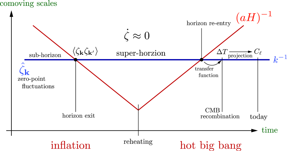
The solution for is valid throughout the cosmic history regardless of whether a scalar field, radiation, or matter dominates the universe; thus, once created and leaving the Hubble horizon during inflation, remains constant in time throughout the subsequent cosmic evolution until reentering the horizon. The amplitude of is fixed by the quantum-fluctuation amplitude in
| (9) |
This is the spectrum of on super-horizon scales.
From Primordial Perturbations to CMB Anisotropies
The metric perturbations perturb CMB, producing the CMB anisotropy on the sky. Among the metric perturbation variables, the curvature perturbations play a central role in producing the CMB anisotropy.
As we have shown in the previous subsection, the gauge-invariant perturbation, , does not change in time on super-horizon scales throughout the cosmic evolution regardless of whether a scalar field, radiation, or matter dominates the universe. The intrinsic spatial curvature perturbation, , however, does change when equation of state of the universe, , changes. Since remains constant, it is useful to write the evolution of in terms of and ; however, is not gauge invariant itself, but is gauge invariant, so that the relation between and may look misleading. In 1980, Bardeen Bardeen (1980) introduced another gauge-invariant variable, (or in the original notation), which reduces to in the zero-shear gauge, or the Newtonian gauge, in which . is given by
| (10) |
Here, the terms in the parenthesis represent the shear, or the anisotropic expansion rate, of the hypersurfaces. While represents the curvature perturbations in the zero-shear gauge, it also represents the shear in the spatially flat gauge in which . Using , we may write as
| (11) |
where the terms in the parenthesis represent the gauge-invariant fluid velocity.
We use in rest of the paper because it gives the closest analogy to the Newtonian potential, which we have some intuition of. reduces to in the zero-shear gauge (or the Newtonian gauge) in which the metric (Eq.(6)) becomes just like the Newtonian limit of the general relativity.
The gauge-invariant velocity term, , differentiates from . Since this velocity term depends on the equation of state of the universe, , the velocity and change as changes, while is independent of . The evolution of on super-horizon scales in cosmological linear perturbation theory gives the following (Kodama and Sasaki, 1984),
| (12) |
for adiabatic fluctuations, and hence in the radiation era (), and in the matter era (). then perturbs CMB through the so-called (static) Sachs–Wolfe effect (Sachs and Wolfe, 1967)
| (13) |
At the decoupling epoch, the universe has already been in the matter era in which , so that we observe adiabatic temperature fluctuations of , and the CMB fluctuation spectrum of the Sachs–Wolfe effect, , is
| (14) |
By projecting the 3-dimension CMB fluctuation spectrum, , on the sky, we obtain the angular power spectrum222For the scale invariant () case, ., (Bond and Efstathiou, 1987),
| (15) |
where and denote the conformal time at the present epoch and at the decoupling epoch, respectively, and is a spectral index which is conventionally used in the literature.
On small angular scales (), the Sachs–Wolfe approximation breaks down, and the acoustic physics in the photon-baryon fluid system modifies the primordial radiation spectrum (Peebles and Yu, 1970). To calculate the anisotropies at all the scales, one has to solve the Boltzmann photon transfer equation together with the Einstein equations. These equations can be solved numerically with the Boltzmann code such as CMBFAST (Seljak and Zaldarriaga, 1996). The CMB power spectrum then can be written as
| (16) |
Here is called the radiation transfer function, and it contains all the physics which modifies the primordial power spectrum to generate CMB power spectrum . For the adiabatic initial conditions, in the Sachs–Wolfe limit, . Often in the literature power spectrum, , is used instead of . The two are related as . is called the dimensionless power spectrum.
If were exactly Gaussian, all the statistical properties of would be encoded in the two-point function or in in the spherical harmonic space. Since is directly related to through Eq. (12), all the information of is also in-coded in . Although which is related to a Gaussian variable, , through , in the linear order also obeys Gaussian statistics; however the non-linear relation between and makes (and hence and CMB anisotropies) slightly non-Gaussian. The non-linear relation between and is not the only source of non-Gaussianity in the CMB anisotropies. For example, at the second order, the relationship between and is also non-linear.
Probes of the Cosmological Initial Conditions
The main predictions of a canonical inflation model are:
-
•
spatial flatness of the observable universe,
-
•
homogeneity and isotropy on large angular scales of the observable universe,
-
•
seed scalar and tensor perturbation with primordial density perturbations being
(a) nearly scale invariant,
(b) nearly adiabatic, and
(c) very close to Gaussian.
At the time of writing, these predictions are consistent with all current observations. This represents a major success for the inflationary paradigm. On the other hand, the inflationary paradigm can be realized by a large ‘zoo’ 333Example of some inflationary models are: eternal inflation, hybrid inflation, chaotic, Ghost inflation, Tilted Ghost inflation, DBI inflation, brane inflation, N-flation, bubble inflation, extended inflation, false vacuum inflation, power law inflation, k-inflation, hyperextended inflation, supersymmetric inflation, Quintessential inflation, Natural inflation, Super inflation, Supernatural inflation, D-term inflation, B -inflation, Thermal inflation, discrete inflation, Assisted inflation, Polar cap inflation, Open inflation, Topological inflation, Double inflation, Multiple inflation, Induced-gravity inflation, Warm inflation, stochastic inflation, Generalized assisted inflation, self-sustained inflation, Graduated inflation, Local inflation, Singular inflation, Slinky inflation, locked inflation, Elastic inflation, Mixed inflation, Phantom inflation, Boundary inflation, Non-commutative inflation, Tachyonic inflation, Tsunami inflation, Lambda inflation, Steep inflation, Oscillating inflation, Mutated Hybrid inflation, intermediate inflation, Inhomogeneous inflation. of models. In addition, somewhat surprisingly, there exist scenarios where the Universe first contracts and then expands (such as the ekpyrotic/cyclic model), which (up to theoretical uncertainties regarding the precise mechanics of the bounce) also reproduce Universes with the properties described above. What we would like to do is to find observables that allows us to distinguish between members of the inflationary zoo. The exciting fact is that upcoming experiments will have the sensitivity to achieve this goal. Tilt and Running: Inflationary models very generically predict a slight deviation from completely flat spectrum. If we write the primordial power spectrum as , then correspond to flat spectrum and the quantity is called a tilt, which characterizes the deviation from scale invariant spectrum. Although the deviations from the scale invariance are predicted to be small, the exact amount of deviation depends on the details of the inflationary model. For example in most slow roll models is of order , where is a number of e-folds to the end of inflation. Ghost inflation, however, predicts negligible tilt. Hence characterizing the tilt of the scalar spectral index is a useful probe of the early universe. Currently the most stringent constraints on tilt come from the WMAP 5-year data, Komatsu et al. (2008), which already disfavors inflationary models with ’blue spectral index’ (). The error on will reduce to for upcoming Planck satellite and to for futuristic CMBPol like satellite Baumann et al. (2009).
Apart from the tilt in the primordial power spectrum, inflationary models also predict to be slightly scale dependent. This scale dependence is referred to as ‘running’ of the spectral index , and is defined as . The constraints on the running from the WMAP 5-year data are Komatsu et al. (2008). The error will reduce to for upcoming Planck satellite and to for a fourth-generation satellite such as CMBPol Baumann et al. (2009).
Primordial Gravitational Waves: Inflation also generates tensor perturbations (gravitational waves), which although small compared to scalar component, are still detectable, in principle. So far primordial gravitational waves have not been detected. There are upper limits on their amplitude; see Ref. Collaboration, The LIGO Scientific and Collaboration, the Virgo (2009) for a current observational bounds on the level for primordial gravitational waves. Detection of these tensor perturbations or primordial gravitational waves is considered a ‘smoking gun’ for the inflationary scenario. In contrast to inflation, ekpyrotic (cyclic) models predict an amount of gravitational waves that is much smaller than polarized foreground emission would allow us to see even for an ideal CMB experiment. Primordial scalar perturbations create only E-modes of the CMB444To first order in perturbations, primordial scalar perturbations do not generate B-modes of CMB. However at second (and higher) order in perturbations, scalar perturbations do produce B-modes Bartolo et al. (2007); Baumann et al. (2007). The B-modes generated from higher order perturbations are expected to be smaller than the tensor B-mode levels that the upcoming and future experiments (like CMBPol) are sensitive too., while primordial tensor perturbations generate both parity even E-modes and parity odd B-modes polarization Seljak and Zaldarriaga (1997); Kamionkowski et al. (1997a, b). The detection of primordial tensor B-modes in the CMB would confirm the existence of tensor perturbations in the early universe. This primordial B-mode signal is directly related to the Hubble parameter during inflation, and thus a detection would establish the energy scale at which inflation happened. Various observational efforts are underway to detect such B-mode signal of the CMB ACTPol , BICEP, CAPMAP, CBI, Clover, CMBPol, EBEX, POLARBEAR, PIPER, PIQUE, QUaD, QUIET, SPIDER (current and upcomming experimets). Search for primordial B-modes is challenging. Apart from foreground subtraction challenges, and the challenge of reaching the instrumental sensitivity to detect primordial B-modes, there are several non-primordial sources such as weak lensing of CMB by the large scale structure Seljak (1996); Zaldarriaga and Seljak (1998), rotation of the CMB polarization Lue et al. (1999); Kamionkowski (2009); Yadav et al. (2009); Gluscevic et al. (2009), and instrumental systematics that generate B-modes which contaminate the inflationary signal Hu et al. (2003); Shimon et al. (2008); Yadav et al. (2009). The amplitude of gravitational waves is parametrized as the ratio of the amplitude of tensor and scalar perturbations, . The limit from WMAP 5-year data is () Komatsu et al. (2008).
Isocurvature Modes: Inflationary models with a single scalar field predict primordial perturbations to be adiabatic. Hence detection of isocurvature density perturbations is a ”smoking gun” for multi-field models of inflation. A large number of inflationary models with multiple scalar fields predict some amount of isocurvature modes Linde A. D. (1984); Kofman L. A. and Linde A. D. (1987); Polarski, David and Starobinsky, Alexei A. (1994); Gordon, Christopher and Wands, David and Bassett, Bruce A. and Maartens, Roy (2001); Linde A. D. (1985); Efstathiou G. and Bond J. R. (1986); Peebles P. J. E. (1987); Kodama H. and Sasaki M. (1986); Weinberg S. (2004); Garcia-Bellido, Juan and Wands, David (1996); Sasaki, Misao and Stewart, Ewan D. (1996); Sasaki and Tanaka (1998); Bartolo et al. (2001). For example, curvaton models predict the primordial perturbations to be a mixture of adiabatic and isocurvature perturbations. Isocurvature initial conditions specify perturbations in the energy densities of two (or more) species that add up to zero. It does not perturb the spatial curvature of comoving slice (i.e is zero, hence the name isocurvature). In general, there can be four types of isocurvature modes, namely: baryon isocurvature modes, CDM isocurvature modes, neutrino density isocurvature modes and, neutrino velocity isocurvature modes. These perturbations imprint distinct signatures in the CMB temperature and E-polarization anisotropies Bucher et al. (2002). The contribution of isocurvature modes is model dependent, and different models predict different amounts of it. There exists an upper limit on the allowed isocurvature modes using CMB temperature anisotropies Bucher et al. (2001); Bean et al. (2006), a characterization (or detection of any) of isocurvature modes has a potential of discriminating between early Universe models.
Primordial Non-Gaussianity: Canonical inflationary models predict primordials perturbations to be very close to Gaussian Guth and Pi (1982); Starobinsky (1982); Hawking (1982); Bardeen et al. (1983); Mukhanov et al. (1992a), and any non-Gaussianity predicted by the canonical inflation models is very small Acquaviva et al. (2003); Maldacena (2003a). However models with non-linearity Salopek and Bond (1990); Gangui et al. (1994); Gupta et al. (2002), interacting scalar fields Allen et al. (1987); Falk et al. (1993), and deviation from ground state Lesgourgues et al. (1997); Martin et al. (2000) can generate large non-Gaussian perturbations. The amplitude of the non-Gaussian contribution to the perturbation is often referred to as even if the nature of the non-Gaussianities can be quite different. Different models of inflation predict different amounts of , starting from very close to zero for almost Gaussian perturbations, to for large non-Gaussian perturbations. For example, the canonical inflation models with slow roll inflation, where only a couple of derivatives of potential are responsible for inflationary dynamics, predict Maldacena (2003a). In models where higher order derivatives of the potential are important, the value of varies from where higher order derivatives are suppressed by a low UV cutoff Creminelli (2003) to based on Dirac-Born-Infeld effective action. Ghost inflation, where during inflation, the background has a constant rate of change as opposed to the constant background in conventional inflation, is also capable of giving Arkani-Hamed et al. (2004). The additional field models generating inhomogeneities in non-thermal species Dvali et al. (2003) can generate Zaldarriaga (2004); while curvaton models, where isocurvature perturbations in second field during the inflation generate adiabatic perturbations after the inflation, can have Lyth et al. (2003).
In the following we will see that non-Gaussianity, far from being merely a test of standard inflation, may reveal detailed information about the state and physics of the very early Universe, if it is present at the level suggested by the theoretical arguments above.
III Primordial Non-Gaussianity
Large primordial non-Gaussianity can be generated if any of the following condition is violated Komatsu et al. (2009)
-
•
Single Field. Only one scalar field is responsible for driving the inflation and the quantum fluctuations in the same field is responsible for generating the seed classical perturbations.
-
•
Canonical Kinetic Energy. The kinetic energy of the field is such that the perturbations travel at the speed of light.
-
•
Slow Roll. During inflation phase the field evolves much slowly than the Hubble time during inflation.
-
•
Initial Vacuum State. The quantum field was in the Bunch-Davies vacuum state before the quantum fluctuation were generated.
To characterize the non-Gaussianity one has to consider the higher order moments beyond two-point function, which contains all the information for Gaussian perturbations. The 3-point function which is zero for Gaussian perturbations contains the information about non-Gaussianity. The 3-point correlation function of Bardeen’s curvature perturbations, , can be simplified using the translational symmetry to give
| (17) |
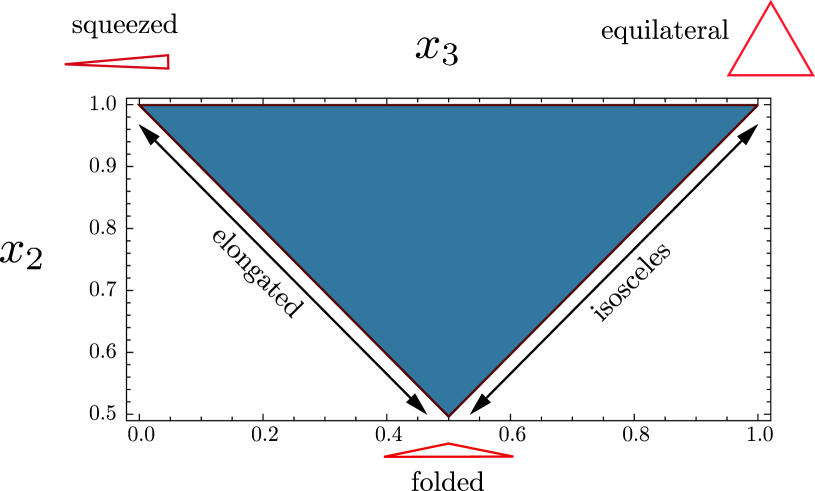
where tells the shape of the bispectrum in momentum space while the amplitude of non-Gaussianity is captured dimensionless non-linearity parameter . The shape function correlates fluctuations with three wave-vectors and form a triangle in Fourier space. Depending on the physical mechanism responsible for the bispectrum, the shape of the 3-point function, can be broadly classified into three classes (Babich et al., 2004). The local, “squeezed,” non-Gaussianity where is large for the configurations in which . Most of the studied inflationary and Ekpyrotic models produce non-Gaussianity of local shape (eg. Bartolo et al. (2002); Bernardeau and Uzan (2002, 2003); Sasaki (2008); Naruko and Sasaki (2009); Byrnes et al. (2008); Byrnes and Wands (2006); Langlois et al. (2008); Valiviita et al. (2008); Assadullahi et al. (2007); Valiviita et al. (2006); Vernizzi and Wands (2006); Allen et al. (2006); Linde and Mukhanov (1997); Dvali et al. (2003); Lyth et al. (2003); Kofman (2003); Lehners and Steinhardt (2008a, b); Koyama et al. (2007)). Second, the non-local, “equilateral,” non-Gaussianity where is large for the configuration when . Finally the folded Holman and Tolley (2008); Chen et al. (2007) shape where is large for the configurations in which . Figure 3 shows these three shapes.
Non-Gaussianity of Local Type: The local form of non-Gaussianity may be parametrized in real space as555Or equivalently Gangui et al. (1994); Verde et al. (2000); Komatsu and Spergel (2001):
| (18) |
where is the linear Gaussian part of the perturbations, and characterizes the amplitude of primordial non-Gaussianity. Different inflationary models predict different amounts of , starting from to , beyond which values have been excluded by the Cosmic Microwave Background (CMB) bispectrum of WMAP temperature data. The bispectrum in this model can be written as
| (19) |
where is the amplitude of the primordial power spectrum.
The local form arises from a non-linear relation between inflaton and curvature perturbations Salopek and Bond (1990, 1991); Gangui et al. (1994), curvaton models Lyth et al. (2003), or the New Ekpyrotic models Koyama et al. (2007); Buchbinder et al. (2007). Models with fluctuations in the reheating efficiency [9, 10] and multi-field inflationary models [17] also generate non-Gaussianity of local type.
Being local in real space, non-Gaussianity of local type describes correlations among Fourier modes of very different . In the limit in which one of the modes becomes of very long wavelength Maldacena (2003b), , (i.e. the other two ’s become equal and opposite), freezes out much before and and behaves as a background for their evolution. In this limit is proportional to the power spectrum of the short and long wavelength modes
| (20) |
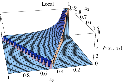
As an example, for canonical single field slow-roll inflationary models, the three point function is given by Maldacena (2003a)
| (21) |
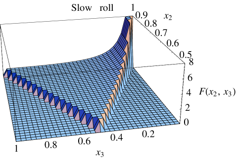
where and are the usual slow-roll parameters and are assumed to be much smaller than unity. Taking the limit gives the local form as in Eq. (20). To show this point, Figure. 4 compares the non-Gaussianity shape for local type and for slow-roll model. Although in this limit, slow-roll models do predict no-Gaussianity of local type but as evident from Eq. (21), the bispectrum of inflaton perturbations yields a non-trivial scale dependence of Falk et al. (1993); Maldacena (2003a). However in the slow roll limit and hence the amplitude is too small to detect.
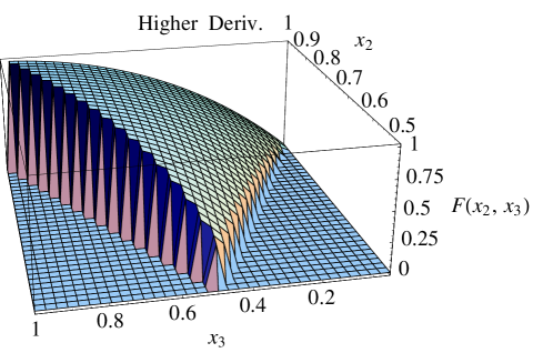
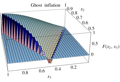
Non-Gaussianity of equilateral type: While vast number of inflationary models predict non-Gaussianity of local type, this model, for instance, fails completely when non-Gaussianity is localized in a specific range in space, the case that is predicted from inflation models with higher derivative kinetic terms Creminelli (2003); Alishahiha et al. (2004); Arkani-Hamed et al. (2004); Seery and Lidsey (2005); Chen et al. (2007); Cheung et al. (2007). In these models the correlation is among modes with comparable wavelengths which go out of the horizon nearly at the same time. The shape function for the equilateral shape can be written as Creminelli et al. (2006)
| (22) | |||||
The models of this kind have large for the configurations where . The equilateral form arises from non-canonical kinetic terms such as the Dirac-Born-Infeld (DBI) action Alishahiha et al. (2004), the ghost condensation Arkani-Hamed et al. (2004), or any other single-field models in which the scalar field acquires a low speed of sound Chen et al. (2007); Cheung et al. (2007).
As an example, models with higher derivative operators in the usual inflation scenario and a model of inflation based on the Dirac-Born-Infeld (DBI) action produce a bispectrum of the form
| (23) |
The above model uses as a leading order operator. DBI inflation, which can produce large non-Gaussianity, , also has of a similar form.
Ghost inflation, where an inflationary de Sitter phase is obtained with a ghost condensate, produces a bispectrum of the following form Arkani-Hamed et al. (2004)
| (24) | ||||
where and are free parameters of order unity, and
| (25) |
Ghost inflation also produces large non-Gaussianity, . Figure 5 shows the shape of non-Gaussianity of equilateral type by showing for ghost inflation and for a model with a higher derivative term.
Folded Shape: So far the 3-point functions were calculated assuming the regular Bunch-Davis vacuum state, giving rise to either local or equilateral type non-Gaussianity. However if the bispectrum is calculated by dropping the assumption of Bunch-Davis initial state give rise to bispectrum shape which peaks for the folded shape, , with shape function given as Holman and Tolley (2008); Meerburg et al. (2009); Chen et al. (2007)
| (26) |
where are the Bogoliubov coefficients which encode information about the initial conditions, is the initial conformal time and .
IV The Cosmic Microwave Background Bispectrum
Since the discovery of CMB by Penzias and Wilson in 1965 Penzias and Wilson (1965) and the first detection of CMB temperature anisotropies on large scales by the COBE DMR Smoot et al. (1992), the space satellite WMAP and over a dozens of balloon and ground based experiments have characterized the CMB temperature anisotropies to a high accuracy and over a wide range of angular scales. The space satellite Planck which launched in 2009 will soon characterize the temperature anisotropies to even higher accuracy up to angular scales of . The CMB power spectrum is obtained by reducing all the information of ( for WMAP and for Planck). Such reduction is justified to obtain a fiducial model, given the non-Gaussianities are expected to be small. With high quality data on the way, the field of non-Gaussianity is taking off. CMB bispectrum contains information which is not present in the power-spectrum and as we say in the previous section, is a unique probe of the early universe.
The harmonic coefficients of the CMB anisotropy can be related to the primordial fluctuation as
| (27) |
where is the primordial curvature perturbations, for a comoving wavevector , is the radiation transfer function where the index refers to either temperature () or E-polarization () of the CMB. A beam function and the harmonic coefficient of noise are instrumental effects. Eq. (27) is written for a flat background, but can easily be generalized.
Any non-Gaussianity present in the primordial perturbations gets transferred to the observed CMB via Eq. (27). The most common way to look for non-Gaussianity in the CMB is to study the bispectrum, the three-point function of temperature and polarization anisotropies in harmonic space. The CMB angular bispectrum is defined as
| (28) |
and the angular-averaged bispectrum is
| (29) |
where the matrix is the Wigner 3J symbol imposing selection rules which makes bispectrum zero unless
(i) integer
(ii)
(iii) for .
Using Eq.(27) the bispectrum can be written as
| (33) | |||||
where is the primordial curvature three-point function as defined in Eq. (17).
To forecast constraints on non-Gaussianity using CMB data, we will perform a Fisher matrix analysis. The Fisher matrix for the parameters can be written as Komatsu and Spergel (2001); Babich and Zaldarriaga (2004); Yadav et al. (2008)
| (34) |
The indices and run over all the parameters bispectrum depends on, we will assume all the cosmological parameters except to be known. Indices and run over all the eight possible ordered combinations of temperature and polarization given by , , , , , , and ; the combinatorial factor equals when all ’s are different, when , and otherwise. The covariance matrix Cov is obtained in terms of , , and (see Babich and Zaldarriaga (2004); Yadav et al. (2007)) by applying Wick’s theorem.
For non-Gaussianity of the local type, for which the functional form is given by Eq. (19), we have
| (35) |
where the functions and are given by
| (36) | |||||
| (37) |
In the expression above we use the dimensionless power spectrum amplitude , which is defined by , where is the tilt of the primordial power spectrum. One can compute the transfer functions and using publicly available codes such as CMBfast Seljak and Zaldarriaga (1996) and CAMB Lewis et al. (2000)
In a similar way, from Eq. (22), one can derive the following expressions for the bispectrum derivatives in the equilateral case,
| (41) | |||||
where the functions and are given by
| (42) | |||||
| (43) |
Recently a new bispectrum template shape, an orthogonal shape has been introduced Senatore et al. (2009a) which characterizes the size of the signal () which peaks both for equilateral and flat-triangle configurations. The shape of non-Gaussianities associated with is orthogonal to the one associated to . The bispectrum for orthogonal shape can be written as Senatore et al. (2009a)
| (47) | |||||
IV.1 Estimator
An unbiased bispectrum-based minimum variance estimator for the nonlinearity parameter in the limit of full sky and homogeneous noise can be written as Komatsu et al. (2005); Creminelli et al. (2006); Yadav et al. (2008)
| (50) |
where is angle averaged theoretical CMB bispectrum for the model in consideration. The normalization can be calculated to require the estimator to be unbiased, . If the bispectrum is calculated for then the normalization takes the following form
| (51) |
The estimator for non-Gaussianity, Eq. (50), can be simplified using Eq. (27) to yield
| (52) | |||||
where is a shape of 3-point function as defined in Eq. (17). Given the shape , one is interested in, it is conceptually straightforward to constrain the non-linearity parameter from the CMB data. Unfortunately the computation time for the estimate scales as , which is computationally challenging as even for the WMAP data the number of pixels is of order . The scaling can be understood by noting that the each spherical harmonic transform scales as and the estimator requires number of spherical harmonic transforms.
The computational cost decreases if the shape can be factorized as
| (53) |
with which the estimator simplifies to
| (54) |
and computational cost now scales as . For Planck () this translates into a speed-up by factors of millions, reducing the required computing time from thousands of years to just hours and thus making estimation feasible for future surveys. The speed of the estimator now allows sufficient number of Monte Carlo simulations to characterize its statistical properties in the presence of real world issues such as instrumental effects, partial sky coverage, and foreground contamination. Using the Monte Carlo simulations it has been shown that estimator is indeed optimal, where optimality is defined by saturation of the Cramer Rao bound, if noise is homogeneous. Note that even for the non-factorizable shapes, by using the flat sky approximation and interpolating between the modes, one can estimating in a computationally efficient way Fergusson and Shellard (2009).
The extension of the estimator of from the temperature data Komatsu et al. (2005) to include both the temperature and polarization data of the CMB is discussed in Yadav et al. Babich and Zaldarriaga (2004); Yadav and Wandelt (2005); Yadav et al. (2007, 2008). Summarizing briefly, we construct a cubic statistic as a combination of (appropriately filtered) temperature and polarization maps which is specifically sensitive to the primordial perturbations. This is done by reconstructing a map of primordial perturbations, and using that to define a fast estimator. We also show that this fast estimator is equivalent to the optimal estimator by demonstrating that the inverse of the covariance matrix for the optimal estimator Babich and Zaldarriaga (2004) is the same as the product of inverses we get in the fast estimator. The estimator still takes only operations in comparison to the full bispectrum calculation which takes operations.
For a given shape the estimator for non-linearity parameter can be written as , where for the equilateral, local and orthogonal shapes, the can be written as
| (55) | |||||
| (56) | |||||
| (57) |
with
| (58) |
| (59) |
and is a fraction of sky. Index and can either be or .
| (60) |
Indices and can either be or . Here, is 1 when , 6 when , and 2 otherwise, is the theoretical bispectrum for Yadav et al. (2007).
It has been shown that the above estimators defined in Eq. (57) are minimum variance amongst bispectrum-based estimators for full sky coverage and homogeneous noise Yadav et al. (2007). To be able to deal with the realistic data, the estimator has to be able to deal with the inhomogeneous noise and foreground masks. The estimator can be generalized to deal with partial sky coverage as well as inhomogeneous noise by adding a linear term to : . For the temperature only case, this has been done in Creminelli et al. (2006). Following the same argument, we find that the linear term for the combined analysis of CMB temperature and polarization data is given by
| (61) |
where and are the and maps generated from Monte Carlo simulations that contain signal and noise, and denotes the average over the Monte Carlo simulations.
The generalized estimator is given by
| (62) |
Note that , and this relation also holds for the equilateral shape. Therefore, it is straightforward to find the generalized estimator for the equilateral shape: first, find the cubic estimator of the equilateral shape, , and take the Monte Carlo average, . Let us suppose that contains terms in the form of , where , , and are some filtered maps. Use the Wick’s theorem to re-write the average of a cubic product as . Finally, remove the MC average from single maps, and replace maps in the product with the simulated maps . This operation gives the correct expression for the linear term, both for the local form and the equilateral form.
The main contribution to the linear term comes from the inhomogeneous noise and sky cut. For the temperature only case, most of the contribution to the linear term comes from the inhomogeneous noise, and the partial sky coverage does not contribute much to the linear term. This is because the sky-cut induces a monopole contribution outside the mask. In the analysis one subtracts the monopole from outside the mask before measuring , which makes the linear contribution from the mask small Creminelli et al. (2006). For a combined analysis of the temperature and polarization maps, however, the linear term does get a significant contribution from a partial sky coverage. Subtraction of the monopole outside of the mask is of no help for polarization, as the monopole does not exist in the polarization maps by definition. (The lowest relevant multipole for polarization is .)
The estimator is still computationally efficient, taking only (times the sampling, which is of order 100) operations in comparison to the full bispectrum calculation which takes operations. Here refers to the total number of pixels. For Planck, , and so the full bispectrum analysis is not feasible while our analysis is.
V Constraints from the CMB Bispectrum
V.1 Current Status
Currently the the Wilkinson Microwave Anisotropy Probe (WMAP) satellite provides the “best” (largest number of signal dominated modes) CMB data for non-Gaussianity analysis. Over the course of WMAP operation the field of non-Gaussianity has made vast progress both in terms of theoretical predictions of non-Gaussianities from inflation and improvement in the bispectrum based estimators. At the time of WMAP’s first data release in 2003 the estimator was sub-optimal in the presence of partial sky coverage and/or inhomogeneous noise. With the sub-optimal estimator one could not use the entirety of WMAP data and only the data up to were used to obtain the constraint Komatsu et al. (2003). These limits were around 30 times better than the previous constraints of from the Cosmic Background Explorer (COBE) satellite fnl_cobe.
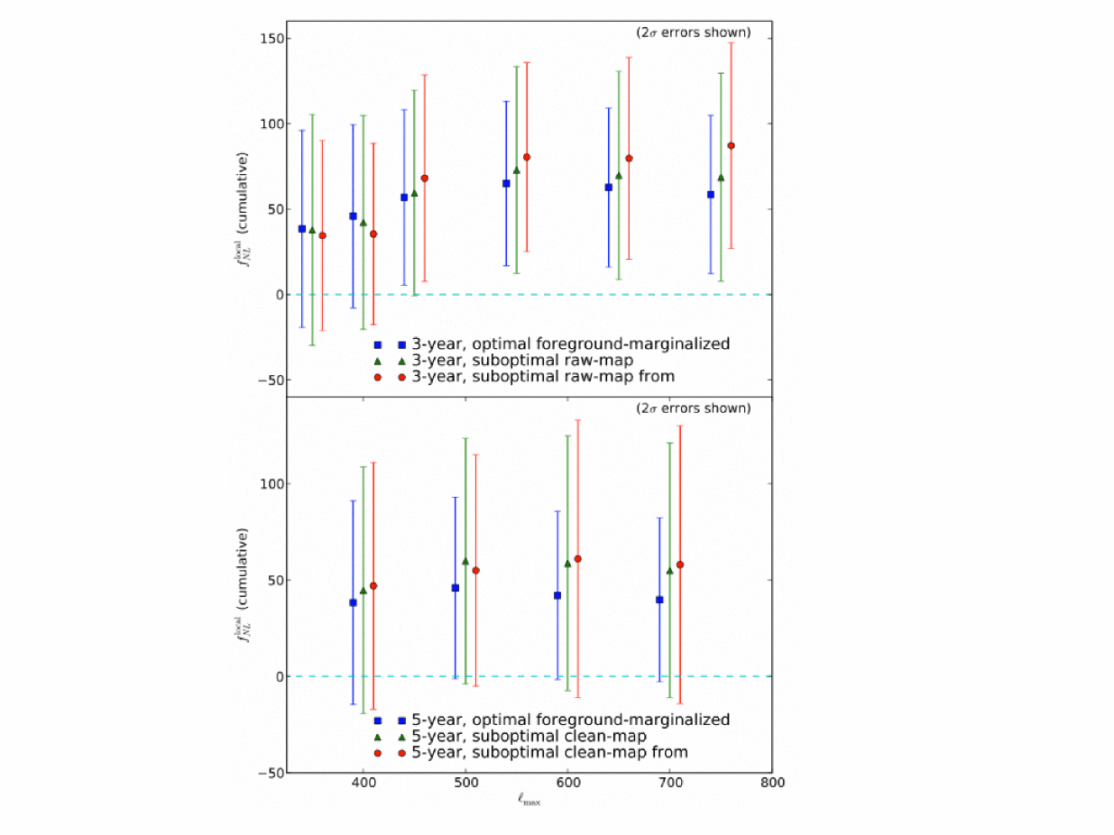
By the time of second WMAP release in 2007 the estimator was generalized by adding a linear to the KSW estimator which allows to deal with partial sky coverage and inhomogeneous noise. The idea of adding a linear term to reduce excess variance due to noise inhomogeneity was introduced in Creminelli et al. (2006). Applied to a combination of the Q, V and W channels of the WMAP 3-year data up to this estimator had yielded the tightest constraint at the time on as: Creminelli et al. (2007a). This estimator was further generalized to utilize both the temperature and E-polarization information in Yadav et al. (2008), where it was pointed out that the linear term had been incorrectly implemented in Eq. 30 of Creminelli et al. (2006). Using Monte-Carlo simulations it has been shown that this corrected estimator is nearly optimal and enables analysis of the entire WMAP data without suffering from a blow-up in the variance at high multipoles666We will refer to the estimator in Ref. Creminelli et al. (2006) as a near-optimal-v1, while the corrected estimator of Ref. Yadav and Wandelt (2008) as near-optimal.. The first analysis using this estimator shows an evidence of non-Gaussianity of local type at around in the WMAP 3-year data. Independent analysis shows the evidence of non-Gaussianity at lower significance, around (see Table 2).
By the time of the third WMAP data release (with 5-year obsevational data) in 2008 the estimation technique was improved further by implementing the covariance matrix including inhomogeneoous noise to make the estimator completely optimal Smith et al. (2009). Using the optimal estimator and using the entirety of WMAP 3-year data there is an evidence for non-Gaussianity of local type at around level Smith et al. (2009). However with WMAP 5-year data the significance goes down from to Smith et al. (2009). Table 2 compares the constraints obtained by different groups using WMAP 3-year and WMAP 5-year data. Fig 6 shows this comparison in more detail, showing the constraints also as a function of maximum multipole used in the analysis. Few comments are in place: 1) constraints on from WMAP 3-year data as a function of show a trend where the mean value rises at around , below which data is consistent with Gaussianity and above which there is deviation from Gaussianity at above . The result becomes roughly independent of with evidence for non-Gaussianity at around level, 2) independent analysis and using different estimators (optimal and near-optimal with linear term) sees this deviation from non-Gaussianity at around in WMAP 3-year data, 3) significance of non-Gaussianity goes down to around with WMAP 5-year data. The drop in the mean value between WMAP 3-year and 5-year data can be attributed to statistical shift.
The best constraints on the equilateral and orthogonal shape of non-Gaussianity using the WMAP 5-year data are and respectively Senatore et al. (2009a).
As we were completing this article, the WMAP 7-year data was released, with constraints and Komatsu et al. (2010).
V.2 Future Prospects
Now we discuss the future prospects of using the bispectrum estimators for constraining the non-linearity parameter for local and equilateral shapes. We compute the Fisher bounds for three experimental setups, (1) cosmic variance limited experiment with perfect beam (ideal experiment hereafter), (2) Planck satellite with and noise sensitivity K-arcmin and beam FWHM (3) a futuristic CMBPol like satellite experiment with noise sensitivity K-arcmin and beam FWHM (CMBPol hereafter). Beside we fix all the other cosmological parameters to a standard fiducial model with a flat cosmology, with parameters described by the best fit to WMAP 5-year results Komatsu et al. (2008), given by and . We calculate the theoretical CMB transfer functions and power spectrum from publicly available code CMBFAST Seljak and Zaldarriaga (1996). We also neglect any non-Gaussianity which can be generated during recombination or there after. We discuss the importance and effect of these non-primordial non-Gaussianities in next section.
The scaling of signal-to-noise as a maximum multipole for the local Creminelli et al. (2007b); Liguori et al. (2007) and equilateral model Bartolo and Riotto (2009) are
| (63) |
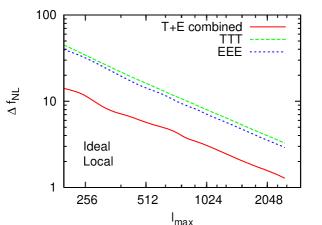
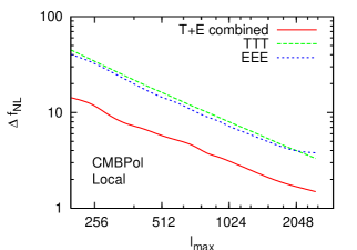
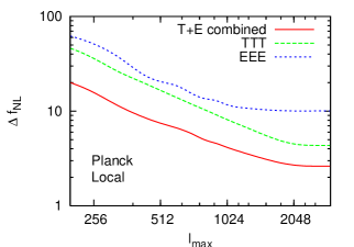
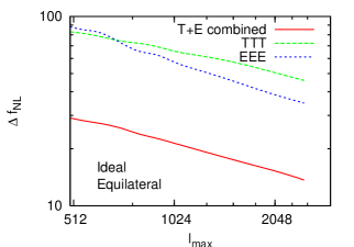
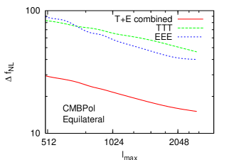
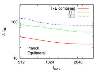
In principle one could go to arbitrary high but in reality secondary signals will certainly overwhelm primary signal beyond , we restrict to the analysis to . In Figure 7 we show the Fisher bound as function of maximum multipole , for local and equilateral type of non-Gaussianity. For both local and equilateral case we show the Fisher bound for the analysis using only the CMB temperature information (TTT), only the CMB polarization information (EEE), and the combined temperature and polarization analysis. Note that by having both the temperature and -polarization information one can improve the sensitivity by combining the information. Apart from combining the T and E signal, one can also do cross-checks and diagnostics by independently analysing the data. Temperature and polarization will have different foregrounds and instrumental systematics.
A CMBPol like experiment will be able to achieve the sensitivity of for non-Gaussianity of local type and for non-Gaussianity of equilateral type. For the local type of non-Gaussianity this amounts to an improvement of about a factor of 2 over the Planck satellite and about a factor of 12 over current best constraints. These estimates assume that foreground cleaning can be done perfectly, i.e. the effect of residual foregrounds has been neglected. Also the contribution from unresolved point sources and secondary anisotropies such as ISW-lensing and SZ-lensing has been ignored.
| data (mask, estimator) | error | deviation from Gaussianity | |
| WMAP 3-year (Kp0, near-optimal) | Yadav and Wandelt Yadav and Wandelt (2008) | ||
| WMAP 3-year (KQ75, optimal) | Smith et al. Smith et al. (2009) | ||
| WMAP 3-year (Kp0, near-optimal) | Smith et al. Smith et al. (2009) | ||
| WMAP 5-year (KQ75, near-optimal) | Komatsu et al. Komatsu et al. (2008) | ||
| WMAP 5-year (KQ75, optimal) | Smith et al. Smith et al. (2009) |
Running non-Gaussianity: The primordial non-Gaussian parameter has been shown to be scale-dependent in several models of inflation with a variable speed of sound, such as Dirac-Born-Infeld (DBI) models. Starting from a simple ansatz for a scale-dependent amplitude of the primordial curvature bispectrum for primordial non-Gaussianity,
| (64) |
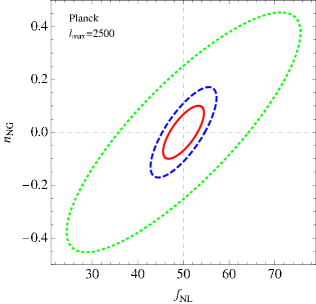
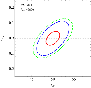
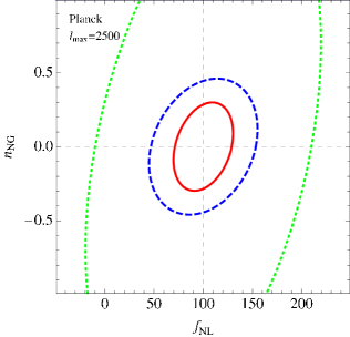
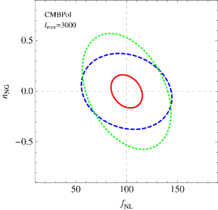
where and is a pivot point. The primordial bispectrum is therefore determined in terms of two parameters: the amplitude and the new parameter quantifying its running. One can generalize the Fisher matrix analysis of the bispectra of the temperature and polarization of the CMB radiation and derive the expected constraints on the parameter that quantifies the running of for current and future CMB missions such as WMAP, Planck and CMBPol. We will consider some non-zero as our fiducial value for the Fisher matrix evaluation. Clearly, in order to be able to constrain a scale-dependence of , its amplitude must be large enough to produce a detection. If is too small to be detected ( is a lowest theoretical limit even for the ideal experiment), we will obviously not be able to measure any of its features, either. In the following we will then always consider a fiducial value of large enough to enable a detection. Figure 8 shows the joint constraints on and . In the event of a significant detection of the non- Gaussian component, corresponding to for the local model and for the equilateral model of non-Gaussianity, is able to determine with a uncertainty of and , respectively, for the Planck mission and a factor of two better for CMBPol. In addition to CMB one can include the information of the galaxy power spectrum, galaxy bispectrum, and cluster number counts as a probe of non- Gaussianity on small scales to further constrain the two parameters Sefusatti et al. (2009).
V.3 Contaminations
A detection of non-Gaussianity has profound implications on our understanding of the early Universe. Hence it is important to know and quantify all the possible sources of non-Gaussianities in the CMB. Here we highlight some sources of non-Gaussianities due to second-order anisotropies after last scattering surface and during recombination. The fact that Gaussian initial conditions imply Gaussianity of the CMB is only true at linear order. We will also discuss the effects of instrumental effects and uncertainties in the cosmological parameters on the bispectrum estimate.
Secondary non-Gaussianities
Current analysis of the CMB data ignore the contributions from the secondary non-Gaussianities. For WMAP resolution it may not be a bad approximation. Studies of the dominant secondary anisotropies conclude that they are negligible for the analysis of the WMAP data for Komatsu and Spergel (2001); Serra and Cooray (2008). However on smaller angular scales several effects starts to kick in, for example, 1) the bispectrum contribution due to unresolved point source like thermal Sunyaev-Zeldovich clusters or standard radio sources, 2) three way correlations between primary CMB, lensed CMB and secondary anisotropies. We will refer to the bispectrum generated due to this three way correlation as , where some secondaries are, the integrated Sachs-Wolfe (ISW) , Sunyaev-Zeldovich signal and Rees-Sciama Goldberg and Spergel (1999); Spergel and Goldberg (1999); Cooray and Hu (2000); Komatsu and Spergel (2001); Komatsu et al. (2003); Serra and Cooray (2008).
For Future experiments such as Planck and CMBPOl the joint estimation of primordial and secondary bispectrum will be required. The observed bispectrum in general would take the following form
| (65) |
The amplitude of bispectrum due to primary-lensing-secondary cross-correlation is proportional to the product of primary CMB power-spectrum and power spectrum of cross-correlation between secondary and lensing signal.
The reduced bispectrum from the residual point sources (assuming Poisson distributed) is constant i.e. The value of the constant will depend on the flux limit at which the point source can be detected and on assumed flux and frequency distribution of the sources.
Depending on the shape of primordial bispectrum in consideration, some secondary bispectra are more dangerous than others. For example, ISW-lensing peaks at the “local” configurations, hence is more dangerous for local primordial shape than the equilateral primordial shape. For example for the Planck satellite if the secondary bispectrum is not incorporated in the analysis, the ISW-lensing contribution will bias the estimate for the local by around Smith and Zaldarriaga (2006b). The bispectrum contribution from primary-lensing-Rees-Sciama signal also peaks at squeezed limit and contribute to effective local Mangilli and Verde (2009). For Planck sensitivity the point source will contamination the local non-Gaussianity by around Babich and Pierpaoli (2008). A recent analysis of the full second order Boltzmann equation for photons Pitrou et al. (2010) claims that second order effects add a contamination .
The generalization of the Fisher matrix given by Eq. (34) to include multiple bispectrum contribution is
| (66) |
where the additional and indices denote a component such as primordial, point-sources, ISW-lensing etc. For fixed cosmological parameters, the signal-to-noise for the component is
| (67) |
Non-Gaussianities from recombination
Non-Gaussianities can be generated during recombination. One requires to solve second order Boltzmann and Einstein equations to evaluate the effect. The second order effect on CMB is an active field of study Hu et al. (1994); Dodelson and Jubas (1995); Pyne and Carroll (1996); Mollerach and Matarrese (1997); Matarrese et al. (1998); Bartolo et al. (2004b, c); Creminelli and Zaldarriaga (2004); Bartolo et al. (2004); Tomita (2005); Bartolo et al. (2005); Bartolo et al. (2006a); Tomita (2008); Pitrou et al. (2008); Bartolo et al. (2006b); Bartolo et al. (2007); Pitrou (2009); Senatore et al. (2009b); Boubekeur et al. (2009); Khatri and Wandelt (2010a), see Ref. Bartolo et al. (2010) for a recent review. The non-Gaussianities produced during recombination comprise of various effects, for example see Ref. Bartolo et al. (2007).
The dominant bispectrum due to perturbative recombination comes from perturbations in the electron density. The amplitude of perturbations of the free electron density is around a factor of 5 larger than the baryon density perturbations Novosyadlyj (2006). The bispectrum generated due to peaks around the “local” configuration with corresponding effective non-linearity amplitude Khatri and Wandelt (2009); Senatore et al. (2009c); Khatri and Wandelt (2010b).
The bispectrum contribution due to second order terms which are the products of the first order perturbations is calculated in Ref. Nitta et al. (2009). The bispectrum contribution from these terms which also peak for the squeezed triangles is small and can be neglected in the analysis. For example the signal-to-noise is about 0.4 at for a full-sky, cosmic variance limited experiment.
Another contribution to bispectrum which peaks for the equilateral configurations comes from the non-linear evolution of the second order gravitational potential. Because of this effect the minimum detectable non-Gaussianity parameter changes by for Planck like experiment Bartolo and Riotto (2009). The bispectrum peaks for the equilateral shape because the the growth of potential happens on scales smaller than the horizon size.
On large scales, in the absence of primordial non-Gaussianities and assuming matter domination (so that the early and late ISW can be neglected), it has been shown in Ref. Boubekeur et al. (2009) that for the squeezed limit the effective generated by second order gravitational effects on the CMB is (also see Bartolo et al. (2004b, c); Creminelli and Zaldarriaga (2004)). Here is the angle between the short and the long modes. The angle dependent contribution comes from lensing.
Effect of Cosmological parameter uncertainties
Impact of uncertainties on the cosmological parameters effect the error bar on . The effect of cosmological parameters have been discussed in Ref. Creminelli et al. (2006); Creminelli et al. (2007a); Yadav and Wandelt (2008); Liguori and Riotto (2008). The cosmological parameters are determined using the 2-point statistics of the CMB and therefor we expect the largest effect of would come from those parameters which leave the CMB power spectrum unchanged while change the bispectrum. The expectation value of the estimator
| (68) |
changes with the change in cosmological parameters. Here is the true CMB bispectrum. When changing the parameters the normalization should be changed to make the estimator unbiased. In general for a set of cosmological paramerets , the error in is given by Liguori and Riotto (2008)
| (69) |
Here the average parameter values and their covariance matrix can be determined using CMB-likelihood analysis tools.
If the parameters are allowed to vary in the analysis then for WMAP this increases the uncertainty in by for the local shape and for the equilateral shape. For Planck experiment the increases in uncertainity is for local shape and for the equilateral shape. Most of the contribution to the error comes from three cosmological parameters, the amplitude of scalar perturbations , the tilt of the power spectrum of the saclar perturbations , and re-ionization optical depth .
For modes inside the horizon during reionization, the reionization optical depth appears as a multiplicative factor in front of transfer function . For local model one of the mode is outside so the effect on bispectrum and for equilateral model all the modes are inside the horizon so . This reduces to for local model and for equilateral model.
The effect of amplitude of perturbations can be seen by noting that the level of non-Gaussianity is given by . Hence the decrease (increase) in the amplitude of perturbations relax (tighten) the constraints on . The effect of red tilt () can be thought of as a reduction in power on at scales shorter than first peak and enhancement of power on larger scales. The effect of blue tilt is just opposite of red tilt. For local shape the limit on becomes tighter proportional to Creminelli et al. (2007a). Note that Ref. Liguori and Riotto (2008) show that the effect of cosmological parameters is negligible if the parameters are allowed to vary in the analysis and then marginalize over.
Instrumental effects and distortions along the line of sight
Here we point out that any cosmological or instrumental effect that can be modelled as a line of a sight CMB distortions of the primary CMB do not generate new bispectrum contribution. Although they can modify the the primordial bispectrum. A general model of line of sight distortions of the primary CMB are described in Ref. Hu et al. (2003); Su et al. (2009); Yadav et al. (2009) where the changes in the Stokes parameter of the CMB due to distortions along the line-of-sight can be written as
| (70) | |||||
The first line captures the distortions in a single perfectly known direction . The distortions in second line capture mixing of the polarization fields in a local region of length scale around . We Taylor expand the CMB fields and around the point and consider the leading order terms. Here and stands for primordial (un-distorted) CMB fields. Since is spin field, is a scalar field that describes modulation in the amplitude of the fields in a given direction ; is also a scalar field that describes the rotation of the plane of polarization, are spin fields that describe the coupling between two spin states (spin-flip), and are spin fields that describe leakage from the temperature to polarization (monopole leakage hereon). Distortions in the second line of Eqn. (70), , and are measured in the units of the length scale . The field is a spin field and describes the change in the photon direction; we will refer to it as a deflection field. Finally and describe leakage from temperature to polarization, is spin field and we will refer to it as dipole leakage; is a scalar field that we will call quadrupole leakage.
These distortions can be produced by various cosmological processes such as weak gravitational lensing of the CMB, screening effects from patchy reionization, rotation of the plane of polarization due to magnetic fields or parity violating physics and various instrumental systematics such as gain fluctuations, pixel rotation, differential gain, pointing, differential ellipticity are also captured via line of sight distortions. All these distortions modify the primordial bispectrum as
| (71) |
where is a window which depends on the type of distortion in consideration and tells how the primordial CMB bispectrum modes are coupled to the distortion field power spectrum . The effect of the distortions on the bispectrum is to smooth out the acoustic features. These effects for the case of lensing have been shown to be small and can be neglected Hanson et al. (2009); Cooray et al. (2008).
In Ref. Donzelli et al. (2009) the impact of the noise and asymmetric beam on local has been found insignificant in the context of a Planck-like experiment.
VI Other probes of non-Gaussianity in the CMB
Although using the full bispectrum is the most sensitive cubic statistic other statistical methods may be sensitive to different aspects of non-Gaussianity and, more importantly, different methods have different systematic effects. Therefore it is important to study various probes. In this section we will discuss some of the methods which have been recently used or developed to test for primordial non-Gaussianities in the CMB.
Trispectrum
The four-point function in harmonic space is called trispectrum, which can be written as
| (76) |
where is the angular averaged trispectrum, is the length of a diagonal that forms triangles with and and with and , and the matrix is the Wigner 3- symbol. The trispectrum contains unconnected part, ,
| (77) | |||||
which comes from the Gaussian part of the perturbations, and the connected part which contains non-Gaussian signatures. Using permutation symmetry, one may write the connected part of the trispectrum as
| (82) |
where
| (83) |
Here, the matrix is the Wigner 6- symbol, and is called the reduced trispectrum, which contains all the physical information about non-Gaussianities. For non-Gaussianity of local-type for which
| (84) |
both and contribute to the trispectrum, but only contributes to the bispectrum. Tripectrum based estimators for measuring and have been developed Okamoto and Hu (2002); Kogo and Komatsu (2006); Creminelli et al. (2007); Munshi et al. (2009); Regan et al. (2010). For local template, the bispectrum nearly contains all the information on Creminelli et al. (2007), however if the non-Gaussianity is seen in bispectrum, trispectrum can serve as a important cross-check. Generically for single field slow-roll models the trispectrum is small and un-observable Seery et al. (2007) however for more general single field models whenever the equilateral bispectrum is large, the trispectrum is large as well Huang and Shiu (2006); Chen et al. (2009); Arroja et al. (2009). For example for equilateral non-Gaussianity Ref. Engel et al. (2009) study how to tune the model parameters to get large trispectrum and small bispectrum. For multi-field inflation one can construct models that predicts small but large , for example Ref. Byrnes et al. (2006) discusses the local form from a multi-field inflation, and briefly mentioned the condition in their class of models to get the large trispectrum and small bispectrum. Joint constraints on both and have the potential to add to the specificity of the search for primordial non-Gaussianity. For a given model these two numbers will often be predicted in terms of a single model parameter, such as a coupling constant, see e.g. Lehners and Steinhardt (2009) for the case of ekyprotic models. Using WMAP 5-year data, the constraints on using the trispectrum are at Smidt et al. (2010).
Minkowski Functionals
Minkowski Functionals (MFs) describe morphological properties (such as area, circumference, Euler characteristic) of fluctuating fields Mecke et al. (1994); Schmalzing and Buchert (1997); Schmalzing and Gorski (1997); Winitzki and Kosowsky (1998). For a -dimensional fluctuating field, , the -th Minkowski Functionals of weakly non-Gaussian fields in, for a given threshold can be written asMatsubara (1994, 2003)
| (85) | |||||
where is the variance of the fluctuating field, are the Hermite polynomials, , and finally are the “skewness parameters” defined as
| (86) | |||||
| (87) | |||||
| (88) |
which characterize the skewness of fluctuating fields and their derivatives. Here characterizes the variance of the fluctuating field and is given by
| (89) |
For CMB, for which and , the skewness parameters are Hikage et al. (2006)
| (90) | |||||
where is the CMB bispectrum, represents a smoothing kernel which depends on the experiment beam and is the usual Gaunt function.
Since MFs can be determined as weighted sum of the bispectrum, they contain less information than the bispectrum. MFs can still be useful because they perhaps suffer from different systematics, though they are less specific to primordial non-Gaussianity since they measure a smaller number of independent bispectrum modes. Also, the bispectrum is defined in Fourier (or harmonic) space while the MFs are defined in real space. Limits on non-Gaussianity of local-type from the MFs of the WMAP 5-year temperature data are Hikage et al. (2008). The MFs from the Planck temperature data should be sensitive to at level Hikage et al. (2006) in contrast to bispectrum which is sensitive to at level. Note that polarization data further improves the sensitivity.
Wavelets
Several studies have used wavelet representations of the WMAP maps to search for a non-Gaussian signal Aghanim and Forni (1999); Hobson et al. (1999); Vielva et al. (2004); Starck et al. (2004); Jin et al. (2005); Vielva et al. (2006); McEwen et al. (2007). In most of these studies, wavelets were used as a tool for blind searches of non-Gaussian anomalies in a basis with resolution in both scale and location. However, in some more recent studies, wavelets were tuned to look for non-Gaussianity of a particular type. In the context of searches for primordial non-Gaussianity of local type, wavelet based estimators for have been built by extracting a signature of local non-Gaussianity that is cubic in the wavelet coefficients from simulations of non-Gaussian skies and searching for this signature in data. This ability to calibrate on a set of simulations makes the wavelet approach very flexible. While not optimal in a least-squared sense, using a wavelet representation can be thought of as a generalized cubic statistic with a different weighting scheme to the optimal bispectrum estimator. Using such estimators therefore provides a useful exploration of nearly optimal cubic estimators similar to the full bispectrum estimator. Any believable detection of non-Gaussianity should be robust to such changes in the analysis. Similarly, contaminating non-Gaussianity from astrophysical and instrumental systematics will propagate through the analysis in a different way to the bispectrum-based analysis.
There are several constraints on local using wavelet based estimators. For example, using the COBE data the constraints are Cayón et al. (2003). Using an estimator based on the skewness of the wavelet coefficients, Mukherjee and Wang constrain the value for WMAP 1-yr data obtaining Mukherjee and Wang (2004). Using an extension of the previous estimator by combining wavelet coefficients at different contiguous scales, Curto et al. obtain Curto et al. (2009a). Recently, using a generalized third order estimator based on the wavelet coefficients, Curto et al. obtain Curto et al. (2009b).
Needlet Bispectrum
Needlets are a family of spherical wavelets which are localized and asymptotically uncorrelated Narcowich et al. (2006a, b). The needlet based statistics as been considered for testing Gaussianity and isotropy (for example see Ref. Baldi et al. (2008, 2009a, 2009b); Lan and Marinucci (2008); Pietrobon et al. (2009, 2010); Cabella et al. (2010). Using the bispectrum of needlet coefficient, the constraints on non-Gaussianity of local-type using WMAP 5-year data yields Rudjord et al. (2009, 2010). As is clear, the needlet based bispectrum is not as sensitive as the CMB bispectrum discussed in Sec. IV, however again in the event of detection the needlet based methods can be calibrated on simulations and represent a different weighting scheme for handling the sky mask and anisotropic noise. Finally, needlets and wavelets allow for the possibility to analyze spatially localized regions in the sky.
Probing non-Gaussianity using Bayesian statistics
A somewhat different approach to searching for non-Gaussianity is provided by the Bayesian approach. Here, the starting point is an explicit physical or statistical model for the data and the goal is to evaluate the posterior density of the parameters of the model and/or the relative probability of the Gaussianity and non-Gaussianity.
On large scales, in the Sachs-Wolfe regime, one can simplify the Bayesian approach by modeling directly the temperature anisotropy. Rocha et al. (2001) Rocha et al. (2001) discuss a Bayesian exploration of a model where each spherical harmonic coefficient is drawn from a non-Gaussian distribution. In this regime, the simple form of the non-Gaussian potential for the local model Eq. (18) also translates into a simple model for the temperature anisotropy. Ref. Vielva and Sanz (2008) develop several results for it, including an analytical expression of the evidence ratio of the Gaussian and non-Gaussian models. At the level of current data, this approximation is too restrictive, since most of the information about is contained near the resolution limit of the experiment, where most of the measured perturbation modes are concentrated.
A full implementation of a physical non-Gaussian model must include the effect of Boltzmann transport. In the context of local non-Gaussianity, the model equation Eq. (18) suggests that a full Bayesian treatment may be feasible. At the time of writing, no fully Bayesian analysis for local has been published. The effort has focused on developing approximations to the full Bayesian problem.
Using a perturbative analysis, Ref. Enßlin et al. (2009) relate the frequentist bispectrum estimator to moments of the Bayesian posterior distribution. Ref. Elsner et al. (2010) described approximations to the full Bayesian treatment that simplify the analysis for high signal-to-noise maps and compare these to the full Bayesian treatment for a simple 1-D toy model of non-Gaussian sky where this analysis is feasible.
| Year | data | Method | error | |
|---|---|---|---|---|
| 2002 | COBE | Bispectrum sub-optimal | Komatsu et al. Komatsu et al. (2002) | |
| 2003 | MAXIMA | Bispectrum sub-optimal | Santos et al. Santos et al. (2003) | |
| 2003 | WMAP 1-year | Bispectrum sub-optimal | E. Komatsu et al. Komatsu et al. (2003) | |
| 2004 | VSA | Bispectrum sub-optimal | Smith et al. Smith et al. (2004) | |
| 2005 | WMAP 1-year | Bispectrum sub-optimal-v1 | Creminelli et al. Creminelli et al. (2006) | |
| 2006 | WMAP 3-year | Bispectrum sub-optimal | Spergel et al. Spergel et al. (2007) | |
| 2006 | WMAP 3-year | Bispectrum sub-optimal-v1 | Creminelli et al. Creminelli et al. (2007a) | |
| 2007 | WMAP 3-year | Bispectrum near-optimal | Yadav and Wandelt Yadav and Wandelt (2008) | |
| 2007 | Boomerang | Minkowski Functionals | De Troia et al. de Troia et al. (2007) | |
| 2008 | WMAP 3-year | Minkowski Functionals | C. Hikage et al. Hikage et al. (2008) | |
| 2008 | WMAP 5-year | Bispectrum near-optimal | Komatsu et al. Komatsu et al. (2008) | |
| 2008 | ARCHEOPS | Minkowski Functionals | Curto et al. 2008 Curto et al. (2008) | |
| 2009 | WMAP 3-year | Bispectrum optimal | Smith et al. Smith et al. (2009) | |
| 2009 | WMAP 5-year | Bispectrum optimal | Smith et al. Smith et al. (2009) | |
| 2009 | WMAP 5-year | Spherical Mexican hat wavelet | Curto, A et. al. Curto et al. (2009b) | |
| 2009 | BOOMERanG | Minkowski Functionals | P. Natoli et al. Natoli et al. (2009) | |
| 2009 | WMAP 5-year | Skewness power spectrum | Smidt, Joseph et al. Smidt et al. (2009) | |
| 2010 | WMAP 7-year | Bispectrum optimal | Komatsu et al. Komatsu et al. (2010) |
VII Summary
The physics of the early universe responsible for generating the seed perturbations in the CMB is not understood. Inflation which is perhaps the the most promising paradigm for generating seed perturbations allow for vast number of inflationary models that are compatible with data based on 2-point statistics like CMB power spectrum. Moreover, the alternatives to inflation such as cyclic models are also compatible with the data. Characterizing the non-Gaussianity in the primordial perturbations has emerged as probe for discriminating between different models of the early universe. Models based on slowly rolling single field produce undetectable amount of non-Gaussianity. Single field models without the slow roll can generate large (detectable with future experiments) non-Gaussianities but 1) can not produce large non-Gaussianity of local type unless inflation started with with excited vacuum state 2) if non-Gaussianity is produced it would naturally be as bispectrum while higher order such as trispectrum can be generated, it requires fine tuning.
The bispectrum of the CMB is one of the most promising tool for connecting the non-Gaussianities in the cosmic microwave background and the models of inflation. Bispectrum-based estimator which saturates Cramer-Rao bound has been developed and well characterised using non-Gaussian Monte-Carlos. Other statistics although not as sensitive to non-Gaussianity as an optimally weighted bispectrum estimator, do provide independent checks and have different systematics. While Bayesian analysis has been applied in the context of non-Gaussianity analysis, this still appears to be an open area for fruitful investigation.
Given the importance of detecting primordial non-Gussianity, it is crucial to characterise any non-primordial sources of non-Gaussianities. We describe several sources of non-Gaussianities such as from second order anisotropies after last scattering surface and during recombination.
With Planck launched and taking data, we look forward to the next few years as an exciting time in the exploration of primordial non-Gaussianity in the cosmic microwave background.
Acknowledgements.
A.P.S.Y. gratefully acknowledges support from the IBM Einstein Fellowship.References
- Guth (1981) A. H. Guth, Phys. Rev. D 23, 347 (1981).
- Sato (1981) K. Sato, Phys. Lett. 99B, 66 (1981).
- Linde (1982) A. D. Linde, Phys. Lett. B108, 389 (1982).
- Albrecht and Steinhardt (1982) A. Albrecht and P. J. Steinhardt, Phys. Rev. Lett. 48, 1220 (1982).
- Guth and Pi (1982) A. H. Guth and S. Y. Pi, Phys. Rev. Lett. 49, 1110 (1982).
- Starobinsky (1982) A. A. Starobinsky, Phys. Lett. B. 117, 175 (1982).
- Hawking (1982) S. W. Hawking, Phys. Lett. B. 115, 295 (1982).
- Bardeen et al. (1983) J. M. Bardeen, P. J. Steinhardt, and M. S. Turner, Phys. Rev. D. 28, 679 (1983).
- Mukhanov et al. (1992a) V. F. Mukhanov, H. A. Feldman, and R. H. Brandenberger, Phys. Rep. 215, 203 (1992a).
- Salopek and Bond (1990) D. S. Salopek and J. R. Bond, Phys. Rev. D. 42, 3936 (1990).
- Salopek and Bond (1991) D. S. Salopek and J. R. Bond, Phys. Rev. D. 43, 1005 (1991).
- Falk et al. (1993) T. Falk, R. Rangarajan, and M. Srednicki, ApJ. 403, L1 (1993).
- Gangui et al. (1994) A. Gangui, F. Lucchin, S. Matarrese, and S. Mollerach, ApJ. 430, 447 (1994).
- Acquaviva et al. (2003) V. Acquaviva, N. Bartolo, S. Matarrese, and A. Riotto, Nucl. Phys. B 667, 119 (2003).
- Maldacena (2003a) J. Maldacena, J. High Energy Phys. 05, 013 (2003a).
- Bartolo et al. (2004a) N. Bartolo, E. Komatsu, S. Matarrese, and A. Riotto, Physics Reports 402, 103 (2004a).
- Komatsu et al. (2005) E. N. Komatsu, D. N. Spergel, and B. D. Wandelt, ApJ. 634, 14 (2005).
- Cabella et al. (2006) P. Cabella, F. K. Hansen, M. Liguori, D. Marinucci, S. Matarrese, L. Moscardini, and N. Vittorio, Mon. Not. R. Astron. Soc. 369, 819 (2006), eprint astro-ph/0512112.
- Smith and Zaldarriaga (2006a) K. M. Smith and M. Zaldarriaga, ArXiv Astrophysics e-prints (2006a), eprint astro-ph/0612571.
- Yadav et al. (2007) A. P. S. Yadav, E. Komatsu, and B. D. Wandelt, Astrophys. J. 664, 680 (2007), eprint arXiv:astro-ph/0701921.
- Yadav et al. (2008) A. Yadav, E. Komatsu, B. Wandelt, M. Liguori, F. K. Hansen, and S. Matarrese, Astrophys. J. 788, 578 (2008), eprint arXiv:astro-ph/0711.4933.
- Komatsu et al. (2002) E. N. Komatsu, B. D. Wandelt, D. N. Spergel, A. J. Banday, and K. M. Gorski, Astrophys. J. 566, 19 (2002).
- Komatsu et al. (2003) E. Komatsu, A. Kogut, M. N. Nolta, C. L. Bennett, M. Halpern, G. Hinshaw, N. Jarosik, M. Limon, S. S. Meyer, L. Page, et al., ApJ. 148, 119 (2003).
- Spergel et al. (2007) D. N. Spergel, R. Bean, O. Dore’, M. R. Nolta, C. L. Bennett, G. Hinshaw, N. Jarosik, E. Komatsu, L. Page, H. V. Peiris, et al., ApJS 170, 377 (2007).
- Creminelli et al. (2006) P. Creminelli, A. Nicolis, L. Senatore, M. Tegmark, and M. Zaldarriaga, Journal of Cosmology and Astro-Particle Physics 5, 4 (2006), eprint astro-ph/0509029.
- Creminelli et al. (2007a) P. Creminelli, L. Senatore, M. Zaldarriaga, and M. Tegmark, Journal of Cosmology and Astro-Particle Physics 3, 5 (2007a), eprint arXiv:astro-ph/0610600.
- Chen and Szapudi (2006) G. Chen and I. Szapudi, Astrophys. J. Lett. 647, L87 (2006), eprint astro-ph/0606394.
- Yadav and Wandelt (2008) A. P. S. Yadav and B. D. Wandelt, Physical Review Letters 100 (2008), eprint arXiv:astro-ph/0712.1148.
- Mukherjee and Wang (2004) P. Mukherjee and Y. Wang, ApJ. 613, 51 (2004).
- Larson and Wandelt (2004) D. L. Larson and B. D. Wandelt, Astrophys. J. 613, L85 (2004).
- Vielva et al. (2004) P. Vielva, E. M. Gonzalez, R. B. Barreiro, J. L. Sanz, and L. Cayon, Astrophys. J 609, 22 (2004).
- Chiang et al. (2003) L. Y. Chiang, N. P. D, O. V. Verkhodanov, and M. J. Way, Astrophys. J 590, L65 (2003).
- Chiang et al. (2004) L. Y. Chiang, P. D. Naselsky, and P. Coles, Astrophys. J 602, 1 (2004).
- Babich and Zaldarriaga (2004) D. Babich and M. Zaldarriaga, Phys. Rev. D. 70, 083005 (2004), eprint astro-ph/040845.
- Yadav and Wandelt (2005) A. P. Yadav and B. D. Wandelt, Phys. Rev. D. 71, 123004 (2005), eprint arXiv:astro-ph/0505386.
- Kovac et al. (2002) J. M. Kovac, E. M. Leitch, C. Pryke, J. E. Carlstrom, N. W. Halverson, and W. L. Holzapfel, Nature 420, 772 (2002).
- Kogut et al. (2003) A. Kogut, D. N. Spergel, C. Barnes, C. L. Bennett, M. Halpern, G. Hinshaw, N. Jarosik, M. Limon, S. S. Meyer, L. Page, et al., Astrophys. J. Suppl. S. 148, 161 (2003), eprint astro-ph/0302213.
- Page et al. (2007) L. Page, G. Hinshaw, E. Komatsu, M. R. Nolta, D. N. Spergel, C. L. Bennett, C. Barnes, R. Bean, O. Dore’, M. Halpern, et al., APJS 170, 335 (2007), eprint astro-ph/0603450.
- Montroy et al. (2006) T. E. Montroy, P. A. R. Ade, J. J. Bock, J. R. Bond, J. Borrill, A. Boscaleri, P. Cabella, C. R. Contaldi, B. P. Crill, P. de Bernardis, et al., Astrophys. J. 647, 813 (2006), eprint astro-ph/0507514.
- J. Khoury et al. (2001) J. Khoury et al., Phys. Rev. D. 64, 123522 (2001).
- Steinhardt and Turok (2002a) P. Steinhardt and N. Turok, Science 296, 1436 (2002a).
- Steinhardt and Turok (2002b) P. Steinhardt and N. Turok, Phys. Rev. D. 65, 126003 (2002b).
- Baumann (2009) D. Baumann, ArXiv e-prints (2009), eprint 0907.5424.
- Mukhanov et al. (1992b) V. F. Mukhanov, Feldman, H. A., and Brandenberger, Phys. Rep. 215, 203 (1992b).
- Bardeen (1980) J. M. Bardeen, Phys. Rev. D. (1980).
- Kodama and Sasaki (1984) H. Kodama and M. Sasaki, Prog. Theor. Phys. Suppl. (1984).
- Sachs and Wolfe (1967) R. K. Sachs and A. M. Wolfe, ApJ 147, 73 (1967).
- Bond and Efstathiou (1987) J. R. Bond and G. Efstathiou, Mon. Not. Roy. Astron. Soc. (1987).
- Peebles and Yu (1970) P. J. E. Peebles and J. T. Yu, Astrophys. J. 162 (1970).
- Seljak and Zaldarriaga (1996) U. Seljak and M. Zaldarriaga, ApJ. 469, 437 (1996).
- Komatsu et al. (2008) E. Komatsu, J. Dunkley, M. R. Nolta, C. L. Bennett, B. Gold, G. Hinshaw, N. Jarosik, D. Larson, M. Limon, L. Page, et al., ArXiv e-prints 803 (2008), eprint 0803.0547.
- Baumann et al. (2009) D. Baumann et al. (CMBPol Study Team), AIP Conf. Proc. 1141, 10 (2009), eprint 0811.3919.
- Collaboration, The LIGO Scientific and Collaboration, the Virgo (2009) Collaboration, The LIGO Scientific and Collaboration, the Virgo, Nature 460, 990 (2009), eprint 0910.5772.
- Bartolo et al. (2007) N. Bartolo, S. Matarrese, and A. Riotto, JCAP 0701, 019 (2007), eprint astro-ph/0610110.
- Baumann et al. (2007) D. Baumann, P. J. Steinhardt, K. Takahashi, and K. Ichiki, Phys. Rev. D76, 084019 (2007), eprint hep-th/0703290.
- Seljak and Zaldarriaga (1997) U. Seljak and M. Zaldarriaga, Phys. Rev. Lett. 78, 2054 (1997).
- Kamionkowski et al. (1997a) M. Kamionkowski, A. Kosowsky, and A. Stebbins, Phys. Rev. D 55, 7368 (1997a).
- Kamionkowski et al. (1997b) M. Kamionkowski, A. Kosowsky, and A. Stebbins, Phys. Rev. Lett. 78, 2058 (1997b).
- ACTPol , BICEP, CAPMAP, CBI, Clover, CMBPol, EBEX, POLARBEAR, PIPER, PIQUE, QUaD, QUIET, SPIDER (current and upcomming experimets) ACTPol , BICEP, CAPMAP, CBI, Clover, CMBPol, EBEX, POLARBEAR, PIPER, PIQUE, QUaD, QUIET, SPIDER (current and upcomming experimets).
- Seljak (1996) U. Seljak, Astrophys. J. 463, 1 (1996), eprint arXiv:astro-ph/9505109.
- Zaldarriaga and Seljak (1998) M. Zaldarriaga and U. Seljak, Phys. Rev. D 58, 023003 (1998), eprint arXiv:astro-ph/9803150.
- Lue et al. (1999) A. Lue, L. Wang, and M. Kamionkowski, Physical Review Letters 83, 1506 (1999), eprint arXiv:astro-ph/9812088.
- Kamionkowski (2009) M. Kamionkowski, Physical Review Letters 102, 111302 (2009), eprint 0810.1286.
- Yadav et al. (2009) A. P. S. Yadav, R. Biswas, M. Su, and M. Zaldarriaga, Phys. Rev. D 79, 123009 (2009), eprint 0902.4466.
- Gluscevic et al. (2009) V. Gluscevic, M. Kamionkowski, and A. Cooray, Phys. Rev. D 80, 023510 (2009), eprint 0905.1687.
- Hu et al. (2003) W. Hu, M. M. Hedman, and M. Zaldarriaga, Phys. Rev. D67, 043004 (2003), eprint astro-ph/0210096.
- Shimon et al. (2008) M. Shimon, B. Keating, N. Ponthieu, and E. Hivon, Phys. Rev. D 77, 083003 (2008), eprint 0709.1513.
- Yadav et al. (2009) A. P. S. Yadav, M. Su, and M. Zaldarriaga (2009), eprint 0912.3532.
- Linde A. D. (1984) Linde A. D., JETP Lett. 40, 1333 (1984).
- Kofman L. A. and Linde A. D. (1987) Kofman L. A. and Linde A. D., Nucl. Phys. B282, 555 (1987).
- Polarski, David and Starobinsky, Alexei A. (1994) Polarski, David and Starobinsky, Alexei A., Phys. Rev. D50, 6123 (1994), eprint astro-ph/9404061.
- Gordon, Christopher and Wands, David and Bassett, Bruce A. and Maartens, Roy (2001) Gordon, Christopher and Wands, David and Bassett, Bruce A. and Maartens, Roy, Phys. Rev. D63, 023506 (2001), eprint astro-ph/0009131.
- Linde A. D. (1985) Linde A. D., Phys. Lett. B158, 375 (1985).
- Efstathiou G. and Bond J. R. (1986) Efstathiou G. and Bond J. R., Mon. Not. Roy. Astron. Soc. 218, 103 (1986).
- Peebles P. J. E. (1987) Peebles P. J. E., Nature 327, 210 (1987).
- Kodama H. and Sasaki M. (1986) Kodama H. and Sasaki M., Int. J. Mod. Phys. A1, 265 (1986).
- Weinberg S. (2004) Weinberg S., Phys. Rev. D70, 043541 (2004), eprint astro-ph/0401313.
- Garcia-Bellido, Juan and Wands, David (1996) Garcia-Bellido, Juan and Wands, David, Phys. Rev. D53, 5437 (1996), eprint astro-ph/9511029.
- Sasaki, Misao and Stewart, Ewan D. (1996) Sasaki, Misao and Stewart, Ewan D., Prog. Theor. Phys. 95, 71 (1996), eprint astro-ph/9507001.
- Sasaki and Tanaka (1998) M. Sasaki and T. Tanaka, Prog. Theor. Phys. 99, 763 (1998), eprint gr-qc/9801017.
- Bartolo et al. (2001) N. Bartolo, S. Matarrese, and A. Riotto, Phys. Rev. D64, 123504 (2001), eprint astro-ph/0107502.
- Bucher et al. (2002) M. Bucher, K. Moodley, and N. Turok, Phys. Rev. D66, 023528 (2002), eprint astro-ph/0007360.
- Bucher et al. (2001) M. Bucher, K. Moodley, and N. Turok, Phys. Rev. Lett. 87, 191301 (2001).
- Bean et al. (2006) R. Bean, J. Dunkley, and E. Pierpaoli, Phys. Rev. D. 74, 063503 (2006), eprint astro-ph/0606685.
- Gupta et al. (2002) S. Gupta, A. Berera, A. F. Heavens, and S. Matarrese, Phys. Rev. D. 66, 043510 (2002).
- Allen et al. (1987) T. J. Allen, B. Grinstein, and M. B. Wise, Phys. Lett. B. 197, 66 (1987).
- Lesgourgues et al. (1997) J. Lesgourgues, D. Polarski, and A. A. Starobinsky, Nucl. Phys. B. 497, 479 (1997).
- Martin et al. (2000) J. Martin, A. Riazuelo, and M. Sakellariadou, Phys. Rev. D. 61, 083518 (2000).
- Creminelli (2003) P. Creminelli, J. Cosmol. Astropart. Phys. 10, 003 (2003).
- Arkani-Hamed et al. (2004) N. Arkani-Hamed, P. Creminelli, S. Mukohyama, and M. Zaldarriaga, Journal of Cosmology and Astro-Particle Physics 4, 1 (2004).
- Dvali et al. (2003) G. Dvali, A. Gruzinov, and M. Zaldarriaga, Phys. Rev. D 69, 023505 (2003).
- Zaldarriaga (2004) M. Zaldarriaga, Phys. Rev. D 69, 043508 (2004).
- Lyth et al. (2003) D. H. Lyth, C. Ungarelli, and D. Wands, Phys. Rev. D. 67, 023503 (2003), eprint astro-ph/0208055.
- Komatsu et al. (2009) E. Komatsu et al. (2009), eprint 0902.4759.
- Babich et al. (2004) D. Babich, P. Creminelli, and M. Zaldarriaga, Journal of Cosmology and Astro-Particle Physics 8, 9 (2004).
- Bartolo et al. (2002) N. Bartolo, S. Matarrese, and A. Riotto, Phys. Rev. D65, 103505 (2002), eprint hep-ph/0112261.
- Bernardeau and Uzan (2002) F. Bernardeau and J.-P. Uzan, Phys. Rev. D66, 103506 (2002), eprint hep-ph/0207295.
- Bernardeau and Uzan (2003) F. Bernardeau and J.-P. Uzan, Phys. Rev. D67, 121301 (2003), eprint astro-ph/0209330.
- Sasaki (2008) M. Sasaki, Prog. Theor. Phys. 120, 159 (2008), eprint 0805.0974.
- Naruko and Sasaki (2009) A. Naruko and M. Sasaki, Prog. Theor. Phys. 121, 193 (2009), eprint 0807.0180.
- Byrnes et al. (2008) C. T. Byrnes, K.-Y. Choi, and L. M. H. Hall, JCAP 0810, 008 (2008), eprint 0807.1101.
- Byrnes and Wands (2006) C. T. Byrnes and D. Wands, Phys. Rev. D74, 043529 (2006), eprint astro-ph/0605679.
- Langlois et al. (2008) D. Langlois, F. Vernizzi, and D. Wands, JCAP 0812, 004 (2008), eprint 0809.4646.
- Valiviita et al. (2008) J. Valiviita, H. Assadullahi, and D. Wands (2008), eprint 0806.0623.
- Assadullahi et al. (2007) H. Assadullahi, J. Valiviita, and D. Wands, Phys. Rev. D76, 103003 (2007), eprint 0708.0223.
- Valiviita et al. (2006) J. Valiviita, M. Sasaki, and D. Wands (2006), eprint astro-ph/0610001.
- Vernizzi and Wands (2006) F. Vernizzi and D. Wands, JCAP 0605, 019 (2006), eprint astro-ph/0603799.
- Allen et al. (2006) L. E. Allen, S. Gupta, and D. Wands, JCAP 0601, 006 (2006), eprint astro-ph/0509719.
- Linde and Mukhanov (1997) A. Linde and V. Mukhanov, Phys. Rev. D. 56, 535 (1997), eprint arXiv:astro-ph/9610219.
- Kofman (2003) L. Kofman (2003), eprint astro-ph/0303614.
- Lehners and Steinhardt (2008a) J.-L. Lehners and P. J. Steinhardt, Phys. Rev. D77, 063533 (2008a), eprint 0712.3779.
- Lehners and Steinhardt (2008b) J.-L. Lehners and P. J. Steinhardt, Phys. Rev. D78, 023506 (2008b), eprint 0804.1293.
- Koyama et al. (2007) K. Koyama, S. Mizuno, and D. Wands, Class. Quant. Grav. 24, 3919 (2007), eprint 0704.1152.
- Holman and Tolley (2008) R. Holman and A. J. Tolley, JCAP 0805, 001 (2008), eprint 0710.1302.
- Chen et al. (2007) X. Chen, M.-x. Huang, S. Kachru, and G. Shiu, Journal of Cosmology and Astro-Particle Physics 1, 2 (2007).
- Verde et al. (2000) L. Verde, L. Wang, A. F. Heavens, and M. Kamionkowski, MNRAS 313, 141 (2000).
- Komatsu and Spergel (2001) E. N. Komatsu and D. N. Spergel, Phys. Rev. D 63, 063002 (2001).
- Koyama et al. (2007) K. Koyama, S. Mizuno, F. Vernizzi, and D. Wands, arXiv:astro-ph/0708.4321 (2007).
- Buchbinder et al. (2007) E. I. Buchbinder, J. Khoury, and B. A. Ovrut, arXiv:astro-ph/0710.5172 (2007).
- Maldacena (2003b) J. Maldacena, JHEP 0305, 013 (2003b).
- Creminelli (2003) P. Creminelli, Journal of Cosmology and Astro-Particle Physics 10, 3 (2003), eprint arXiv:astro-ph/0306122.
- Alishahiha et al. (2004) M. Alishahiha, E. Silverstein, and D. Tong, Phys. Rev. D. 70, 123505 (2004).
- Seery and Lidsey (2005) D. Seery and J. E. Lidsey, Journal of Cosmology and Astro-Particle Physics 6, 3 (2005), eprint arXiv:astro-ph/0503692.
- Cheung et al. (2007) C. Cheung, P. Creminelli, A. L. Fitzpatrick, J. Kaplan, and L. Senatore, arXiv:astro-ph/0709.0293 (2007).
- Meerburg et al. (2009) P. D. Meerburg, J. P. van der Schaar, and P. Stefano Corasaniti, Journal of Cosmology and Astro-Particle Physics 5, 18 (2009), eprint 0901.4044.
- Penzias and Wilson (1965) A. Penzias and R. Wilson, ApJ. 142, 419 (1965).
- Smoot et al. (1992) G. F. Smoot, C. L. Bennett, A. Kogut, E. L. Wright, J. Aymon, N. W. Boggess, E. S. Cheng, G. de Amici, S. Gulkis, M. G. Hauser, et al., Astrophys. J. Lett. 396, L1 (1992).
- Lewis et al. (2000) A. Lewis, A. Challinor, and A. Lasenby, Astrophys. J. 538, 473 (2000), eprint astro-ph/9911177.
- Senatore et al. (2009a) L. Senatore, K. M. Smith, and M. Zaldarriaga (2009a), eprint 0905.3746.
- Fergusson and Shellard (2009) J. R. Fergusson and E. P. S. Shellard, Phys. Rev. D 80, 043510 (2009), eprint 0812.3413.
- Smith et al. (2009) K. M. Smith, L. Senatore, and M. Zaldarriaga, JCAP 0909, 006 (2009), eprint 0901.2572.
- Komatsu et al. (2010) E. Komatsu et al. (2010), eprint 1001.4538.
- Creminelli et al. (2007b) P. Creminelli, L. Senatore, and M. Zaldarriaga, Journal of Cosmology and Astro-Particle Physics 3, 19 (2007b), eprint arXiv:astro-ph/0606001.
- Liguori et al. (2007) M. Liguori, A. Yadav, F. K. Hansen, E. Komatsu, S. Matarrese, and B. Wandelt, Phys. Rev. D. 76, 105016 (2007).
- Bartolo and Riotto (2009) N. Bartolo and A. Riotto, JCAP 0903, 017 (2009), eprint 0811.4584.
- Sefusatti et al. (2009) E. Sefusatti, M. Liguori, A. P. S. Yadav, M. G. Jackson, and E. Pajer (2009), eprint 0906.0232.
- Serra and Cooray (2008) P. Serra and A. Cooray, ArXiv e-prints 801 (2008), eprint 0801.3276.
- Goldberg and Spergel (1999) D. M. Goldberg and D. N. Spergel, Phys. Rev. D59, 103002 (1999), eprint astro-ph/9811251.
- Spergel and Goldberg (1999) D. N. Spergel and D. M. Goldberg, Phys. Rev. D59, 103001 (1999), eprint astro-ph/9811252.
- Cooray and Hu (2000) A. R. Cooray and W. Hu, Astrophys. J. 534, 533 (2000), eprint astro-ph/9910397.
- Smith and Zaldarriaga (2006b) K. M. Smith and M. Zaldarriaga, ArXiv Astrophysics e-prints, astro-ph/0612571 (2006b), eprint astro-ph/0612571.
- Mangilli and Verde (2009) A. Mangilli and L. Verde, Phys. Rev. D80, 123007 (2009), eprint 0906.2317.
- Babich and Pierpaoli (2008) D. Babich and E. Pierpaoli, Phys. Rev. D77, 123011 (2008), eprint 0803.1161.
- Pitrou et al. (2010) C. Pitrou, J. Uzan, and F. Bernardeau, ArXiv e-prints (2010), eprint 1003.0481.
- Hu et al. (1994) W. Hu, D. Scott, and J. Silk, Phys. Rev. D49, 648 (1994), eprint astro-ph/9305038.
- Dodelson and Jubas (1995) S. Dodelson and J. M. Jubas, Astrophys. J. 439, 503 (1995), eprint astro-ph/9308019.
- Pyne and Carroll (1996) T. Pyne and S. M. Carroll, Phys. Rev. D53, 2920 (1996), eprint astro-ph/9510041.
- Mollerach and Matarrese (1997) S. Mollerach and S. Matarrese, Phys. Rev. D56, 4494 (1997), eprint astro-ph/9702234.
- Matarrese et al. (1998) S. Matarrese, S. Mollerach, and M. Bruni, Phys. Rev. D58, 043504 (1998), eprint astro-ph/9707278.
- Bartolo et al. (2004b) N. Bartolo, S. Matarrese, and A. Riotto, Enhancement of non-gaussianity after inflation (2004b), eprint arXiv:astro-ph/0308088.
- Bartolo et al. (2004c) N. Bartolo, S. Matarrese, and A. Riotto, Journal of Cosmology and Astro-Particle Physics 1, 3 (2004c), eprint arXiv:astro-ph/0309692.
- Creminelli and Zaldarriaga (2004) P. Creminelli and M. Zaldarriaga, Phys. Rev. D70, 083532 (2004), eprint astro-ph/0405428.
- Bartolo et al. (2004) N. Bartolo, S. Matarrese, and A. Riotto, Phys. Rev. Lett. 93, 231301 (2004), eprint astro-ph/0407505.
- Tomita (2005) K. Tomita, Phys. Rev. D71, 083504 (2005), eprint astro-ph/0501663.
- Bartolo et al. (2005) N. Bartolo, S. Matarrese, and A. Riotto, JCAP 0508, 010 (2005), eprint astro-ph/0506410.
- Bartolo et al. (2006a) N. Bartolo, S. Matarrese, and A. Riotto, JCAP 0605, 010 (2006a), eprint astro-ph/0512481.
- Tomita (2008) K. Tomita, Phys. Rev. D77, 103521 (2008), eprint 0712.2511.
- Pitrou et al. (2008) C. Pitrou, J.-P. Uzan, and F. Bernardeau, Phys. Rev. D78, 063526 (2008), eprint 0807.0341.
- Bartolo et al. (2006b) N. Bartolo, S. Matarrese, and A. Riotto, JCAP 0606, 024 (2006b), eprint astro-ph/0604416.
- Pitrou (2009) C. Pitrou, Class. Quant. Grav. 26, 065006 (2009), eprint 0809.3036.
- Senatore et al. (2009b) L. Senatore, S. Tassev, and M. Zaldarriaga, JCAP 0908, 031 (2009b), eprint 0812.3652.
- Boubekeur et al. (2009) L. Boubekeur, P. Creminelli, G. D’Amico, J. Noreña, and F. Vernizzi, Journal of Cosmology and Astro-Particle Physics 8, 29 (2009), eprint 0906.0980.
- Khatri and Wandelt (2010a) R. Khatri and B. D. Wandelt, Astrophys. J. 711, 1310 (2010a), eprint 0910.5218.
- Bartolo et al. (2010) N. Bartolo, S. Matarrese, and A. Riotto, ArXiv e-prints (2010), eprint 1001.3957.
- Novosyadlyj (2006) B. Novosyadlyj, Mon. Not. Roy. Astron. Soc. 370, 1771 (2006), eprint astro-ph/0603674.
- Khatri and Wandelt (2009) R. Khatri and B. D. Wandelt, Phys. Rev. D79, 023501 (2009), eprint 0810.4370.
- Senatore et al. (2009c) L. Senatore, S. Tassev, and M. Zaldarriaga, JCAP 0909, 038 (2009c), eprint 0812.3658.
- Khatri and Wandelt (2010b) R. Khatri and B. D. Wandelt, Phys. Rev. D 81, 103518 (2010b), eprint 0903.0871.
- Nitta et al. (2009) D. Nitta, E. Komatsu, N. Bartolo, S. Matarrese, and A. Riotto, JCAP 0905, 014 (2009), eprint 0903.0894.
- Liguori and Riotto (2008) M. Liguori and A. Riotto, Phys. Rev. D78, 123004 (2008), eprint 0808.3255.
- Su et al. (2009) M. Su, A. P. S. Yadav, and M. Zaldarriaga, Phys. Rev. D 79, 123002 (2009), eprint 0901.0285.
- Hanson et al. (2009) D. Hanson, K. M. Smith, A. Challinor, and M. Liguori, Phys. Rev. D80, 083004 (2009), eprint 0905.4732.
- Cooray et al. (2008) A. Cooray, D. Sarkar, and P. Serra, Phys. Rev. D77, 123006 (2008), eprint 0803.4194.
- Donzelli et al. (2009) S. Donzelli, F. K. Hansen, M. Liguori, and D. Maino, Astrophys. J. 706, 1226 (2009), eprint 0907.4650.
- Okamoto and Hu (2002) T. Okamoto and W. Hu, Phys. Rev. D66, 063008 (2002), eprint astro-ph/0206155.
- Kogo and Komatsu (2006) N. Kogo and E. Komatsu, Phys. Rev. D73, 083007 (2006), eprint astro-ph/0602099.
- Creminelli et al. (2007) P. Creminelli, L. Senatore, and M. Zaldarriaga, JCAP 0703, 019 (2007), eprint astro-ph/0606001.
- Munshi et al. (2009) D. Munshi et al. (2009), eprint 0910.3693.
- Regan et al. (2010) D. M. Regan, E. P. S. Shellard, and J. R. Fergusson, ArXiv e-prints (2010), eprint 1004.2915.
- Seery et al. (2007) D. Seery, J. E. Lidsey, and M. S. Sloth, JCAP 0701, 027 (2007), eprint astro-ph/0610210.
- Huang and Shiu (2006) M. Huang and G. Shiu, Phys. Rev. D 74, 121301 (2006), eprint arXiv:hep-th/0610235.
- Chen et al. (2009) X. Chen, B. Hu, M. Huang, G. Shiu, and Y. Wang, Journal of Cosmology and Astro-Particle Physics 8, 8 (2009), eprint 0905.3494.
- Arroja et al. (2009) F. Arroja, S. Mizuno, K. Koyama, and T. Tanaka, Phys. Rev. D 80, 043527 (2009), eprint 0905.3641.
- Engel et al. (2009) K. T. Engel, K. S. M. Lee, and M. B. Wise, Phys. Rev. D79, 103530 (2009), eprint 0811.3964.
- Byrnes et al. (2006) C. T. Byrnes, M. Sasaki, and D. Wands, Phys. Rev. D74, 123519 (2006), eprint astro-ph/0611075.
- Lehners and Steinhardt (2009) J. Lehners and P. J. Steinhardt, Phys. Rev. D 80, 103520 (2009), eprint 0909.2558.
- Smidt et al. (2010) J. Smidt et al. (2010), eprint 1001.5026.
- Mecke et al. (1994) K. R. Mecke, T. Buchert, and H. Wagner, Astronomy and Astrophysics 288, 697 (1994).
- Schmalzing and Buchert (1997) J. Schmalzing and T. Buchert, Astrophys. J. 482, L1 (1997), eprint astro-ph/9702130.
- Schmalzing and Gorski (1997) J. Schmalzing and K. M. Gorski (1997), eprint astro-ph/9710185.
- Winitzki and Kosowsky (1998) S. Winitzki and A. Kosowsky, New Astron. 3, 75 (1998), eprint astro-ph/9710164.
- Matsubara (1994) T. Matsubara, Astrophys. J. 434, L43 (1994), eprint astro-ph/9405037.
- Matsubara (2003) T. Matsubara, Astrophys. J. 584, 1 (2003).
- Hikage et al. (2006) C. Hikage, E. Komatsu, and T. Matsubara, Astrophys. J. 653, 11 (2006), eprint arXiv:astro-ph/0607284.
- Hikage et al. (2008) C. Hikage et al., Mon. Not. Roy. Astron. Soc. 389, 1439 (2008), eprint 0802.3677.
- Hikage et al. (2006) C. Hikage, E. Komatsu, and T. Matsubara, Astrophys. J. 653, 11 (2006), eprint astro-ph/0607284.
- Aghanim and Forni (1999) N. Aghanim and O. Forni, Astron. Astrophys. 347, 409 (1999), eprint arXiv:astro-ph/9905124.
- Hobson et al. (1999) M. P. Hobson, A. W. Jones, and A. N. Lasenby, Mon. Not. R. Astron. Soc. 309, 125 (1999), eprint arXiv:astro-ph/9810200.
- Vielva et al. (2004) P. Vielva, E. Martínez-González, R. B. Barreiro, J. L. Sanz, and L. Cayón, Astrophys. J. 609, 22 (2004), eprint arXiv:astro-ph/0310273.
- Starck et al. (2004) J. Starck, N. Aghanim, and O. Forni, Astron. Astrophys. 416, 9 (2004), eprint arXiv:astro-ph/0311577.
- Jin et al. (2005) J. Jin, J. Starck, D. L. Donoho, N. Aghanim, and O. Forni, EURASIP Journal on Applied Signal Processing, Vol. 2005, No 15, page 2470 15, 2470 (2005), eprint arXiv:astro-ph/0503374.
- Vielva et al. (2006) P. Vielva, Y. Wiaux, E. Martínez-González, and P. Vandergheynst, New Astronomy Review 50, 880 (2006), eprint arXiv:astro-ph/0609147.
- McEwen et al. (2007) J. D. McEwen, P. Vielva, Y. Wiaux, R. B. Barreiro, L. Cayon, M. P. Hobson, A. N. Lasenby, E. Martinez-Gonzalez, and J. L. Sanz, Journal of Fourier Analysis and Applications 13, 495 (2007), eprint 0704.3158.
- Cayón et al. (2003) L. Cayón, E. Martínez-González, F. Argüeso, A. J. Banday, and K. M. Górski, Mon. Not. R. Astron. Soc. 339, 1189 (2003), eprint arXiv:astro-ph/0211399.
- Curto et al. (2009a) A. Curto, E. Martínez-González, P. Mukherjee, R. B. Barreiro, F. K. Hansen, M. Liguori, and S. Matarrese, Mon. Not. R. Astron. Soc. 393, 615 (2009a), eprint 0807.0231.
- Curto et al. (2009b) A. Curto, E. Martínez-González, and R. B. Barreiro, Astrophys. J. 706, 399 (2009b), eprint 0902.1523.
- Narcowich et al. (2006a) F. J. Narcowich, P. Petrushev, and J. D. Ward, SIAM J. Math. Anal. 38, 574 (2006a), ISSN 0036-1410, URL http://dx.doi.org/10.1137/040614359.
- Narcowich et al. (2006b) F. Narcowich, P. Petrushev, and J. Ward, J. Funct. Anal. 238, 530 (2006b), ISSN 0022-1236.
- Baldi et al. (2008) P. Baldi, G. Kerkyacharian, D. Marinucci, and D. Picard, Journal of Multivariate Analysis 99, 606 (2008), URL http://www.citebase.org/abstract?id=oai:arXiv.org:math/060615%4.
- Baldi et al. (2009a) P. Baldi, G. Kerkyacharian, D. Marinucci, and D. Picard, ANNALS OF STATISTICS 37, 1150 (2009a), URL doi:10.1214/08-AOS601.
- Baldi et al. (2009b) P. Baldi, G. Kerkyacharian, D. Marinucci, and D. Picard, BERNOULLI 15, 438 (2009b), URL doi:10.3150/08-BEJ164.
- Lan and Marinucci (2008) X. Lan and D. Marinucci, Electronic Journal of Statistics 2, 332 (2008), eprint 0802.4020.
- Pietrobon et al. (2009) D. Pietrobon, P. Cabella, A. Balbi, G. de Gasperis, and N. Vittorio, Mon. Not. R. Astron. Soc. 396, 1682 (2009), eprint 0812.2478.
- Pietrobon et al. (2010) D. Pietrobon, P. Cabella, A. Balbi, R. Crittenden, G. de Gasperis, and N. Vittorio, Mon. Not. R. Astron. Soc. 402, L34 (2010), eprint 0905.3702.
- Cabella et al. (2010) P. Cabella, D. Pietrobon, M. Veneziani, A. Balbi, R. Crittenden, G. de Gasperis, C. Quercellini, and N. Vittorio, Mon. Not. R. Astron. Soc. pp. 504–+ (2010), eprint 0910.4362.
- Rudjord et al. (2009) O. Rudjord et al., Astrophys. J. 701, 369 (2009), eprint 0901.3154.
- Rudjord et al. (2010) Ø. Rudjord, F. K. Hansen, X. Lan, M. Liguori, D. Marinucci, and S. Matarrese, Astrophys. J. 708, 1321 (2010), eprint 0906.3232.
- Rocha et al. (2001) G. Rocha, J. Magueijo, M. Hobson, and A. Lasenby, Phys. Rev. D 64, 063512 (2001), eprint arXiv:astro-ph/0008070.
- Vielva and Sanz (2008) P. Vielva and J. L. Sanz, ArXiv e-prints (2008), eprint 0812.1756.
- Enßlin et al. (2009) T. A. Enßlin, M. Frommert, and F. S. Kitaura, Phys. Rev. D 80, 105005 (2009), eprint 0806.3474.
- Elsner et al. (2010) F. Elsner, B. D. Wandelt, and M. D. Schneider, ArXiv e-prints (2010), eprint 1002.1713.
- Komatsu et al. (2002) E. Komatsu, B. D. Wandelt, D. N. Spergel, A. J. Banday, and K. M. Górski, Astrophys. J. 566, 19 (2002), eprint arXiv:astro-ph/0107605.
- Santos et al. (2003) M. G. Santos et al., Mon. Not. Roy. Astron. Soc. 341, 623 (2003), eprint astro-ph/0211123.
- Smith et al. (2004) S. Smith, G. Rocha, A. Challinor, R. A. Battye, P. Carreira, K. Cleary, R. D. Davies, R. J. Davis, C. Dickinson, R. Genova-Santos, et al., Mon. Not. R. Astron. Soc. 352, 887 (2004), eprint arXiv:astro-ph/0401618.
- de Troia et al. (2007) G. de Troia, P. A. R. Ade, J. J. Bock, J. R. Bond, J. Borrill, A. Boscaleri, P. Cabella, C. R. Contaldi, B. P. Crill, P. de Bernardis, et al., New Astronomy Review 51, 250 (2007), eprint 0705.1615.
- Curto et al. (2008) A. Curto et al. (2008), eprint 0804.0136.
- Natoli et al. (2009) P. Natoli et al. (2009), eprint 0905.4301.
- Smidt et al. (2009) J. Smidt, A. Amblard, P. Serra, and A. Cooray, Phys. Rev. D80, 123005 (2009), eprint 0907.4051.