Inferring Networks of Diffusion and Influence

Abstract

Information diffusion and virus propagation are fundamental processes taking place in networks. While it is often possible to directly observe when nodes become infected with a virus or adopt the information, observing individual transmissions (i.e., who infects whom, or who influences whom) is typically very difficult. Furthermore, in many applications, the underlying network over which the diffusions and propagations spread is actually unobserved. We tackle these challenges by developing a method for tracing paths of diffusion and influence through networks and inferring the networks over which contagions propagate. Given the times when nodes adopt pieces of information or become infected, we identify the optimal network that best explains the observed infection times. Since the optimization problem is NP-hard to solve exactly, we develop an efficient approximation algorithm that scales to large datasets and finds provably near-optimal networks.

We demonstrate the effectiveness of our approach by tracing information diffusion in a set of 170 million blogs and news articles over a one year period to infer how information flows through the online media space. We find that the diffusion network of news for the top 1,000 media sites and blogs tends to have a core-periphery structure with a small set of core media sites that diffuse information to the rest of the Web. These sites tend to have stable circles of influence with more general news media sites acting as connectors between them.

1 Introduction

The dissemination of information, cascading behavior, diffusion and spreading of ideas, innovation, information, influence, viruses and diseases are ubiquitous in social and information networks. Such processes play a fundamental role in settings that include the spread of technological innovations [Rogers (1995), Strang and Soule (1998)], word of mouth effects in marketing [Domingos and Richardson (2001), Kempe et al. (2003), Leskovec et al. (2006)], the spread of news and opinions [Adar et al. (2004), Gruhl et al. (2004), Leskovec et al. (2007), Leskovec et al. (2009), Liben-Nowell and Kleinberg (2008)], collective problem-solving [Kearns et al. (2006)], the spread of infectious diseases [Anderson and May (2002), Bailey (1975), Hethcote (2000)] and sampling methods for hidden populations [Goodman (1961), Heckathorn (1997)].

In order to study network diffusion there are two fundamental challenges one has to address. First, to be able to track cascading processes taking place in a network, one needs to identify the contagion (i.e., the idea, information, virus, disease) that is actually spreading and propagating over the edges of the network. Moreover, one has then to identify a way to successfully trace the contagion as it is diffusing through the network. For example, when tracing information diffusion, it is a non-trivial task to automatically and on a large scale identify the phrases or “memes” that are spreading through the Web [Leskovec et al. (2009)].

Second, we usually think of diffusion as a process that takes place on a network, where the contagion propagates over the edges of the underlying network from node to node like an epidemic. However, the network over which propagations take place is usually unknown and unobserved. Commonly, we only observe the times when particular nodes get “infected” but we do not observe who infected them. In case of information propagation, as bloggers discover new information, they write about it without explicitly citing the source. Thus, we only observe the time when a blog gets “infected” with information but not where it got infected from. Similarly, in virus propagation, we observe people getting sick without usually knowing who infected them. And, in a viral marketing setting, we observe people purchasing products or adopting particular behaviors without explicitly knowing who was the influencer that caused the adoption or the purchase.

These challenges are especially pronounced in information diffusion on the Web, where there have been relatively few large scale studies of information propagation in large networks [Adar and Adamic (2005), Leskovec et al. (2006), Leskovec et al. (2007), Liben-Nowell and Kleinberg (2008)]. In order to study paths of diffusion over networks, one essentially requires to have complete information about who influences whom, as a single missing link in a sequence of propagations can lead to wrong inferences [Sadikov et al. (2011)]. Even if one collects near complete large scale diffusion data, it is a non-trivial task to identify textual fragments that propagate relatively intact through the Web without human supervision. And even then the question of how information diffuses through the network still remains. Thus, the questions are, what is the network over which the information propagates on the Web? What is the global structure of such a network? How do news media sites and blogs interact? Which roles do different sites play in the diffusion process and how influential are they?

Our approach to inferring networks of diffusion and influence. We address the above questions by positing that there is some underlying unknown network over which information, viruses or influence propagate. We assume that the underlying network is static and does not change over time. We then observe the times when nodes get infected by or decide to adopt a particular contagion (a particular piece of information, product or a virus) but we do not observe where they got infected from. Thus, for each contagion, we only observe times when nodes got infected, and we are then interested in determining the paths the diffusion took through the unobserved network. Our goal is to reconstruct the network over which contagions propagate. Figure 1 gives an example.

(a) True network $G^{*}$

(b) Inferred network $\hat{G}$ using heuristic baseline method

(c) Inferred network $\hat{G}$ using NetInf algorithm

Figure 1: Diffusion network inference problem. There is an unknown network (a) over which contagions propagate. We are given a collection of node infection times and aim to recover the network in figure (a). Using a baseline heuristic (see Section 4) we recover network (b) and using the proposed NetInf algorithm we recover network (c). Red edges denote mistakes. The baseline makes many mistakes but NetInf almost perfectly recovers the network.

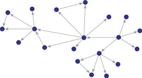
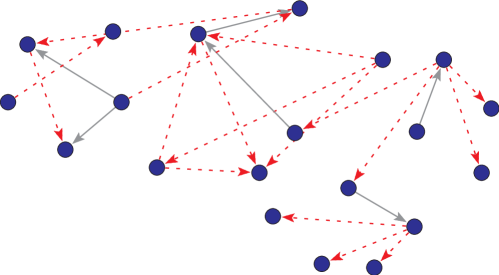
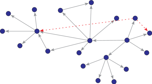
Edges in such networks of influence and diffusion have various interpretations. In virus or disease propagation, edges can be interpreted as who-infects-whom. In information propagation, edges are who-adopts-information-from-whom or who-listens-to-whom. In a viral marketing setting, edges can be understood as who-influences-whom.

The main premise of our work is that by observing many different contagions spreading among the nodes, we can infer the edges of the underlying propagation network. If node $v$ tends to get infected soon after node $u$ for many different contagions, then we can expect an edge $(u,v)$ to be present in the network. By exploring correlations in node infection times, we aim to recover the unobserved diffusion network.

Figure 2: The underlying true network over which contagions spread is illustrated on the top. Each subsequent layer depicts a cascade created by the diffusion of a particular contagion. For each cascade, nodes in gray are the “infected” nodes and the edges denote the direction in which the contagion propagated. Now, given only the node infection times in each cascade we aim to infer the connectivity of the underlying network $G^{*}$.

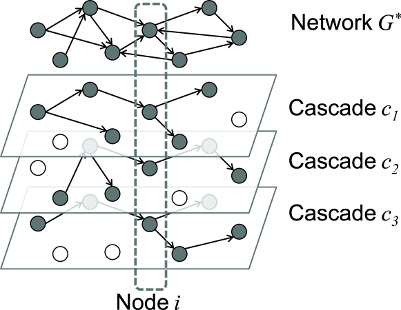
The concept of set of contagions over a network is illustrated in Figure 2. As a contagion spreads over the underlying network it creates a trace, called cascade. Nodes of the cascade are the nodes of the network that got infected by the contagion and edges of the cascade represent edges of the network over which the contagion actually spread. On the top of Figure 2, the underlying true network over which contagions spread is illustrated. Each subsequent layer depicts a cascade created by a particular contagion. A priori, we do not know the connectivity of the underlying true network and our aim is to infer this connectivity using the infection times of nodes in many cascades.

We develop NetInf, a scalable algorithm for inferring networks of diffusion and influence. We first formulate a generative probabilistic model of how, on a fixed hypothetical network, contagions spread as directed trees (i.e., a node infects many other nodes) through the network. Since we only observe times when nodes get infected, there are many possible ways of the contagion could have propagated through the network that are consistent with the observed data. In order to infer the network we have to consider all possible ways of the contagion spreading through the network. Thus, naive computation of the model takes exponential time since there is a combinatorially large number of propagation trees. We show that, perhaps surprisingly, computations over this super-exponential set of trees can be performed in polynomial (cubic) time. However, under such model, the network inference problem is still intractable. Thus, we introduce a tractable approximation, and show that the objective function can be both efficiently computed and efficiently optimized. By exploiting a diminishing returns property of the problem, we prove that NetInf infers near-optimal networks. We also speed-up NetInf by exploiting the local structure of the objective function and by using lazy evaluations [Leskovec et al. (2007)].

In a broader context, our work here is related to the network structure learning of probabilistic directed graphical models [Friedman et al. (1999), Getoor et al. (2003)] where heuristic greedy hill-climbing or stochastic search that both offer no performance guarantees are usually used in practice. In contrast, our work here provides a novel formulation and a tractable polynomial time algorithm for inferring directed networks together with an approximation guarantee that ensures the inferred networks will be of near-optimal quality.

Our results on synthetic datasets show that we can reliably infer an underlying propagation and influence network, regardless of the overall network structure. Validation on real and synthetic datasets shows that NetInf outperforms a baseline heuristic by an order of magnitude and correctly discovers more than 90% of the edges. We apply our algorithm to a real Web information propagation dataset of 170 million blog and news articles over a one year period. Our results show that online news propagation networks tend to have a core-periphery structure with a small set of core blog and news media websites that diffuse information to the rest of the Web, news media websites tend to diffuse the news faster than blogs and blogs keep discussing about news longer time than media websites.

Inferring how information or viruses propagate over networks is crucial for a better understanding of diffusion in networks. By modeling the structure of the propagation network, we can gain insight into positions and roles various nodes play in the diffusion process and assess the range of influence of nodes in the network.

The rest of the paper is organized as follows. Section 2 is devoted to the statement of the problem, the formulation of the model and the optimization problem. In section 3, an efficient reformulation of the optimization problem is proposed and its solution is presented. Experimental evaluation using synthetic and MemeTracker data are shown in section 4. We conclude with related work in section 5 and discussion of our results in section 6.

2 Diffusion network inference problem

We next formally describe the problem where contagions propagate over an unknown static directed network and create cascades. For each cascade we observe times when nodes got infected but not who infected them. The goal then is to infer the unknown network over which contagions originally propagated. In an information diffusion setting, each contagion corresponds to a different piece of information that spreads over the network and all we observe are the times when particular nodes adopted or mentioned particular information. The task then is to infer the network where a directed edge $(u,v)$ carries the semantics that node $v$ tends to get influenced by node $u$ (i.e., mentions or adopts the information after node $u$ does so as well).

2.1 Problem statement

Given a hidden directed network $G^{*}$, we observe multiple contagions spreading over it. As the contagion $c$ propagates over the network, it leaves a trace, a cascade, in the form of a set of triples $(u,v,t_{v})_{c}$, which means that contagion $c$ reached node $v$ at time $t_{v}$ by spreading from node $u$ (i.e., by propagating over the edge $(u,v)$). We denote the fact that the cascade initially starts from some active node $v$ at time $t_{v}$ as $(\emptyset,v,t_{v})_{c}$.

Now, we only get to observe the time $t_{v}$ when contagion $c$ reached node $v$ but not how it reached the node $v$, i.e., we only know that $v$ got infected by one of its neighbors in the network but do not know who $v$’s neighbors are and who of them infected $v$. Thus, instead of observing the triples $(u,v,t_{v})_{c}$ that fully specify the trace of the contagion $c$ through the network, we only get to observe pairs $(v,t_{v})_{c}$ that describe the time $t_{v}$ when node $v$ got infected by the contagion $c$. Now, given such data about node infection times for many different contagions, we aim to recover the unobserved directed network $G^{*}$, i.e., the network over which the contagions originally spread.

We use the term hit time $t_{u}$ to refer to the time when a cascade created by a contagion hits (infects, causes the adoption by) a particular node $u$. In practice, many contagions do not hit all the nodes of the network. Simply, if a contagion hits all the nodes this means it will infect every node of the network. In real-life most cascades created by contagions are relatively small. Thus, if a node $u$ is not hit by a cascade, then we set $t_{u}=\infty$. Then, the observed data about a cascade $c$ is specified by the vector $\mathbf{t_{c}}=[t_{1},\dots,t_{n}]$ of hit times, where $n$ is the number of nodes in $G^{*}$, and $t_{i}$ is the time when node $i$ got infected by the contagion $c$ ($t_{i}=\infty$ if $i$ did not get infected by $c$).

Our goal now is to infer the network $G^{*}$. In order to solve this problem we first define the probabilistic model of how contagions spread over the edges of the network. We first specify the contagion transmission model $P_{c}(u,v)$ that describes how likely is that node $u$ spreads the contagion $c$ to node $v$. Based on the model we then describe the probability $P(c|T)$ that the contagion $c$ propagated in a particular cascade tree pattern $T=(V_{T},E_{T})$, where tree $T$ simply specifies which nodes infected which other nodes (e.g., see Figure 2). Last, we define $P(c|G)$, which is the probability that cascade $c$ occurs in a network $G$. And then, under this model, we show how to estimate a (near-)maximum likelihood network $\hat{G}$, i.e., the network $\hat{G}$ that (approximately) maximizes the probability of cascades $c$ occurring in it.

2.2 Cascade Transmission Model

We start by formulating the probabilistic model of how contagions diffuse over the network. We build on the Independent Cascade Model [Kempe et al. (2003)] which posits that an infected node infects each of its neighbors in the network $G$ independently at random with some small chosen probability. This model implicitly assumes that every node $v$ in the cascade $c$ is infected by at most one node $u$. That is, it only matters when the first neighbor of $v$ infects it and all infections that come afterwards have no impact. Note that $v$ can have multiple of its neighbors infected but only one neighbor actually activates $v$. Thus, the structure of a cascade created by the diffusion of contagion $c$ is fully described by a directed tree $T$, that is contained in the directed graph $G$, i.e., since the contagion can only spread over the edges of $G$ and each node can only be infected by at most one other node, the pattern in which the contagion propagated is a tree and a subgraph of $G$. Refer to Figure 2 for an illustration of a network and a set of cascades created by contagions diffusing over it.

Probability of an individual transmission. The Independent Contagion Model only implicitly models time through the epochs of the propagation. We thus formulate a variant of the model that preserves the tree structure of cascades and also incorporates the notion of time.

We think of our model of how a contagion transmits from $u$ to $v$ in two steps. When a new node $u$ gets infected it gets a chance to transmit the contagion to each of its currently uninfected neighbors $w$ independently with some small probability $\beta$. If the contagion is transmitted we then sample the incubation time, i.e., how long after $w$ got infected, $w$ will get a chance to infect its (at that time uninfected) neighbors. Note that cascades in this model are necessarily trees since node $u$ only gets to infect neighbors $w$ that have not yet been infected.

First, we define the probability $P_{c}(u,v)$ that a node $u$ spreads the cascade to a node $v$, i.e., a node $u$ influences/infects/transmits contagion $c$ to a node $v$. Formally, $P_{c}(u,v)$ specifies the conditional probability of observing cascade $c$ spreading from $u$ to $v$.

Consider a pair of nodes $u$ and $v$, connected by a directed edge $(u,v)$ and the corresponding hit times $(u,t_{u})_{c}$ and $(v,t_{v})_{c}$. Since the contagion can only propagate forward in time, if node $u$ got infected after node $v$ ($t_{u}>t_{v}$) then $P_{c}(u,v)=0$, i.e., nodes can not influence nodes from the past. On the other hand (if $t_{u}<t_{v}$) we make no assumptions about the properties and shape of $P_{c}(u,v)$. To build some intuition, we can think that the probability of propagation $P_{c}(u,v)$ between a pair of nodes $u$ and $v$ is decreasing in the difference of their infection times, i.e., the farther apart in time the two nodes get infected the less likely they are to infect one another.

However, we note that our approach allows for the contagion transmission model $P_{c}(u,v)$ to be arbitrarily complicated as it can also depend on the properties of the contagion $c$ as well as the properties of the nodes and edges. For example, in a disease propagation scenario, node attributes could include information about the individual’s socio-economic status, commute patterns, disease history and so on, and the contagion properties would include the strength and the type of the virus. This allows for great flexibility in the cascade transmission models as the probability of infection depends on the parameters of the disease and properties of the nodes.

Symbol	Description
$G(V,E)$	Directed graph with nodes $V$ and edges $E$ over which contagions spread
$\beta$	Probability that contagion propagates over an edge of $G$
$\alpha$	Incubation time model parameter (refer to Eq. 1)
$E_{\varepsilon}$	Set of $\varepsilon$-edges, $E\cap E_{\varepsilon}=\emptyset$ and $E\cup E_{\varepsilon}=V\times V$
$c$	Contagion that spreads over $G$
$t_{u}$	Time when node $u$ got hit (infected) by a particular cascade
$\mathbf{t}_{c}$	Set of node hit times in cascade $c$. $\mathbf{t}_{c}[i]=\infty$ if node $i$ did not participate in $c$
$\Delta_{u,v}$	Time difference between the node hit times $t_{v}-t_{u}$ in a particular cascade
$C=\{(c,\mathbf{t}_{c})\}$	Set of contagions $c$ and corresponding hit times, i.e., the observed data
$\mathcal{T}_{c}(G)$	Set of all possible propagation trees of cascade $c$ on graph $G$
$T(V_{T},E_{T})$	Cascade propagation tree, $T\in\mathcal{T}_{c}(G)$
$V_{T}$	Node set of $T$, $V_{T}=\{i\ |\ i\in V\text{and}\ \mathbf{t}_{c}[i]<\infty\}$
$E_{T}$	Edge set of $T$, $E_{T}\subseteq E\cup E_{\varepsilon}$

Table 1: Table of symbols.

Purely for simplicity, in the rest of the paper we assume the simplest and most intuitive model where the probability of transmission depends only on the time difference between the node hit times $\Delta_{u,v}=t_{v}-t_{u}$. We consider two different models for the incubation time distribution $\Delta_{u,v}$, an exponential and a power-law model, each with parameter $\alpha$:

$$P_{c}(u,v)=P_{c}(\Delta_{u,v})\propto e^{-\frac{\Delta_{u,v}}{\alpha}}\mbox{ and }P_{c}(u,v)=P_{c}(\Delta_{u,v})\propto\frac{1}{\Delta_{u,v}^{\alpha}}.$$ (1)

Both the power-law and exponential waiting time models have been argued for in the literature [Barabási (2005), Leskovec et al. (2007), Malmgren et al. (2008)]. In the end, our algorithm does not depend on the particular choice of the incubation time distribution and more complicated non-monotonic and multimodal functions can easily be chosen [Crane and Sornette (2008), Wallinga and Teunis (2004), Gomez-Rodriguez et al. (2011)]. Also, we interpret $\infty+\Delta_{u,v}=\infty$, i.e., if $t_{u}=\infty$, then $t_{v}=\infty$ with probability $1$. Note that the parameter $\alpha$ can potentially be different for each edge in the network.

Considering the above model in a generative sense, we can think that the cascade $c$ reaches node $u$ at time $t_{u}$, and we now need to generate the time $t_{v}$ when $u$ spreads the cascade to node $v$. As cascades generally do not infect all the nodes of the network, we need to explicitly model the probability that the cascade stops. With probability $(1-\beta)$, the cascade stops, and never reaches $v$, thus $t_{v}=\infty$. With probability $\beta$, the cascade transmits over the edge $(u,v)$, and the hit time $t_{v}$ is set to $t_{u}+\Delta_{u,v}$, where $\Delta_{u,v}$ is the incubation time that passed between the hit times $t_{u}$ and $t_{v}$.

Likelihood of a cascade spreading in a given tree pattern $\bf T$. Next we calculate the likelihood $P(c|T)$ that contagion $c$ in a graph $G$ propagated in a particular tree pattern $T(V_{T},E_{T})$ under some assumptions. This means we want to assess the probability that a cascade $c$ with hit times $\mathbf{t}_{c}$ propagated in a particular tree pattern $T$.

Due to our modeling assumption that cascades are trees the likelihood is simply:

$$P(c|T)=\prod_{(u,v)\in E_{T}}\beta P_{c}(u,v)\prod_{u\in V_{T},(u,x)\in E\backslash E_{T}}(1-\beta),$$ (2)

where $E_{T}$ is the edge set and $V_{T}$ is the vertex set of tree $T$. Note that $V_{T}$ is the set of nodes that got infected by $c$, i.e., $V_{T}\subset V$ and contains elements $i$ of $\mathbf{t}_{c}$ where $\mathbf{t}_{c}(i)<\infty$. The above expression has an intuitive explanation. Since the cascade spread in tree pattern $T$, the contagion successfully propagated along those edges. And, along the edges where the contagion did not spread, the cascade had to stop. Here, we assume independence between edges to simplify the problem. Despite this simplification, we later show empirically that NetInf works well in practice

Moreover, $P(c|T)$ can be rewritten as:

$$P(c|T)=\beta^{q}(1-\beta)^{r}\prod_{(u,v)\in E_{T}}P_{c}(u,v),$$ (3)

where $q=|E_{T}|=|V_{T}|-1$ is the number of edges in $T$ and counts the edges over which the contagion successfully propagated. Similarly, $r$ counts the number of edges that did not activate and failed to transmit the contagion: $r=\sum_{u\in V_{T}}d_{out}(u)-q$, and $d_{out}(u)$ is the out-degree of node $u$ in graph $G$.

We conclude with an observation that will come very handy later. Examining Eq. 3 we notice that the first part of the equation before the product sign does not depend on the edge set $E_{T}$ but only on the vertex set $V_{T}$ of the tree $T$. This means that the first part is constant for all trees $T$ with the same vertex set $V_{T}$ but possibly different edge sets $E_{T}$. For example, this means that for a fixed $G$ and $c$ maximizing $P(c|T)$ with respect to $T$ (i.e., finding the most probable tree), does not depend on the second product of Eq. 2. This means that when optimizing, one only needs to focus on the first product where the edges of the tree $T$ simply specify how the cascade spreads, i.e., every node in the cascade gets influenced by exactly one node, that is, its parent.

Cascade likelihood. We just defined the likelihood $P(c|T)$ that a single contagion $c$ propagates in a particular tree pattern $T$. Now, our aim is to compute $P(c|G)$, the probability that a cascade $c$ occurs in a graph $G$. Note that we observe only the node infection times while the exact propagation tree $T$ (who-infected-whom) is unknown. In general, over a given graph $G$ there may be multiple different propagation trees $T$ that are consistent with the observed data. For example, Figure 3 shows three different cascade propagation paths (trees $T$) that are all consistent with the observed data $\mathbf{t}_{c}=(t_{a}=1,t_{c}=2,t_{b}=3,t_{e}=4)$

Figure 3: Different propagation trees $T$ of cascade $c$ that are all consistent with observed node hit times $c=(t_{a}=1,t_{c}=2,t_{b}=3,t_{e}=4)$. In each case, wider edges compose the tree, while thinner edges are the rest of the edges of the network $G$.

So, we need to combine the probabilities of individual propagation trees into a probability of a cascade $c$. We achieve this by considering all possible propagation trees $T$ that are supported by network $G$, i.e., all possible ways in which cascade $c$ could have spread over $G$:

$$P(c|G)=\sum_{T\in\mathcal{T}_{c}(G)}P(c|T)P(T|G),$$ (4)

where $c$ is a cascade and $\mathcal{T}_{c}(G)$ is the set of all the directed connected spanning trees on a subgraph of $G$ induced by the nodes that got hit by cascade $c$. Note that even though the sum ranges over all possible spanning trees $T\in\mathcal{T}_{c}(G)$, in case $T$ is inconsistent with the observed data, then $P(c|T)=0$.

Assuming that all trees are a priori equally likely (i.e., $P(T|G)=1/|\mathcal{T}_{c}(G)|$) and using the observation from Equation 3 we obtain:

$$P(c|G)\propto\sum_{T\in\mathcal{T}_{c}(G)}\prod_{(u,v)\in E_{T}}P_{c}(u,v).$$ (5)

Basically, the graph $G$ defines the skeleton over which the cascades can propagate and $T$ defines a particular possible propagation tree. There may be many possible trees that explain a single cascade (see Fig. 3), and since we do not know in which particular tree pattern the cascade really propagated, we need to consider all possible propagation trees $T$ in $\mathcal{T}_{c}(G)$. Thus, the sum over $T$ is a sum over all directed spanning trees of the graph induced by the vertices that got hit by the cascade $c$.

We just computed the probability of a single cascade $c$ occurring in $G$, and we now define the probability of a set of cascades $C$ occurring in $G$ simply as:

$$P(C|G)=\prod_{c\in C}P(c|G),$$ (6)

where we again assume conditional independence between cascades given the graph $G$.

2.3 Estimating the network that maximizes the cascade likelihood

Now that once we have formulated the cascade transmission model, we now state the diffusion network inference problem, where the goal is to find $\hat{G}$ that solves the following optimization problem:

Problem 1

Given a set of node infection times $\mathbf{t}_{c}$ for a set of cascades $c\in C$, a propagation probability parameter $\beta$ and an incubation time distribution $P_{c}(u,v)$, find the network $\hat{G}$ such that:

$$\hat{G}=\operatorname*{argmax}_{|G|\leq k}P(C|G),$$ (7)

where the maximization is over all directed graphs $G$ of at most $k$ edges, and $P(C|G)$ is defined by equations 6, 4 and 2.

We include the constraint on the number of edges in $\hat{G}$ simply because we seek for a sparse solution, since real graphs are sparse. We discuss how to choose $k$ in further sections of the paper.

The above optimization problem seems wildly intractable. To evaluate Eq. (6), we need to compute Eq. (4) for each cascade $c$, i.e., the sum over all possible spanning trees $T$. The number of trees can be super-exponential in the size of $G$ but perhaps surprisingly, this super-exponential sum can be performed in time polynomial in the number $n$ of nodes in the graph $G$, by applying Kirchhoff’s matrix tree theorem [Knuth (1968)]:

Theorem 1 ([Tutte (1948)])

If we construct a matrix $A$ such that $a_{i,j}=\sum_{k}w_{k,j}$ if $i=j$ and $a_{i,j}=-w_{i,j}$ if $i\neq j$ and if $A_{x,y}$ is the matrix created by removing any row $x$ and column $y$ from $A$, then

$$(-1)^{x+y}\det(A_{x,y})=\sum_{T\in A}\prod_{(i,j)\in T}w_{i,j},$$ (8)

where $T$ is each directed spanning tree in $A$.

In our case, we set $w_{i,j}$ to be simply $P_{c}(i,j)$ and we compute the product of the determinants of $|C|$ matrices, one for each cascade, which is exactly Eq. 4. Note that since edges $(i,j)$ where $t_{i}\geq t_{j}$ have weight 0 (i.e., they are not present), given a fixed cascade $c$, the collection of edges with positive weight forms a directed acyclic graph (DAG). A DAG with a time-ordered labeling of its nodes has an upper triangular connectivity matrix. Thus, the matrix $A_{x,y}$ of Theorem 1 is, by construction, upper triangular. Fortunately, the determinant of an upper triangular matrix is simply the product of the elements of its diagonal. This means that instead of using super-exponential time, we are now able to evaluate Eq. 6 in time $(|C|\cdot|V|^{2})$ (the time required to build $A_{x,y}$ and compute the determinant for each of the $|C|$ cascades).

However, this does not completely solve our problem for two reasons: First, while cuadratic time is a drastic improvement over a super-exponential computation, it is still too expensive for the large graphs that we want to consider. Second, we can use the above result only to evaluate the quality of a particular graph $G$, while our goal is to find the best graph $\hat{G}$. To do this, we would need to search over all graphs $G$ to find the best one. Again, as there is a super-exponential number of graphs, this is not practical. To circumvent this one could propose some ad hoc search heuristics, like hill-climbing. However, due to the combinatorial nature of the likelihood function, such a procedure would likely be prone to local maxima. We leave the question of efficient maximization of Eq. 4 where $P(c|G)$ considers all possible propagation trees as an interesting open problem.

3 Alternative formulation and the NetInf algorithm

The diffusion network inference problem defined in the previous section does not seem to allow for an efficient solution. We now propose an alternative formulation of the problem that is tractable both to compute and also to optimize.

3.1 An alternative formulation

We use the same tree cascade formation model as in the previous section. However, we compute an approximation of the likelihood of a single cascade by considering only the most likely tree instead of all possible propagation trees. We show that this approximate likelihood is tractable to compute. Moreover, we also devise an algorithm that provably finds networks with near optimal approximate likelihood. In the remainder of this section, we informally write likelihood and log-likelihood even though they are approximations. However, all approximations are clearly indicated.

First we introduce the concept of $\varepsilon$-edges to account for the fact that nodes may get infected for reasons other than the network influence. For example, in online media, not all the information propagates via the network, as some is also pushed onto the network by the mass media [Katz and Lazarsfeld (1955), Watts and Dodds (2007)] and thus a disconnected cascade can be created. Similarly, in viral marketing, a person may purchase a product due to the influence of peers (i.e., network effect) or for some other reason (e.g., seing a commercial on TV) [Leskovec et al. (2006)].

Modeling external influence via $\varepsilon$-edges. To account for such phenomena when a cascade “jumps” across the network we can think of creating an additional node $x$ that represents an external influence and can infect any other node $u$ with small probability. We then connect the external influence node $x$ to every other node $u$ with an $\varepsilon$-edge. And then every node $u$ can get infected by the external source $x$ with a very small probability $\varepsilon$. For example, in case of information diffusion in the blogosphere, such a node $x$ could model the effect of blogs getting infected by the mainstream media.

However, if we were to adopt this approach and insert an additional external influence node $x$ into our data, we would also need to infer the edges pointing out of $x$, which would make our problem even harder. Thus, in order to capture the effect of external influence, we introduce a concept of $\varepsilon$-edge. If there is not a network edge between a node $i$ and a node $j$ in the network, we add an $\varepsilon$-edge and then node $i$ can infect node $j$ with a small probability $\varepsilon$. Even though adding $\varepsilon$-edges makes our graph $G$ a clique (i.e., the union of network edges and $\varepsilon$-edges creates a clique), the $\varepsilon$-edges play the role of external influence node.

Thus, we now think of graph $G$ as a fully connected graph of two disjoint sets of edges, the network edge set $E$ and the $\varepsilon$-edge set $E_{\varepsilon}$, i.e., $E\cap E_{\varepsilon}=\emptyset$ and $E\cup E_{\varepsilon}=V\times V$.

Now, any cascade propagation tree $T$ is a combination of network and $\varepsilon$-edges. As we model the external influence via the $\varepsilon$-edges, the probability of a cascade $c$ occurring in tree $T$ (i.e., the analog of Eq. 2) can now be computed as:

$$P(c|T)=\prod_{u\in V_{T}}\ \ \prod_{v\in V}P_{c}^{\prime}(u,v),$$ (9)

where we compute the transmission probability $P_{c}^{\prime}(u,v)$ as follows:

$$P_{c}^{\prime}(u,v)=\begin{cases}\beta P_{c}(t_{v}-t_{u})&\text{if $t_{u}<t_{v}$ and $(u,v)\in E_{T}\cap E$ \ \ \ \ \ \ \ {\em$(u,v)$ is network edge}}\\ \varepsilon P_{c}(t_{v}-t_{u})&\text{if $t_{u}<t_{v}$ and $(u,v)\in E_{T}\cap E_{\varepsilon}$ \ \ \ \ \ {\em$(u,v)$ is $\varepsilon$-edge}}\\ 1-\beta&\text{if $t_{v}=\infty$ and $(u,v)\in E\backslash E_{T}$ \ \ \ \ \ \ \ \ \ {\em$v$ is not infected, network edge}}\\ 1-\varepsilon&\text{if $t_{v}=\infty$ and $(u,v)\in E_{\varepsilon}\backslash E_{T}$ \ \ \ \ \ \ \ {\em$v$ is not infected, $\varepsilon$-edge}}\\ 0&\text{else (\emph{i.e.}, $t_{u}\geq t_{v}$).}\\ \end{cases}$$

Note that above we distinguish four type of edges: network and $\varepsilon$-edges that participated in the diffusion of the contagion and network and $\varepsilon$-edges that did not participate in the diffusion.

Figure 4 further illustrates this concept. First, Figure 4(a) shows an example of a graph $G$ on five nodes and four network edges $E$ (solid lines), and any other possible edge is the $\varepsilon$-edge (dashed lines). Then, Figure 4(b) shows an example of a propagation tree $T=\{(a,b),(b,c),(b,d)\}$ in graph $G$. We only show the edges that play a role in Eq. 9 and label them with four different types: (a) network edges that transmitted the contagion, (b) $\varepsilon$-edges that transmitted the contagion, (c) network edges that failed to transmit the contagion, and (d) $\varepsilon$-edges that failed to transmit the contagion.

(a) Graph $G$ on five vertices and four network edges (solid edges). $\varepsilon$-edges shown as dashed lines.

(b) Cascade propagation tree $T=\{(a,b),(b,c),(b,d)\}$

Figure 4: (a) Graph $G$: Network edges $E$ are shown as solid, and $\varepsilon$-edges are shown as dashed lines. (b) Propagation tree $T=\{(a,b),(b,c),(b,d)\}$. Four types of edges are labeled: (i) network edges that transmitted the contagion (solid bold), (ii) $\varepsilon$-edges that transmitted the contagion (dashed bold), (iii) network edges that failed to transmit the contagion (solid), and (iv) $\varepsilon$-edges that failed to transmit the contagion (dashed).

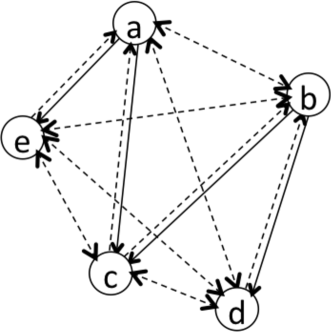
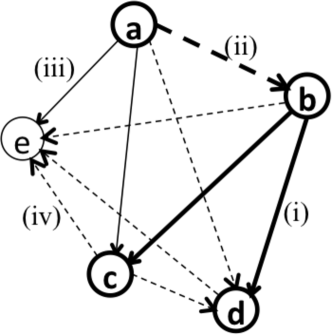
We can now rewrite the cascade likelihood $P(c|T)$ as combination of products of edge-types and the product over the edge incubation times:

$$P(c|T) = \beta^{q}\ \varepsilon^{q^{\prime}}\ (1-\beta)^{s}\ (1-\varepsilon)^{s^{\prime}}\prod_{(u,v)\in E_{T}}P_{c}(v,u)$$ (10)

$$\approx \beta^{q}\ \varepsilon^{q^{\prime}}\ (1-\varepsilon)^{s+s^{\prime}}\prod_{(u,v)\in E_{T}}P_{c}(v,u),$$ (11)

where $q$ is the number of network edges in $T$ (type (a) edges in Fig. 4(b)), $q^{\prime}$ is the number of $\varepsilon$-edges in $T$, $s$ is the number of network edges that did not transmit and $s^{\prime}$ is the number of $\varepsilon$-edges that did not transmit. Note that the above approximation is valid since real networks are sparse and cascades are generally small, and hence $s^{\prime}\gg s$. Thus, even though $\beta\gg\varepsilon$ we expect $(1-\beta)^{s}$ to be of about same order of magnitude as $(1-\varepsilon)^{s^{\prime}}$.

The formulation in Equation 11 has several benefits. Due to the introduction of $\varepsilon$-edges the likelihood $P(c|T)$ is always positive. For example, even if we consider graph $G$ with no edges, $P(c|T)$ is still well defined as we can explain the tree $T$ via the diffusion over the $\varepsilon$-edges. A second benefit that will become very useful later is that the likelihood now becomes monotonic in the network edges of $G$. This means that adding an edge to $G$ (i.e., converting $\varepsilon$-edge into a network edge) only increases the likelihood.

Considering only the most likely propagation tree. So far we introduced the concept of $\varepsilon$-edges to model the external influence or diffusion that is exogenous to the network, and introduce an approximation to treat all edges that did not participate in the diffusion as $\varepsilon$-edges.

Now we consider the last approximation, where instead of considering all possible cascade propagation trees $T$, we only consider the most likely cascade propagation trees $T$:

$$P(C|G)=\prod_{c\in C}\ \sum_{T\in\mathcal{T}_{c}(G)}P(c|T)\approx\prod_{c\in C}\ \max_{T\in\mathcal{T}_{c}(G)}P(c|T).$$ (12)

Thus now we aim to solve the network inference problem by finding a graph $G$ that maximizes Equation 12, where $P(c|T)$ is defined in Equation 11.

This formulation simplifies the original network inference problem by considering the most likely (best) propagation tree $T$ per cascade $c$ instead of considering all possible propagation trees $T$ for each cascade $c$. Although in some cases we expect the likelihood of $c$ with respect to the true tree $T^{\prime}$ to be much higher than that with respect to any competing tree $T^{\prime\prime}$ and thus the probability mass will be concentrated at $T^{\prime}$, there might be some cases in which the probability mass does not concentrate on one particular T. However, we run extensive experiments on small networks with different structures in which both the original network inference problem and the alternative formulation can be solved using exhaustive search. Our experimental results looked really similar and the results were indistinguishable. Therefore, we consider our approximation to work well in practice.

For convenience, we work with the log-likelihood $\log P(c|T)$ rather than likelihood $P(c|T)$. Moreover, instead of directly maximizing the log-likelihood we equivalently maximize the following objective function that defines the improvement of log-likelihood for cascade $c$ occurring in graph $G$ over $c$ occurring in an empty graph $\bar{K}$ (i.e., graph with only $\varepsilon$-edges and no network edges):

$$F_{c}(G)=\max_{T\in\mathcal{T}_{c}(G)}\log P(c|T)-\max_{T\in\mathcal{T}_{c}(\bar{K})}\log P(c|T).$$ (13)

Maximizing Equation (12) is equivalent to maximizing the following log-likelihood function:

$$F_{C}(G)=\sum_{c\in C}F_{c}(G).$$ (14)

We now expand Eq. (13) and obtain an instance of a simplified diffusion network inference problem:

$$\hat{G}=\arg\max_{G}F_{C}(G)=\sum_{c\in C}\max_{T\in\mathcal{T}_{c}(G)}\sum_{(i,j)\in E_{T}}w_{c}(i,j),$$ (15)

where $w_{c}(i,j)=\log P_{c}^{\prime}(i,j)-\log\varepsilon$ is a non-negative weight which can be interpreted as the improvement in log-likelihood of edge $(i,j)$ under the most likely propagation tree $T$ in $G$. Note that by the approximation in Equation 11 one can ignore the contribution of edges that did not participate in a particular cascade $c$. The contribution of these edges is constant, i.e., independent of the particular shape that propagation tree $T$ takes. This is due to the fact that each spanning tree $T$ of $G$ with node set $V_{T}$ has $|V_{T}|-1$ (network and $\varepsilon$-) edges that participated in the cascade, and all remaining edges stopped the cascade from spreading. The number of non-spreading edges depends only on the node set $V_{T}$ but not the edge set $E_{T}$. Thus, the tree $T$ that maximizes $P(c|T)$ also maximizes $\sum_{(i,j)\in E_{T}}w_{c}(i,j)$.

Since $T$ is a tree that maximizes the sum of the edge weights this means that the most likely propagation tree $T$ is simply the maximum weight directed spanning tree of nodes $V_{T}$, where each edge $(i,j)$ has weight $w_{c}(i,j)$, and $F_{c}(G)$ is simply the sum of the weights of edges in $T$.

We also observe that since edges $(i,j)$ where $t_{i}\geq t_{j}$ have weight 0 (i.e., such edges are not present) then the outgoing edges of any node $u$ only point forward in time, i.e., a node can not infect already infected nodes. Thus for a fixed cascade $c$, the collection of edges with positive weight forms a directed acyclic graph (DAG).

Now we use the fact that the collection of edges with positive weights forms a directed acyclic graph by observing that the maximum weight directed spanning tree of a DAG can be computed efficiently:

Proposition 1

In a DAG $D(V,E,w)$ with vertex set $V$ and nonnegative edge weights $w$, the maximum weight directed spanning tree can be found by choosing, for each node $v$, an incoming edge $(u,v)$ with maximum weight $w(u,v)$.

Proof 3.2.

The score

$$S(T)=\sum_{(i,j)\in T}w(i,j)=\sum_{i\in V}w(Par_{T}(i),i)$$

of a tree $T$ is the sum of the incoming edge weights $w(Par_{T}(i),i)$ for each node $i$, where $Par_{T}(i)$ is the parent of node $i$ in $T$ (and the root is handled appropriately). Now,

$$\max_{T}S(T)=\max_{T}\sum_{(i,j)\in T}w(i,j)=\sum_{i\in V}\max_{Par_{T}(i)}w(Par_{T}(i),i).$$

Latter equality follows from the fact that since $G$ is a DAG, the maximization can be done independently for each node without creating any cycles.

This proposition is a special case of the more general maximum spanning tree (MST) problem in directed graphs [Edmonds (1967)]. The important fact now is that we can find the best propagation tree $T$ in time $O(|V_{T}|D_{in})$, i.e., linear in the number of edges and the maximum in-degree $D_{in}=\max_{u\in V_{T}}d_{in}(u)$ by simply selecting an incoming edge of highest weight for each node $u\in V_{T}$. Algorithm 1 provides the pseudocode to efficiently compute the maximum weight directed spanning tree of a DAG.

Algorithm 1 Maximum weight directed spanning tree of a DAG

0:  Weighted directed acyclic graph $D(V,E,w)$

  $T\leftarrow\{\}$

  for all $i\in V$ do

     $Par_{T}(i)=\arg\max_{j}w(j,i)$

     $T\leftarrow T\cup\{(Par_{T}(i),j)\}$

  return  $T$

Putting it all together we have shown how to efficiently evaluate the log-likelihood $F_{C}(G)$ of a graph $G$. To find the most likely tree $T$ for a single cascade takes $O(|V_{T}|D_{in})$, and this has to be done for a total of $|C|$ cascades. Interestingly, this is independent of the size of graph $G$ and only depends on the amount of observed data (i.e., size and the number of cascades).

3.2 The NetInf algorithm for efficient maximization of $\bf F_{C}(G)$

Now we aim to find graph $G$ that maximizes the log-likelihood $F_{C}(G)$. First we notice that by construction $F_{C}(\bar{K})=0$, i.e., the empty graph has score 0. Moreover, we observe that the objective function $F_{C}$ is non-negative and monotonic. This means that $F_{C}(G)\leq F_{C}(G^{\prime})$ for graphs $G(V,E)$ and $G^{\prime}(V,E^{\prime})$, where $E\subseteq E^{\prime}$. Hence adding more edges to $G$ does not decrease the solution quality, and thus the complete graph maximizes $F_{C}$. Monotonicity can be shown by observing that, as edges are added to $G$, $\varepsilon$-edges are converted to network edges, and therefore the weight of any tree (and therefore the value of the maximum spanning tree) can only increase. However, since real-world social and information networks are usually sparse, we are interested in inferring a sparse graph $G$, that only contains some small number $k$ of edges. Thus we aim to solve:

Problem 3.3.

Given the infection times of a set of cascades $C$, probability of propagation $\beta$ and the incubation time distribution $P_{c}(i,j)$, find $\hat{G}$ that maximizes:

$$G^{*}=\operatorname*{argmax}_{|G|\leq k}F_{C}(G),$$ (16)

where the maximization is over all graphs $G$ of at most $k$ edges, and $F_{C}(G)$ is defined by Eqs. 14 and 15.

Naively searching over all $k$ edge graphs would take time exponential in $k$, which is intractable. Moreover, finding the optimal solution to Eq. (16) is NP-hard, so we cannot expect to find the optimal solution:

Theorem 3.4.

The network inference problem defined by equation (16) is NP-hard.

Proof 3.5.

By reduction from the MAX-$k$-COVER problem [Khuller et al. (1999)]. In MAX-$k$-COVER, we are given a finite set $W$, $|W|=n$ and a collection of subsets $S_{1},\dots,S_{m}\subseteq W$. The function

$$F_{MC}(A)=|\cup_{i\in A}S_{i}|$$

counts the number of elements of $W$ covered by sets indexed by $A$. Our goal is to pick a collection of $k$ subsets $A$ maximizing $F_{MC}$. We will produce a collection of $n$ cascades $C$ over a graph $G$ such that $\max_{|G|\leq k}F_{C}(G)=\max_{|A|\leq k}F_{MC}(A)$. Graph $G$ will be defined over the set of vertices $V=\{1,\dots,m\}\cup\{r\}$, i.e., there is one vertex for each set $S_{i}$ and one extra vertex $r$. For each element $s\in W$ we define a cascade which has time stamp $0$ associated with all nodes $i\in V$ such that $s\in S_{i}$, time stamp $1$ for node $r$ and $\infty$ for all remaining nodes.

Furthermore, we can choose the transmission model such that $w_{c}(i,r)=1$ whenever $s\in S_{i}$ and $w_{c}(i^{\prime},j^{\prime})=0$ for all remaining edges $(i^{\prime},j^{\prime})$, by choosing the parameters $\varepsilon$, $\alpha$ and $\beta$ appropriately. Since a directed spanning tree over a graph $G$ can contain at most one edge incoming to node $r$, its weight will be $1$ if $G$ contains any edge from a node $i$ to $r$ where $s\in S_{i}$, and $0$ otherwise. Thus, a graph $G$ of at most $k$ edges corresponds to a feasible solution $A_{G}$ to MAX-$k$-COVER where we pick sets $S_{i}$ whenever edge $(i,r)\in G$, and each solution $A$ to MAX-$k$-COVER corresponds to a feasible solution $G_{A}$ of (16). Furthermore, by construction, $F_{MC}(A_{G})=F_{C}(G)$. Thus, if we had an efficient algorithm for deciding whether there exists a graph $G$, $|G|\leq k$ such that $F_{C}(G)>c$, we could use the algorithm to decide whether there exists a solution $A$ to MAX-$k$-COVER with value at least $c$.

While finding the optimal solution is hard, we now show that $F_{C}$ satisfies submodularity, a natural diminishing returns property. The submodularity property allows us to efficiently find a provably near-optimal solution to this otherwise NP-hard optimization problem.

A set function $F:2^{W}\rightarrow\mathbb{R}$ that maps subsets of a finite set $W$ to the real numbers is submodular if for $A\subseteq B\subseteq W$ and $s\in W\setminus B$, it holds that

$$F(A\cup\{s\})-F(A)\geq F(B\cup\{s\})-F(B).$$

This simply says adding $s$ to the set $A$ increases the score more than adding $s$ to set $B$ ($A\subseteq B$).

Now we are ready to show the following result that enables us to find a near optimal network $G$:

Theorem 3.6.

Let $V$ be a set of nodes, and $C$ be a collection of cascades hitting the nodes $V$. Then $F_{C}(G)$ is a submodular function $F_{C}:2^{W}\rightarrow\mathbb{R}$ defined over subsets $W\subseteq V\times V$ of directed edges.

Proof 3.7.

Fix a cascade $c$, graphs $G\subseteq G^{\prime}$ and an edge $e=(r,s)$ not contained in $G^{\prime}$. We will show that $F_{c}(G\cup\{e\})-F_{c}(G)\geq F_{c}(G^{\prime}\cup\{e\})-F_{c}(G^{\prime})$. Since nonnegative linear combinations of submodular functions are submodular, the function $F_{C}(G)=\sum_{c\in C}F_{c}(G)$ is submodular as well. Let $w_{i,j}$ be the weight of edge $(i,j)$ in $G\cup\{e\}$, and $w^{\prime}_{i,j}$ be the weight in $G^{\prime}\cup\{e\}$. As argued before, the maximum weight directed spanning tree for DAGs is obtained by assigning to each node the incoming edge with maximum weight. Let $(i,s)$ be the edge incoming at $s$ of maximum weight in $G$, and $(i^{\prime},s)$ the maximum weight incoming edge in $G^{\prime}$. Since $G\subseteq G^{\prime}$ it holds that $w_{i,s}\leq w^{\prime}_{i^{\prime},s}$. Furthermore, $w_{r,s}=w^{\prime}_{r,s}$. Hence,

$$F_{c}(G\cup\{(r,s)\})-F_{c}(G) =\max(w_{i,s},w_{r,s})-w_{i,s}$$

$$\geq\max(w^{\prime}_{i^{\prime},s},w^{\prime}_{r,s})-w^{\prime}_{i^{\prime},s}$$

$$=F_{c}(G^{\prime}\cup\{(r,s)\})-F_{c}(G^{\prime}),$$

proving submodularity of $F_{c}$.

Maximizing submodular functions in general is NP-hard [Khuller et al. (1999)]. A commonly used heuristic is the greedy algorithm, which starts with an empty graph $\bar{K}$, and iteratively, in step $i$, adds the edge $e_{i}$ which maximizes the marginal gain:

$$e_{i}=\operatorname*{argmax}_{e\in G\backslash G_{i-1}}F_{C}(G_{i-1}\cup\{e\})-F_{C}(G_{i-1}).$$ (17)

The algorithm stops once it has selected $k$ edges, and returns the solution $\hat{G}=\{e_{1},\dots,e_{k}\}$. The stopping criteria, i.e., value of $k$, can be based on some threshold of the marginal gain, of the number of estimated edges or another more sophisticated heuristic.

In our context we can think about the greedy algorithm as starting on an empty graph $\bar{K}$ with no network edges. In each iteration $i$, the algorithm adds to $G$ the edge $e_{i}$ that currently improves the most the value of the log-likelihood. Another way to view the greedy algorithm is that it starts on a fully connected graph $\bar{K}$ where all the edges are $\varepsilon$-edges. Then adding an edge to graph $G$ corresponds to that edge changing the type from $\varepsilon$-edge to a network edge. Thus our algorithm iteratively swaps $\varepsilon$-edges to network edges until $k$ network edges have been swapped (i.e., inserted into the network $G$).

Guarantees on the solution quality. Considering the NP-hardness of the problem, we might expect the greedy algorithm to perform arbitrarily bad. However, we will see that this is not the case. A fundamental result of Nemhauser et al. [Nemhauser et al. (1978)] proves that for monotonic submodular functions, the set $\hat{G}$ returned by the greedy algorithm obtains at least a constant fraction of $(1-1/e)\approx 63\%$ of the optimal value achievable using $k$ edges.

Moreover, we can acquire a tight online data-dependent bound on the solution quality:

Theorem 3.8 ([Leskovec et al. (2007)]).

For a graph $\hat{G}$, and each edge $e\notin\hat{G}$, let $\delta_{e}=F_{C}(\hat{G}\cup\{e\})-F_{C}(\hat{G})$. Let $e_{1},\ldots e_{B}$ be the sequence with $\delta_{e}$ in decreasing order, where $B$ is the total number of edges with marginal gain greater than $0$. Then,

$$\max_{|G|\leq k}F_{c}(G)\leq F_{c}(\hat{G})+\sum_{i=1}^{k}\delta_{e_{i}}.$$

Theorem 3.8 computes how far a given $\hat{G}$ (obtained by any algorithm) is from the unknown NP-hard to find optimum.

Speeding-up the NetInf algorithm. To make the algorithm scale to networks with thousands of nodes we speed-up the algorithm by several orders of magnitude by considering two following two improvements:

Localized update: Let $C_{i}$ be the subset of cascades that go through the node $i$ (i.e., cascades in which node $i$ is infected). Then consider that in some step $n$ the greedy algorithm selects the network edge $(j,i)$ with marginal gain $\delta_{j,i}$, and now we have to update the optimal tree of each cascade. We make a simple observation that adding the network edge $(j,i)$ may only change the optimal trees of the cascades in the set $C_{i}$ and thus we only need to revisit (and potentially update) the trees of cascades in $C_{i}$. Since cascades are local (i.e., each cascade hits only a relatively small subset of the network), this localized updating procedure speeds up the algorithm considerably.

Lazy evaluation: It can be used to drastically reduce the number of evaluations of marginal gains $F_{C}(G\cup\{e\})-F_{C}(G)$ [Leskovec et al. (2007)]. This procedure relies on the submodularity of $F_{C}$. The key idea behind lazy evaluations is the following. Suppose $G_{1},\dots,G_{k}$ is the sequence of graphs produced during iterations of the greedy algorithm. Now let us consider the marginal gain

$$\Delta_{e}(G_{i})=F_{C}(G_{i}\cup\{e\})-F_{C}(G_{i})$$

of adding some edge $e$ to any of these graphs. Due to the submodularity of $F_{C}$ it holds that $\Delta_{e}(G_{i})\geq\Delta_{e}(G_{j})$ whenever $i\leq j$. Thus, the marginal gains of $e$ can only monotonically decrease over the course of the greedy algorithm. This means that elements which achieve very little marginal gain at iteration $i$ cannot suddenly produce large marginal gain at subsequent iterations. This insight can be exploited by maintaining a priority queue data structure over the edges and their respective marginal gains. At each iteration, the greedy algorithm retrieves the highest weight (priority) edge. Since its value may have decreased from previous iterations, it recomputes its marginal benefit. If the marginal gain remains the same after recomputation, it has to be the edge with highest marginal gain, and the greedy algorithm will pick it. If it decreases, one reinserts the edge with its new weight into the priority queue and continues. Formal details and pseudo-code can be found in [Leskovec et al. (2007)].

As we will show later, these two improvements decrease the run time by several orders of magnitude with no loss in the solution quality. We call the algorithm that implements the greedy algorithm on this alternative formulation with the above speedups the NetInf algorithm (Algorithm 2). In addition, NetInf nicely lends itself to parallelization as likelihoods of individual cascades and likelihood improvements of individual new edges can simply be computed independently. This allows us to to tackle even bigger networks in shorter amounts of time.

A space and runtime complexity analysis of NetInf depends heavily of the structure of the network, and therefore it is necessary to make strong assumptions on the structure. Due to this, it is out of the scope of the paper to include a formal complexity analysis. Instead, we include an empirical runtime analysis in the following section.

Algorithm 2 The NetInf Algorithm

0:  Cascades and hit times $C=\{(c,\mathbf{t}_{c})\}$, number of edges $k$

  $G\leftarrow\bar{K}$

  for all $c\in C$ do

     $T_{c}\leftarrow dag\_tree(c)$ {Find most likely tree (Algorithm 1)}

  while $|G|<k$ do

     for all $(j,i)\notin G$ do

        $\delta_{j,i}=0$ {Marginal improvement of adding edge $(j,i)$ to G}

        $M_{j,i}\leftarrow\emptyset$

        for all $c:t_{j}<t_{i}$ in $c$ do

           Let $w_{c}(m,n)$ be the weight of $(m,n)$ in $G\cup\{(j,i)\}$

           if $w_{c}(j,i)\geq w_{c}(Par_{T_{c}}(i),i)$ then

              $\delta_{j,i}=\delta_{j,i}+w_{c}(j,i)-w_{c}(Par_{T_{c}}(i),i)$

              $M_{j,i}\leftarrow M_{j,i}\cup\{c\}$

     $(j^{*},i^{*})\leftarrow\arg\max_{(j,i)\in C\backslash G}\delta_{j,i}$

     $G\leftarrow G\cup\{(j^{*},i^{*})\}$

     for all $c\in M_{j^{*},i^{*}}$ do

        $Par_{T_{c}}(i^{*})\leftarrow j^{*}$

  return  G;

4 Experimental evaluation

In this section we proceed with the experimental evaluation of our proposed NetInf algorithm for inferring network of diffusion. We analyze the performance of NetInf on synthetic and real networks. We show that our algorithm performs surprisingly well, outperforms a heuristic baseline and correctly discovers more than 90% of the edges of a typical diffusion network.

4.1 Experiments on synthetic data

The goal of the experiments on synthetic data is to understand how the underlying network structure and the propagation model (exponential and power-law) affect the performance of our algorithm. The second goal is to evaluate the effect of simplification we had to make in order to arrive to an efficient network inference algorithm. Namely, we assume the contagion propagates in a tree pattern $T$ (i.e., exactly $E_{T}$ edges caused the propagation), consider only the most likely tree $T$ (Eq. 12), and treat non-propagating network edges as $\varepsilon$-edges (Eq. 11).

(a) FF: Cascades per edge

(b) FF: Cascade size

Figure 5: Number of cascades per edge and cascade sizes for a Forest Fire network ($1,024$ nodes, $1,477$ edges) with forward burning probability $0.20$, backward burning probability $0.17$ and exponential incubation time model with parameter $\alpha=1$ and propagation probability $\beta=0.5$. The cascade size distribution follows a power-law. We found the power-law coefficient using maximum likelihood estimation (MLE).

In general, in all our experiments we proceed as follows: We are given a true diffusion network $G^{*}$, and then we simulate the propagation of a set of contagions $c$ over the network $G^{*}$. Diffusion of each contagion creates a cascade and for each cascade, we record the node hit times $t_{u}$. Then, given these node hit times, we aim to recover the network $G^{*}$ using the NetInf algorithm. For example, Figure 1(a) shows a graph $G^{*}$ of 20 nodes and 23 directed edges. Using the exponential incubation time model and $\beta=0.2$ we generated $24$ cascades. Now given the node infection times, we aim to recover $G^{*}$. A baseline method (b) (described below) performed poorly while NetInf (c) recovered $G^{*}$ almost perfectly by making only two errors (red edges).

Experimental setup. Our experimental methodology is composed of the following steps:

1. Ground truth graph $G^{*}$

2. Cascade generation: Probability of propagation $\beta$, and the incubation time model with parameter $\alpha$.

3. Number of cascades

(1) Ground truth graph $G^{*}$: We consider two models of directed real-world networks to generate $G^{*}$, namely, the Forest Fire model [Leskovec et al. (2005)] and the Kronecker Graphs model [Leskovec and Faloutsos (2007)]. For Kronecker graphs, we consider three sets of parameters that produce networks with a very different global network structure: a random graph [Erdős and Rényi (1960)] (Kronecker parameter matrix $[0.5,0.5;0.5,0.5]$), a core-periphery network [Leskovec et al. (2008)] ($[0.962,0.535;0.535,0.107]$) and a network with hierarchical community structure [Clauset et al. (2008)] ($[0.962,0.107;0.107,0.962]$). The Forest Fire generates networks with power-law degree distributions that follow the densification power law [Barabási and Albert (1999), Leskovec et al. (2007)].

(2) Cascade propagation: We then simulate cascades on $G^{*}$ using the generative model defined in Section 2.1. For the simulation we need to choose the incubation time model (i.e., power-law or exponential and parameter $\alpha$). We also need to fix the parameter $\beta$, that controls probability of a cascade propagating over an edge. Intuitively, $\alpha$ controls how fast the cascade spreads (i.e., how long the incubation times are), while $\beta$ controls the size of the cascades. Large $\beta$ means cascades will likely be large, while small $\beta$ makes most of the edges fail to transmit the contagion which results in small infections.

(3) Number of cascades: Intuitively, the more data our algorithm gets the more accurately it should infer $G^{*}$. To quantify the amount of data (number of different cascades) we define $E_{l}$ to be the set of edges that participate in at least $l$ cascades. This means $E_{l}$ is a set of edges that transmitted at least $l$ contagions. It is important to note that if an edge of $G^{*}$ did not participate in any cascade (i.e., it never transmitted a contagion) then there is no trace of it in our data and thus we have no chance to infer it. In our experiments we choose the minimal amount of data (i.e., $l=1$) so that we at least in principle could infer the true network $G^{*}$. Thus, we generate as many cascades as needed to have a set $E_{l}$ that contains a fraction $f$ of all the edges of the true network $G^{*}$. In all our experiments we pick cascade starting nodes uniformly at random and generate enough cascades so that 99% of the edges in $G^{*}$ participate in at least one cascade, i.e., 99% of the edges are included in $E_{1}$.

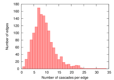
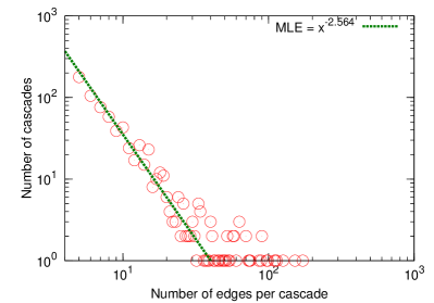
Table 2 shows experimental values of number of cascades that let $E_{1}$ cover different percentages of the edges. To have a closer look at the cascade size distribution, for a Forest Fire network on 1,024 nodes and 1,477 edges, we generated 4,038 cascades. The majority of edges took part in 4 to 12 cascades and the cascade size distribution follows a power law (Figure 5(b)). The average and median number of cascades per edge are 9.1 and 8, respectively (Figure 5(a)).

Type of network	$\bf f$	$\bf|C|$	$\bf r$	BEP	AUC
Forest Fire	0.5	388	2,898	0.393	0.29
	0.9	2,017	14,027	0.75	0.67
	0.95	2,717	19,418	0.82	0.74
	0.99	4,038	28,663	0.92	0.86
Hierarchical Kronecker	0.5	289	1,341	0.37	0.30
	0.9	1,209	5,502	0.81	0.80
	0.95	1,972	9,391	0.90	0.90
	0.99	5,078	25,643	0.98	0.98
Core-periphery Kronecker	0.5	140	1,392	0.31	0.23
	0.9	884	9,498	0.84	0.80
	0.95	1,506	14,125	0.93	0.91
	0.99	3,110	30,453	0.98	0.96
Flat Kronecker	0.5	200	1,324	0.34	0.26
	0.9	1,303	7,707	0.84	0.83
	0.95	1,704	9,749	0.89	0.88
	0.99	3,652	21,153	0.97	0.97

Table 2: Performance of synthetic data. Break-even Point (BEP) and Receiver Operating Characteristic (AUC) when we generated the minimum number of $|C|$ cascades so that $f$-fraction of edges participated in at least one cascades $|E_{l}|\geq f|E|$. These $|C|$ cascades generated the total of $r$ edge transmissions, i.e., average cascade size is $r/|C|$. All networks have 1,024 nodes and 1,446 edges. We use the exponential incubation time model with parameter $\alpha=1$, and in each case we set the probability $\beta$ such that $r/|C|$ is neither too small nor too large (i.e., $\beta\in(0.1,0.6)$).

Baseline method. To infer a diffusion network $\hat{G}$, we consider the a simple baseline heuristic where we compute the score of each edge and then pick $k$ edges with highest score.

More precisely, for each possible edge $(u,v)$ of $G$, we compute $w(u,v)=\sum_{c\in C}P_{c}(u,v)$, i.e., overall how likely were the cascades $c\in C$ to propagate over the edge $(u,v)$. Then we simply pick the $k$ edges $(u,v)$ with the highest score $w(u,v)$ to obtain $\hat{G}$. For example, Figure 1(b) shows the results of the baseline method on a small graph.

Solution quality. We evaluate the performance of the NetInf algorithm in two different ways. First, we are interested in how successful NetInf is at optimizing the objective function $F_{C}(G)$ that is NP-hard to optimize exactly. Using the online bound in Theorem 3.8, we can assess at most how far from the unknown optimal the NetInf solution is in terms of the log-likelihood score. Second, we also evaluate the NetInf based on accuracy, i.e., what fraction of edges of $G^{*}$ NetInf managed to infer correctly.

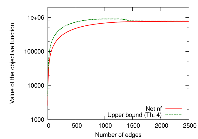
Figure 6(a) plots the value of the log-likelihood improvement $F_{C}(G)$ as a function of the number of edges in $G$. In red we plot the value achieved by NetInf and in green the upper bound using Theorem 3.8. The plot shows that the value of the unknown optimal solution (that is NP-hard to compute exactly) is somewhere between the red and the green curve. Notice that the band between two curves, the optimal and the NetInf curve, is narrow. For example, at 2,000 edges in $\hat{G}$, NetInf finds the solution that is least 97% of the optimal graph. Moreover, also notice a strong diminishing return effect. The value of the objective function flattens out after about 1,000 edges. This means that, in practice, very sparse solutions (almost tree-like diffusion graphs) already achieve very high values of the objective function close to the optimal.

(a) Kronecker network

(b) Real MemeTracker data

Figure 6: Score achieved by NetInf in comparison with the online upper bound from Theorem 3.8. In practice NetInf finds networks that are at 97% of NP-hard to compute optimal.

Accuracy of NetInf. We also evaluate our approach by studying how many edges inferred by NetInf are actually present in the true network $G^{*}$. We measure the precision and recall of our method. For every value of $k$ ($1\leq k\leq n(n-1)$) we generate $\hat{G_{k}}$ on $k$ edges by using NetInf or the baseline method. We then compute precision (which fraction of edges in $\hat{G_{k}}$ is also present $G^{*}$) and recall (which fraction of edges of $G^{*}$ appears in $\hat{G_{k}}$). For small $k$, we expect low recall and high precision as we select the few edges that we are the most confident in. As $k$ increases, precision will generally start to drop but the recall will increase.

(a) Hier. Kronecker (Exp)

(b) Core-Periph. Kronecker (Exp)

(c) Flat Kronecker (Exp)

(d) Hier. Kronecker (PL)

(e) Core-Periph. Kronecker (PL)

(f) Flat Kronecker (PL)

(g) Forest Fire (PL, $\alpha=1.1$)

(h) Forest Fire (PL, $\alpha=3$)

Figure 7: Precision and recall for three 1024 node Kronecker and Forest Fire network networks with exponential (Exp) and power law (PL) incubation time model. The plots are generated by sweeping over values of $k$, that controls the sparsity of the solution.

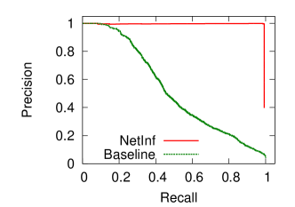
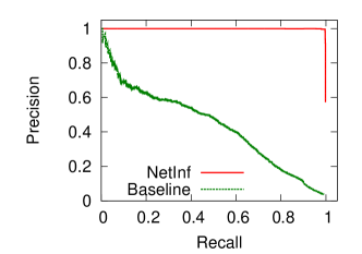
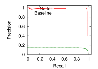
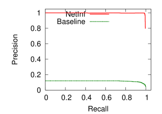
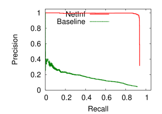
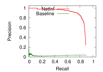
Figure 7 shows the precision-recall curves of NetInf and the baseline method on three different Kronecker graphs (random, hierarchical community structure and core-periphery structure) with 1024 nodes and two incubation time models. The cascades were generated with an exponential incubation time model with $\alpha=1$, or a power law incubation time model with $\alpha=2$ and a value of $\beta$ low enough to avoid generating too large cascades (in all cases, we pick a value of $\beta\in(0.1,0.6)$). For each network we generated between 2,000 and 4,000 cascades so that 99% of the edges of $G^{*}$ participated in at least one cascade. We chose cascade starting points uniformly at random.

First, we focus on Figures 7(a), 7(b) and 7(c) where we use the exponential incubation time model on different Kronecker graphs. Notice that the baseline method achieves the break-even point between 0.4 and 0.5 on all three networks. On the other hand, NetInf performs much better with the break-even point of 0.99 on all three datasets.

We view this as a particularly strong result as we were especially careful not to generate too many cascades since more cascades mean more evidence that makes the problem easier. Thus, using a very small number of cascades, where every edge of $G^{*}$ participates in only a few cascades, we can almost perfectly recover the underlying diffusion network $G^{*}$. Second important point to notice is that the performance of NetInf seems to be strong regardless of the structure of the network $G^{*}$. This means that NetInf works reliably regardless of the particular structure of the network of which contagions propagated (refer to Table 2).

Similarly, Figures 7(d), 7(e) and 7(f) show the performance on the same three networks but using the power law incubation time model. The performance of the baseline now dramatically drops. This is likely due to the fact that the variance of power-law (and heavy tailed distributions in general) is much larger than the variance of an exponential distribution. Thus the diffusion network inference problem is much harder in this case. As the baseline pays high price due to the increase in variance with the break-even point dropping below $0.1$ the performance of NetInf remains stable with the break even point in the high 90s.

Figure 8: Performance of NetInf as a function of the amount of cascade data. The units in the x-axis are normalized. $x=1$ means that the total number of transmission events used for the experiment was equal to the number of edges in $G^{*}$. On average NetInf requires about two propagation events per edge of the original network in order to reliably recover the true network structure.

We also examine the results on the Forest Fire network (Figures 7(g) and 7(h)). Again, the performance of the baseline is very low while NetInf achieves the break-even point at around 0.90.

Generally, the performance on the Forest Fire network is a bit lower than on the Kronecker graphs. However, it is important to note that while these networks have very different global network structure (from hierarchical, random, scale free to core periphery) the performance of NetInf is remarkably stable and does not seem to depend on the structure of the network we are trying to infer or the particular type of cascade incubation time model.

Finally, in all the experiments, we observe a sharp drop in precision for high values of recall (near $1$). This happens because the greedy algorithm starts to choose edges with low marginal gains that may be false edges, increasing the probability to make mistakes.

Performance vs. cascade coverage. Intuitively, the larger the number of cascades that spread over a particular edge the easier it is to identify it. On one hand if the edge never transmitted then we can not identify it, and the more times it participated in the transmission of a contagion the easier should the edge be to identify.

In our experiments so far, we generated a relatively small number of cascades. Next, we examine how the performance of NetInf depends on the amount of available cascade data. This is important because in many real world situations the data of only a few different cascades is available.

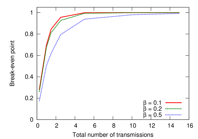
Figure 8 plots the break-even point of NetInf as a function of the available cascade data measured in the number of contagion transmission events over all cascades. The total number of contagion transmission events is simply the sum of cascade sizes. Thus, $x=1$ means that the total number of transmission events used for the experiment was equal to the number of edges in $G^{*}$. Notice that as the amount of cascade data increases the performance of NetInf also increases. Overall we notice that NetInf requires a total number of transmission events to be about 2 times the number of edges in $G^{*}$ to successfully recover most of the edges of $G^{*}$.

Moreover, the plot shows the performance for different values of edge transmission probability $\beta$. As noted before, big values of $\beta$ produce larger cascades. Interestingly, when cascades are small (small $\beta$) NetInf needs less data to infer the network than when cascades are larger. This occurs because the larger a cascade, the more difficult is to infer the parent of each node, since we have more potential parents for each the node to choose from. For example, when $\beta=0.1$ NetInf needs about $2|E|$ transmission events, while when $\beta=0.5$ it needs twice as much data (about $4|E|$ transmissions) to obtain the break even point of $0.9$.

Figure 9: Average time per edge added by our algorithm implemented with lazy evaluation (LE) and localized update (LU).

Stopping criterion. In practice one does not know how long to run the algorithm and how many edges to insert into the network $\hat{G}$. Given the results from Figure 6, we found the following heuristic to give good results. We run the NetInf algorithm for $k$ steps where $k$ is chosen such that the objective function is “close” to the upper bound, i.e., $F_{C}(\hat{G})>x\cdot\textrm{OPT}$, where OPT is obtained using the online bound. In practice we use values of $x$ in range $0.8$–$0.9$. That means that in each iteration $k$, OPT is computed by evaluating the right hand side expression of the equation in Theorem 3.8, where $k$ is simply the iteration number. Therefore, OPT is computed online, and thus the stopping condition is also updated online.

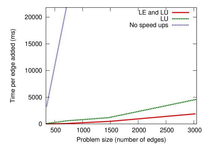
Scalability. Figure 9 shows the average computation time per edge added for the NetInf algorithm implemented with lazy evaluation and localized update. We use a hierarchical Kronecker network and an exponential incubation time model with $\alpha=1$ and $\beta=0.5$. Localized update speeds up the algorithm for an order of magnitude (45$\times$) and lazy evaluation further gives a factor of 6 improvement. Thus, overall, we achieve two orders of magnitude speed up (280$\times$), without any loss in solution quality.

In practice the NetInf algorithm can easily be used to infer networks of 10,000 nodes in a matter of hours.

Figure 10: Break-even point of NetInf as a function of the amount of additive Gaussian noise in the incubation time.

Performance vs. incubation time noise. In our experiments so far, we have assumed that the incubation time values between infections are not noisy and that we have access to the true distribution from which the incubation times are drawn. However, real data may violate any of these two assumptions.

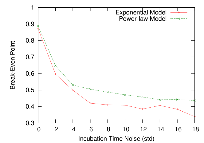
We study the performance of NetInf (break-even point) as a function of the noise of the waiting time between infections. Thus, we add Gaussian noise to the waiting times between infections in the cascade generation process.

Figure 10 plots the performance of NetInf (break-even point) as a function of the amount of Gaussian noise added to the incubation times between infections for both an exponential incubation time model with $\alpha=1$, and a power law incubation time model with $\alpha=2$. The break-even point degrades with noise but once a high value of noise is reached, an additional increment in the amount of noise does not degrade further the performance of NetInf. Interestingly, the break-even point value for high values of noise is very similar to the break-even point achieved later in a real dataset (Figures 13(a) and 13(b)).

Performance vs. infections by the external source. In all our experiments so far, we have assumed that we have access to complete cascade data, i.e., we are able to observe all the nodes taking part in each cascade. Thereby, except for the first node of a cascade, we do not have any “jumps” or missing nodes in the cascade as it spreads across the network. Even though techniques for coping with missing data in information cascades have recently been investigated [Sadikov et al. (2011)], we evaluate NetInf against both scenarios.

(a) Missing node infection data

(b) Node infections due to external source

Figure 11: Break-even point of NetInf as (a) function of the fraction of missing nodes per cascade, and as (b) function of the fraction of nodes that are infected by an external source per cascade.

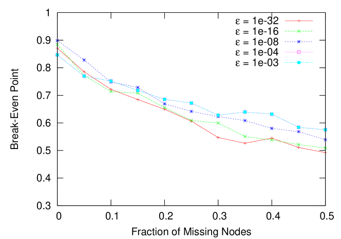
First, we consider the case where a random fraction of each cascade is missing. This means that we first generate a set of cascades, but then only record node infection times of $f$-fraction of nodes. We first generate enough cascades so that without counting the missing nodes in the cascades, we still have that 99% of the edges in $G^{*}$ participate in at least one cascade. Then we randomly delete (i.e., set infection times to infinity) $f$-fraction of nodes in each cascade.

Figure 11(a) plots the performance of NetInf (break-even point) as a function of the percentage of missing nodes in each cascade. Naturally, the performance drops with the amount of missing data. However, we also note that the effect of missing nodes can be mitigated by an appropriate choice of the parameter $\varepsilon$. Basically, higher $\varepsilon$ makes propagation via $\varepsilon$-edges more likely and thus by giving a cascade a greater chance to propagate over the $\varepsilon$-edges NetInf can implicitly account for the missing data.

Second, we also consider the case where the contagion does not spread through the network via diffusion but rather due to the influence of an external source. Thus, the contagion does not really spread over the edges of the network but rather appears almost at random at various nodes of the network.

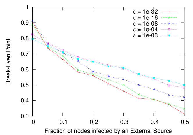
Figure 11(b) plots the performance of NetInf (break-even point) as a function of the percentage of nodes that are infected by an external source for different values of $\varepsilon$. In our framework, we model the influence due to the external source with the $\varepsilon$-edges. Note that appropriately setting $\varepsilon$ can appropriately account for the exogenous infections that are not the result of the network diffusion but due to the external influence. The higher the value of $\varepsilon$, the stronger the influence of the external source, i.e., we assume a greater number of missing nodes or number of nodes that are infected by an external source. Thus, the break-even is more robust for higher values of $\varepsilon$.

Figure 12: Hyperlink-based cascades versus meme-based cascades. In hyper-link cascades, if post $j$ linked to post $k$, we consider this as a contagion transmission event with the post creation time as the corresponding infection time. In MemeTracker cascades, we follow the spread of a short textual phrase and use post creation times as infection times.

4.2 Experiments on real data

Dataset description. We use more than $172$ million news articles and blog posts from $1$ million online sources over a period of one year from September 1 2008 till August 31 2009. Based on this raw data, we use two different methodologies to trace information on the Web and then create two different datasets:

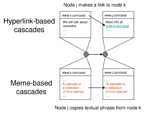
(1) Blog hyperlink cascades dataset: We use hyperlinks between blog posts to trace the flow of information [Leskovec et al. (2007)]. When a blog publishes a piece of information and uses hyper-links to refer to other posts published by other blogs we consider this as events of information transmission. A cascade $c$ starts when a blog publishes a post $P$ and the information propagates recursively to other blogs by them linking to the original post or one of the other posts from which we can trace a chain of hyperlinks all the way to the original post $P$ . By following the chains of hyperlinks in the reverse direction we identify hyperlink cascades [Leskovec et al. (2007)]. A cascade is thus composed of the time-stamps of the hyperlink/post creation times.

(1) MemeTracker dataset: We use the MemeTracker [Leskovec et al. (2009)] methodology to extract more than 343 million short textual phrases (like, “Joe, the plumber” or “lipstick on a pig”). Out of these, 8 million distinct phrases appeared more than 10 times, with the cumulative number of mentions of over 150 million. We cluster the phrases to aggregate different textual variants of the same phrase [Leskovec et al. (2009)]. We then consider each phrase cluster as a separate cascade $c$. Since all documents are time stamped, a cascade $c$ is simply a set of time-stamps when blogs first mentioned phrase $c$. So, we observe the times when blogs mention particular phrases but not where they copied or obtained the phrases from. We consider the largest 5,000 cascades (phrase clusters) and for each website we record the time when they first mention a phrase in the particular phrase cluster. Note that cascades in general do not spread over all the sites, which our methodology can successfully handle.

Figure 12 further illustrates the concept of hyper-link and MemeTracker cascades.

(a) Blog hyperlink cascades dataset

(b) MemeTracker dataset

Figure 13: Precision and recall for a 500 node hyperlink network using (a) the blog hyperlink cascades dataset (i.e., hyperlinks cascades) and (b) the MemeTracker dataset (i.e., MemeTracker cascades). We used $\beta=0.5$, $\varepsilon=10^{-9}$ and the exponential model with $\alpha=1.0$. The time units were hours.

Accuracy on real data. As there is not ground truth network for both datasets, we use the following way to create the ground truth network $G^{*}$. We create a network where there is a directed edge $(u,v)$ between a pair of nodes $u$ and $v$ if a post on site $u$ linked to a post on site $v$. To construct the network we take the top 500 sites in terms of number of hyperlinks they create/receive. We represent each site as a node in $G^{*}$ and connect a pair of nodes if a post in first site linked to a post in the second site. This process produces a ground truth network $G^{*}$ with 500 nodes and 4,000 edges.

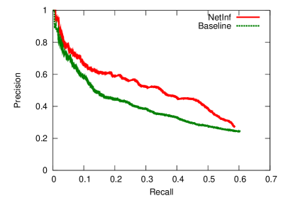
First, we use the blog hyperlink cascades dataset to infer the network $\hat{G}$ and evaluate how many edges NetInf got right. Figure 13(a) shows the performance of NetInf and the baseline. Notice that the baseline method achieves the break-even point of 0.34, while our method performs better with a break-even point of 0.44, almost a 30% improvement.

Figure 14: Small part of a news media (red) and blog (blue) diffusion network. We use the blog hyperlink cascades dataset, i.e., hyperlinks between blog and news media posts to trace the flow of information.

NetInf is basically performing a link-prediction task based only on temporal linking information. The assumption in this experiment is that sites prefer to create links to sites that recently mentioned information while completely ignoring the authority of the site. Given such assumption is not satisfied in real-life, we consider the break even point of 0.44 a good result.

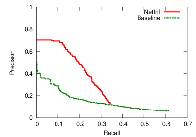
Now, we consider an even harder problem, where we use the Memetracker dataset to infer $G^{*}$. In this experiment, we only observe times when sites mention particular textual phrases and the task is to infer the hyperlink structure of the underlying web graph. Figure 13(b) shows the performance of NetInf and the baseline. The baseline method has a break-even point of 0.17 and NetInf achieves a break-even point of 0.28, more than a 50% improvement

To have a fair comparison with the synthetic cases, notice that the exponential incubation time model is a simplistic assumption for our real dataset, and NetInf can potentially gain additional accuracy by choosing a more realistic incubation time model.

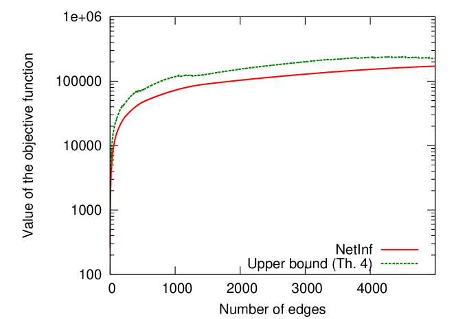
Solution quality. Similarly as with synthetic data, in Figure 6(b) we investigate the value of the objective function and compare it to the online bound. Notice that the bound is almost as tight as in the case of synthetic networks, finding the solution that is least 84% of optimal and both curves are similar in shape to the synthetic case value. Again, as in the synthetic case, the value of the objective function quickly flattens out which means that one needs a relatively few number of edges to capture most of the information flow on the Web.

Figure 15: Small part of a news media (red) and blog (blue) diffusion network. We use the MemeTracker dataset, i.e., textual phrases from MemeTracker to trace the flow of information.

In the remainder of the section, we use the top 1,000 media sites and blogs with the largest number of documents.

Visualization of diffusion networks. We examine the structure of the inferred diffusion networks using both datasets: the blog hyperlink cascades dataset and the MemeTracker dataset.

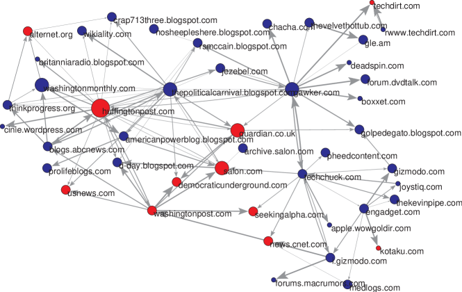
Figure 14 shows the largest connected component of the diffusion network after $100$ edges have been chosen using the first dataset, i.e., using hyperlinks to track the flow of information. The size of the nodes is proportional to the number of articles on the site and the width of the edge is proportional to the probability of influence, i.e., stronger edges have higher width. The strength of an edge across all cascades is simply defined as the marginal gain given by adding the edge in the greedy algorithm (and this is proportional to the probability of influence). Since news media articles rarely use hyperlinks to refer to one another, the network is somewhat biased towards web blogs (blue nodes). There are several interesting patterns to observe.

First, notice that three main clusters emerge: on the left side of the network we can see blogs and news media sites related to politics, at the right top, we have blogs devoted to gossip, celebrity news or entertainment and on the right bottom, we can distinguish blogs and news media sites that deal with technological news. As Huffington Post and Political Carnival play the central role on the political side of the network, mainstream media sites like Washington Post, Guardian and the professional blog Salon.com play the role of connectors between the different parts of the network. The celebrity gossip part of the network is dominated by the blog Gawker and technology news gather around blogs Gizmodo and Engadget, with CNet and TechChuck establishing the connection to the rest of the network.

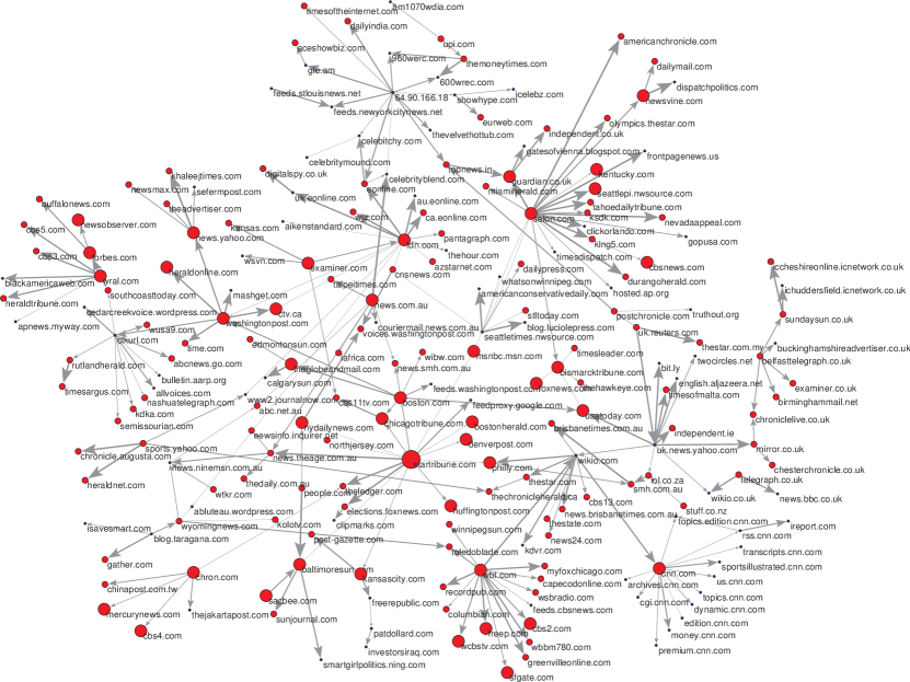
Figure 15 shows the largest connected component of the diffusion network after $300$ edges have been chosen using the second methodology, i.e. using short textual phrases to track the flow of information. In this case, the network is biased towards news media sites due to its higher volume of information.

Insights into the diffusion on the web. The inferred diffusion networks also allow for analysis of the global structure of information propagation on the Web. For this analysis, we use the MemeTracker dataset and analyze the structure of the inferred information diffusion network.

(a) Influence Index

(b) Number of edges as iterations proceed

(c) Median edge time lag

Figure 16: (a) Distribution of node influence index. Most nodes have very low influence (they act as sinks). (b) Number and strength of edges between different media types. Edges of news media influencing blogs are the strongest. (c) Median time lag on edges of different type.

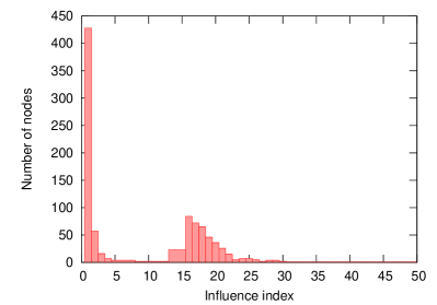
First, Figure 16(a) shows the distribution of the influence index. The influence index is defined as the number of reachable nodes from $w$ by traversing edges of the inferred diffusion network (while respecting edge directions). Nevertheless, we are also interested in the distance from $w$ to its reachable nodes, i.e. nodes at shorter distances are more likely to be infected by $w$. Thus, we slightly modify the definition of influence index to be $\sum_{u}1/d_{wu}$ where we sum over all the reachable nodes from $w$ and $d_{wu}$ is the distance between $w$ and $u$. Notice that we have two types of nodes. There is a small set of nodes that can reach many other nodes, which means they either directly or indirectly propagate information to them. On the other side we have a large number of sites that only get influenced but do not influence many other sites. This hints at a core periphery structure of the diffusion network with a small set of sites directly or indirectly spreading the information in the rest of the network.

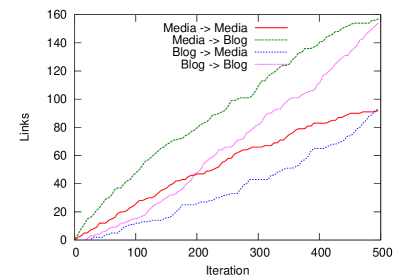
Figure 16(b) investigates the number of links in the inferred network that point between different types of sites. Here we split the sites into mainstream media and blogs. Notice that most of the links point from news media to blogs, which says that most of the time information propagates from the mainstream media to blogs. Then notice how at first many media-to-media links are chosen but in later iterations the increase of these links starts to slow down. This means that media-to-media links tend to be the strongest and NetInf picks them early. The opposite seems to occur in case of blog-to-blog links where relatively few are chosen first but later the algorithm picks more of them. Lastly, links capturing the influence of blogs on mainstream media are the rarest and weakest. This suggests that most information travels from mass media to blogs.

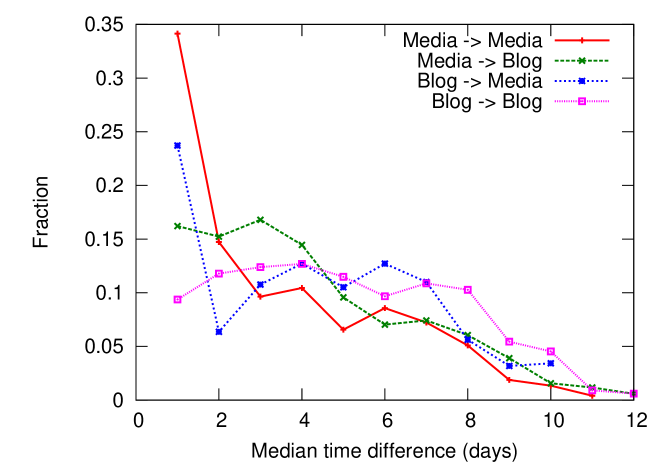
Last, Figure 16(c) shows the median time difference between mentions of different types of sites. For every edge of the inferred diffusion network, we compute the median time needed for the information to spread from the source to the destination node. Again, we distinguish the mainstream media sites and blogs. Notice that media sites are quick to infect one another or even to get infected from blogs. However, blogs tend to be much slower in propagating information. It takes a relatively long time for them to get “infected” with information regardless whether the information comes from the mainstream media or the blogosphere.

Finally, we have observed that the insights into diffusion on the web using the inferred network are very similar to insights obtained by simply taking the hyperlink network. However, our aim here is to show that (i) although the quantitative results are modest in terms of precision and recall, the qualitative insights makes sense, and that (ii) it is surprising that using simply timestamps of links, we are able to draw the same qualitative insights as using the hyperlink network

5 Further related work

There are several lines of work we build upon. Although the information diffusion in on-line settings has received considerable attention [Gruhl et al. (2004), Kumar et al. (2004), Adar and Adamic (2005), Leskovec et al. (2006), Leskovec et al. (2006), Leskovec et al. (2007), Liben-Nowell and Kleinberg (2008)], only a few studies were able to study the actual shapes of cascades [Leskovec et al. (2007), Liben-Nowell and Kleinberg (2008), Ghosh and Lerman (2011), Romero et al. (2011), Ver Steeg et al. (2011)]. The problem of inferring links of diffusion was first studied by Adar and Adamic [Adar and Adamic (2005)], who formulated it as a supervised classification problem and used Support Vector Machines combined with rich textual features to predict the occurrence of individual links. Although rich textual features are used, links are predicted independently and thus their approach is similar to our baseline method in the sense that it picks a threshold (i.e., hyperplane in case of SVMs) and predicts individually the most probable links.

The work most closely related to our approach, CoNNIe [Myers and Leskovec (2010)] and NetRate [Gomez-Rodriguez et al. (2011)], also uses a generative probabilistic model for the problem of inferring a latent social network from diffusion (cascades) data. However, CoNNIe and NetRate use convex programming to solve the network inference problem. CoNNIe includes a $l_{1}$-like penalty term that controls sparsity while NetRate provides a unique sparse solution by allowing different transmission rates across edges. For each edge $(i,j)$, CoNNIe infers a prior probability $\beta_{i,j}$ and NetRate infers a transmission rate $\alpha_{i,j}$. Both algorithms are computationally more expensive than NetInf. In our work, we assume that all edges of the network have the same prior probability ($\beta$) and transmission rate ($\alpha$). From this point of view, we think the comparison between the algorithms is unfair since NetRate and CoNNIe have more degrees of freedom

Network structure learning has been considered for estimating the dependency structure of probabilistic graphical models [Friedman and Koller (2003), Friedman et al. (1999)]. However, there are fundamental differences between our approach and graphical models structure learning. (a) we learning directed networks, but Bayes netws are DAGs (b) undirected graphical model structure learning makes no assumption about the network but they learn undirected and we learn directed networks

First, our work makes no assumption about the network structure (we allow cycles, reciprocal edges) and are thus able to learn general directed networks. In directed graphical models, reciprocal edges and cycles are not allowed, and the inferred network is a directed acyclic graph (DAG). In undirected graphical models, there are typically no assumptions about the network structure, but the inferred network is undirected. Second, Bayesian network structure inference methods are generally heuristic approaches without any approximation guarantees. Network structure learning has also been used for estimating epidemiological networks [Wallinga and Teunis (2004)] and for estimating probabilistic relational models [Getoor et al. (2003)]. In both cases, the problem is formulated in a probabilistic framework. However, since the problem is intractable, heuristic greedy hill-climbing or stochastic search that offer no performance guarantee were usually used in practice. In contrast, our work provides a novel formulation and a tractable solution together with an approximation guarantee.

Our work relates to static sparse graph estimation using graphical Lasso methods [Wainwright et al. (2006), Schmidt et al. (2007), Friedman et al. (2008), Meinshausen and Buehlmann (2006)], unsupervised structure network inference using kernel methods [Lippert et al. (2009)], mutual information relevance network inference [Butte and Kohane (2000)], inference of influence probabilities [Goyal et al. (2010)], and extensions to time evolving graphical models [Ahmed and Xing (2009), Ghahramani (1998), Song et al. (2009)]. Our work is also related to a link prediction problem [Jansen et al. (2003), Taskar et al. (2003), Liben-Nowell and Kleinberg (2003), Backstrom and Leskovec (2011), Vert and Yamanishi (2005)] but different in a sense that this line of work assumes that part of the network is already visible to us.

Last, although submodular function maximization has been previously considered for sensor placement [Leskovec et al. (2007)] and finding influencers in viral marketing [Kempe et al. (2003)], to the best of our knowledge, the present work is the first that considers submodular function maximization in the context of network structure learning.

6 Conclusions

We have investigated the problem of tracing paths of diffusion and influence. We formalized the problem and developed a scalable algorithm, NetInf, to infer networks of influence and diffusion. First, we defined a generative model of cascades and showed that choosing the best set of $k$ edges maximizing the likelihood of the data is NP-hard. By exploiting the submodularity of our objective function, we developed NetInf, an efficient algorithm for inferring a near-optimal set of $k$ directed edges. By exploiting localized updates and lazy evaluation, our algorithm is able to scale to very large real data sets.

We evaluated our algorithm on synthetic cascades sampled from our generative model, and showed that NetInf is able to accurately recover the underlying network from a relatively small number of samples. In our experiments, NetInf drastically outperformed a naive maximum weight baseline heuristic.

Most importantly, our algorithm allows us to study properties of real networks. We evaluated NetInf on a large real data set of memes propagating across news websites and blogs. We found that the inferred network exhibits a core-periphery structure with mass media influencing most of the blogosphere. Clusters of sites related to similar topics emerge (politics, gossip, technology, etc.), and a few sites with social capital interconnect these clusters allowing a potential diffusion of information among sites in different clusters.

There are several interesting directions for future work. Here we only used time difference to infer edges and thus it would be interesting to utilize more informative features (e.g., textual content of postings etc.) to more accurately estimate the influence probabilities. Moreover, our work considers static propagation networks, however real influence networks are dynamic and thus it would be interesting to relax this assumption. Last, there are many other domains where our methodology could be useful: inferring interaction networks in systems biology (protein-protein and gene interaction networks), neuroscience (inferring physical connections between neurons) and epidemiology.

We believe that our results provide a promising step towards understanding complex processes on networks based on partial observations.

Acknowledgments

We thank Spinn3r for resources that facilitated the research. The research was supported in part by Albert Yu & Mary Bechmann Foundation, IBM, Lightspeed, Microsoft, Yahoo, grants ONR N00014-09-1-1044, NSF CNS0932392, NSF CNS1010921, NSF IIS1016909, NSF IIS0953413, AFRL FA8650-10-C-7058 and Okawa Foundation Research Grant. Manuel Gomez Rodriguez has been supported in part by a Fundacion Caja Madrid Graduate Fellowship, a Fundacion Barrie de la Maza Graduate Fellowship and by the Max Planck Society.

References

- Adar and Adamic (2005) Adar, E. and Adamic, L. A. 2005. Tracking information epidemics in blogspace. In Web Intelligence. 207–214.
- Adar et al. (2004) Adar, E., Zhang, L., Adamic, L. A., and Lukose, R. M. 2004. Implicit structure and the dynamics of blogspace. In Workshop on the Weblogging Ecosystem.
- Ahmed and Xing (2009) Ahmed, A. and Xing, E. 2009. Recovering time-varying networks of dependencies in social and biological studies. In PNAS ’09: Proceedings of the National Academy of Sciences. Vol. 106.
- Anderson and May (2002) Anderson, R. M. and May, R. M. 2002. Infectious diseases of humans: Dynamics and control. Oxford Press.
- Backstrom and Leskovec (2011) Backstrom, L. and Leskovec, J. 2011. Supervised random walks: Predicting and recommending links in social networks. In WSDM ’11: Proceedings of the ACM International Conference on Web Search and Data Mining.
- Bailey (1975) Bailey, N. T. J. 1975. The Mathematical Theory of Infectious Diseases and its Applications, 2nd ed. Hafner Press.
- Barabási (2005) Barabási, A.-L. 2005. The origin of bursts and heavy tails in human dynamics. Nature 435, 207.
- Barabási and Albert (1999) Barabási, A.-L. and Albert, R. 1999. Emergence of scaling in random networks. Science 286, 509–512.
- Butte and Kohane (2000) Butte, A. and Kohane, I. 2000. Mutual information relevance networks: functional genomic clustering using pairwise entropy measurements. In Pac Symp Biocomput. Vol. 5. 418–429.
- Clauset et al. (2008) Clauset, A., Moore, C., and Newman, M. E. J. 2008. Hierarchical structure and the prediction of missing links in networks. Nature 453, 7191, 98–101.
- Crane and Sornette (2008) Crane, R. and Sornette, D. 2008. Robust dynamic classes revealed by measuring the response function of a social system. PNAS ’08: Proceedings of the National Academy of Sciences 105, 41 (October), 15649–15653.
- Domingos and Richardson (2001) Domingos, P. and Richardson, M. 2001. Mining the network value of customers. In KDD ’01: Proceedings of the 7th ACM SIGKDD international conference on Knowledge discovery and data mining.
- Edmonds (1967) Edmonds, J. 1967. Optimum branchings. Journal of Research of the National Bureau of Standards 71B, 233–240.
- Erdős and Rényi (1960) Erdős, P. and Rényi, A. 1960. On the evolution of random graphs. Publication of the Mathematical Institute of the Hungarian Academy of Science 5, 17–67.
- Friedman et al. (2008) Friedman, J., Hastie, T., and Tibshirani, R. 2008. Sparse inverse covariance estimation with the graphical lasso. Biostat 9, 3, 432–441.
- Friedman and Koller (2003) Friedman, N. and Koller, D. 2003. Being Bayesian about network structure. A Bayesian approach to structure discovery in Bayesian networks. Machine Learning 50, 1, 95–125.
- Friedman et al. (1999) Friedman, N., Nachman, I., and Pe’er, D. 1999. Learning Bayesian network structure from massive datasets: The “Sparse Candidate” algorithm. In UAI ’99: Proceedings of the 15th Conference on Uncertainty in Artificial Intelligence.
- Getoor et al. (2003) Getoor, L., Friedman, N., Koller, D., and Taskar, B. 2003. Learning probabilistic models of link structure. The Journal of Machine Learning Research 3, 707.
- Ghahramani (1998) Ghahramani, Z. 1998. Learning dynamic Bayesian networks. In Adaptive Processing of Sequences and Data Structures.
- Ghosh and Lerman (2011) Ghosh, R. and Lerman, K. 2011. A framework for quantitative analysis of cascades on networks. In WSDM ’11: Proceedings of the fourth ACM international conference on Web search and data mining. 665–674.
- Gomez-Rodriguez et al. (2011) Gomez-Rodriguez, M., Balduzzi, D., and Schölkopf, B. 2011. Uncovering the Temporal Dynamics of Diffusion Networks. In ICML ’11: Proceedings of the 28th International Conference on Machine Learning. 561–568.
- Goodman (1961) Goodman, L. A. 1961. Snowball sampling. Annals of Mathematical Statistics 32, 1, 148–170.
- Goyal et al. (2010) Goyal, A., Bonchi, F., and Lakshmanan, L. 2010. Learning influence probabilities in social networks. In WSDM ’10: Proceedings of the Third ACM International Conference on Web Search and Data Mining. ACM, 241–250.
- Gruhl et al. (2004) Gruhl, D., Guha, R., Liben-Nowell, D., and Tomkins, A. 2004. Information diffusion through blogspace. In WWW ’04: Proceedings of the 13th international conference on World Wide Web. 491–501.
- Heckathorn (1997) Heckathorn, D. 1997. Respondent-driven sampling: A new approach to the study of hidden populations. Social Problems 44, 2, 174–199.
- Hethcote (2000) Hethcote, H. W. 2000. The mathematics of infectious diseases. SIAM Review 42, 4, 599–653.
- Jansen et al. (2003) Jansen, R., Yu, H., Greenbaum, D., Kluger, Y., Krogan, N., Chung, S., Emili, A., Snyder, M., Greeblatt, J., and Gerstein, M. 2003. A bayesian networks approach for predicting proteinprotein interactions from genomic data. Science 302, 5644, 449–453.
- Katz and Lazarsfeld (1955) Katz, E. and Lazarsfeld, P. 1955. Personal influence: The part played by people in the flow of mass communications. Free Press.
- Kearns et al. (2006) Kearns, M., Suri, S., and Montfort, N. 2006. An experimental study of the coloring problem on human subject networks. Science 313, 5788, 824.
- Kempe et al. (2003) Kempe, D., Kleinberg, J. M., and Tardos, E. 2003. Maximizing the spread of influence through a social network. In KDD ’03: Proceedings of the 9th ACM SIGKDD international conference on Knowledge discovery and data mining. 137–146.
- Khuller et al. (1999) Khuller, S., Moss, A., and Naor, J. 1999. The budgeted maximum coverage problem. Information Processing Letters 70, 1, 39–45.
- Knuth (1968) Knuth, D. 1968. The art of computer programming. Addison-Wesley.
- Kumar et al. (2004) Kumar, R., Novak, J., Raghavan, P., and Tomkins, A. 2004. Structure and evolution of blogspace. CACM 47, 12, 35–39.
- Leskovec et al. (2006) Leskovec, J., Adamic, L. A., and Huberman, B. A. 2006. The dynamics of viral marketing. In EC ’06: Proceedings of the 7th ACM conference on Electronic commerce. 228–237.
- Leskovec et al. (2009) Leskovec, J., Backstrom, L., and Kleinberg, J. 2009. Meme-tracking and the dynamics of the news cycle. In KDD ’09: Proceedings of the 15th ACM SIGKDD international conference on Knowledge discovery and data mining. ACM, New York, NY, USA, 497–506.
- Leskovec and Faloutsos (2007) Leskovec, J. and Faloutsos, C. 2007. Scalable modeling of real graphs using kronecker multiplication. In ICML ’07: Proceedings of the 24th International Conference on Machine Learning. 504.
- Leskovec et al. (2005) Leskovec, J., Kleinberg, J., and Faloutsos, C. 2005. Graphs over time: densification laws, shrinking diameters and possible explanations. In KDD ’05: Proceedings of the 11th ACM SIGKDD international conference on Knowledge discovery in data mining. 187.
- Leskovec et al. (2007) Leskovec, J., Kleinberg, J. M., and Faloutsos, C. 2007. Graph evolution: Densification and shrinking diameters. ACM Transactions on Knowledge Discovery from Data (TKDD) 1, 1, 2.
- Leskovec et al. (2007) Leskovec, J., Krause, A., Guestrin, C., Faloutsos, C., VanBriesen, J., and Glance, N. 2007. Cost-effective outbreak detection in networks. In KDD ’07: Proceedings of the 13th ACM SIGKDD international conference on Knowledge discovery and data mining. 420–429.
- Leskovec et al. (2008) Leskovec, J., Lang, K. J., Dasgupta, A., and Mahoney, M. W. 2008. Statistical properties of community structure in large social and information networks. In WWW ’08: Proceedings of the 17th International Conference on World Wide Web.
- Leskovec et al. (2007) Leskovec, J., McGlohon, M., Faloutsos, C., Glance, N., and Hurst, M. 2007. Cascading behavior in large blog graphs. In SDM ’07: Proceedings of the SIAM Conference on Data Mining.
- Leskovec et al. (2006) Leskovec, J., Singh, A., and Kleinberg, J. M. 2006. Patterns of influence in a recommendation network. In PAKDD ’06: Proceedings of the 10th Pacific-Asia Conference on Knowledge Discovery and Data Mining. 380–389.
- Liben-Nowell and Kleinberg (2003) Liben-Nowell, D. and Kleinberg, J. 2003. The link prediction problem for social networks. In CIKM ’03: Proceedings of the International Conference on Information and Knowledge Management. 556–559.
- Liben-Nowell and Kleinberg (2008) Liben-Nowell, D. and Kleinberg, J. 2008. Tracing the flow of information on a global scale using Internet chain-letter data. PNAS ’08: Proceedings of the National Academy of Sciences 105, 12 (25 Mar.), 4633–4638.
- Lippert et al. (2009) Lippert, C., Stegle, O., Ghahramani, Z., and Borgwardt, K. 2009. A kernel method for unsupervised structured network inference. In AISTATS ’09: Proceedings of the Artificial Intelligence and Statistics.
- Malmgren et al. (2008) Malmgren, R. D., Stouffer, D. B., Motter, A. E., and Amaral, L. A. A. N. 2008. A poissonian explanation for heavy tails in e-mail communication. Proceedings of the National Academy of Sciences 105, 47 (November), 18153–18158.
- Meinshausen and Buehlmann (2006) Meinshausen, N. and Buehlmann, P. 2006. High-dimensional graphs and variable selection with the lasso. The Annals of Statistics, 1436–1462.
- Myers and Leskovec (2010) Myers, S. and Leskovec, J. 2010. On the Convexity of Latent Social Network Inference. In NIPS ’10: Advances in Neural Information Processing Systems.
- Nemhauser et al. (1978) Nemhauser, G., Wolsey, L., and Fisher, M. 1978. An analysis of approximations for maximizing submodular set functions. Mathematical Programming 14, 1, 265–294.
- Rogers (1995) Rogers, E. M. 1995. Diffusion of Innovations, Fourth ed. Free Press, New York.
- Romero et al. (2011) Romero, D., Meeder, B., and Kleinberg, J. 2011. Differences in the mechanics of information diffusion across topics: Idioms, political hashtags, and complex contagion on twitter. In WWW ’11: Proceedings of the 20th international conference on World wide web. ACM, 695–704.
- Sadikov et al. (2011) Sadikov, S., Medina, M., Leskovec, J., and Garcia-Molina, H. 2011. Correcting for missing data in information cascades. In WSDM ’11: Proceedings of the ACM International Conference on Web Search and Data Mining.
- Schmidt et al. (2007) Schmidt, M., Niculescu-Mizil, A., and Murphy, K. 2007. Learning graphical model structure using l1-regularization paths. In AAAI ’07: Proceedings of the 21th Conference on Artificial Intelligence. Vol. 22.
- Song et al. (2009) Song, L., Kolar, M., and Xing, E. 2009. Time-varying dynamic bayesian networks. In NIPS ’09: Advances in Neural Information Processing Systems.
- Strang and Soule (1998) Strang, D. and Soule, S. A. 1998. Diffusion in organizations and social movements: From hybrid corn to poison pills. Annual Review of Sociology 24, 265–290.
- Taskar et al. (2003) Taskar, B., Wong, M. F., Abbeel, P., and Koller, D. 2003. Link prediction in relational data. In NIPS ’03: Advances in Neural Information Processing Systems.
- Tutte (1948) Tutte, W. 1948. The disection of equilateral triangles into equilateral triangles. Proceedings Cambridge Philos. Soc. 44, 463–482.
- Ver Steeg et al. (2011) Ver Steeg, G., Ghosh, R., and Lerman, K. 2011. What stops social epidemics? In ICWSM ’11: Proceedings of the 5th Int. Conf. on Weblogs and Social Media.
- Vert and Yamanishi (2005) Vert, J. and Yamanishi, Y. 2005. Supervised graph inference. In NIPS ’05: Advances in Neural Information Processing Systems.
- Wainwright et al. (2006) Wainwright, M. J., Ravikumar, P., and Lafferty, J. D. 2006. High-dimensional graphical model selection using ‘1-regularized logistic regression. In PNAS ’06: Proceedings of the National Academy of Sciences.
- Wallinga and Teunis (2004) Wallinga, J. and Teunis, P. 2004. Different epidemic curves for severe acute respiratory syndrome reveal similar impacts of control measures. American Journal of Epidemiology 160, 6, 509–516.
- Watts and Dodds (2007) Watts, D. J. and Dodds, P. S. 2007. Influentials, networks, and public opinion formation. Journal of Consumer Research 34, 4 (December), 441–458.