Partonic Interpretation of Generalized Parton Distributions

Abstract

Generalized Parton Distributions describe, within QCD factorization, the non perturbative component in the amplitudes for deeply virtual exclusive processes. However, in order for a partonic interpretation to hold, semi-disconnected diagrams should not contribute. We show that this condition is not satisfied for non-forward kinematics at leading order, and that gluon mediated re-interactions are essential for a consistent description in terms of parton degrees of freedom.

Generalized Parton Distributions (GPDs) are defined as extensions of the parton distributions from Deep Inelastic Scattering (DIS) to a more complex phase space domain where off-diagonal matrix elements can be related to the partons displacements in transverse space. As a consequence of the factorization theorem of QCD Ji , GPDs enter the matrix elements for the Deeply Virtual Compton Scattering (DVCS) amplitudes. Because the momenta of the outgoing and incoming quark and proton are different, two distinct kinematical regions can be defined. By denoting $X=k^{+}/P^{+}$ the light cone momentum fraction of the struck quark relative to the initial proton momentum, $P^{+}$, and by $X-\zeta=k^{\prime+}/P^{+}$ the corresponding momentum fraction of the returning quark ($\zeta=\Delta^{+}/P^{+}$ represents the t-channel momentum transfer fraction), two distinct regions appear. In the $X>\zeta$ region both the struck and returning quark carry positive momentum fractions of the initial proton momentum. This is called the Dokshitzer-Gribov-Lipatov-Altarelli-Parisi (DGLAP) region because of the way parton evolution is expected to proceed.

The $X<\zeta$ region has been interpreted as describing a quark-antiquark pair emerging from the proton, more similar to the generalization of a distribution amplitude. Evolution proceeds through the Efremov-Radyushkin-Brodsky-Lepage (ERBL) mechanism.

This way of interpreting the ERBL region was proposed at the inception of DVCS studies. In GolLiu_disp we found a reason of concern in noticing that it imposes several seemingly artificial constraints for partonic based descriptions and model building. In particular, symmetry requirements under $X\rightarrow-X$ follow for charge conjugation, $C$, even or odd combinations of parton distributions. These violate the standard Kuti-Weisskopf separation of valence (flavor non singlet) and sea (flavor singlet) quarks, and they may not be naturally satisfied in a large class of models including all spectator models AHLT ; BroEst ; Metz . An even more compelling issue examined here is whether the ERBL region relates at all to the proton’s partonic substructure. In order to prove this, one has to ascertain that the quark anti-quark pair emerges directly from the proton, rather than being a vacuum hadronic fluctuation. Three conditions are essential to characterize a partonic description Jaffe :

1. the support in $X$ is defined by the region $\mid X\mid\leq 1$;

2. analytic properties of the partonic amplitude have to correspond to the emission and absorption of quarks/antiquarks via well defined on-mass shell intermediate hadronic states;

3. the quark-proton vertices have to be connected.

A careful derivation of the parton model from the connected matrix elements for the non-local quark and gluon fields operators that enter inclusive hard processes was given in Jaffe (a formal extension to the off-forward case was given in Die_Gou ). There it was pointed out that a “simple” physical picture does not emerge uniquely and naturally from the structure of the correlator, but that analytic properties need to be taken into consideration.

We now extend the arguments of Jaffe to the ERBL region that similarly presents a more complicated partonic structure. A factorized form was derived in Ref.Ji (for a review see Diehl_rev ) for the DVCS amplitude as

$$\mathcal{F} = \int\limits_{-\zeta+1}^{1}dX\left(\frac{1}{X-\zeta+i\epsilon}-\frac{1}{X+i\epsilon}\right)$$ (1)

$$\times \int dz^{-}e^{i\,q^{+}z^{-}}\langle P^{\prime}\mid\bar{\psi}(z^{-})\gamma^{+}\psi(0)\mid P\rangle.$$

The matrix element in the equation corresponds to GPDs defined e.g. in the unpolarized case as

$$\int dz^{-}e^{i\,q^{+}z-}\langle P^{\prime}\mid\bar{\psi}(z^{-})\gamma^{+}\psi(0)\mid P\rangle=$$

$$\overline{U}(P^{\prime})\left[H(X,\zeta,t)\,\gamma^{+}+E(X,\zeta,t)\,\frac{-i\sigma^{+,\lambda}}{2M}\Delta_{\lambda}\right]U(P)$$ (2)

To clarify the identification of partonic or non-partonic interpretations of the GPDs we can explicitly expand the quark field operators of Eq.(Partonic Interpretation of Generalized Parton Distributions) in terms of light front free field variables (implicitly employing the operator product expansion as in Ref. Jaffe ). We use the decomposition into creation and annihilation operators focusing for simplicity on $H$, as Diehl_rev

$$H(X,\zeta,t)=\frac{1}{2\bar{P}^{+}}\sum_{\lambda}\int\frac{d^{2}k_{T}}{2\sqrt{\mid X^{2}-\zeta^{2}\mid}(2\pi)^{3}}$$

$$\left[\langle P^{\prime}|b_{\lambda}^{\dagger}\,(X-\zeta,{\bf k}^{\prime}_{T})\>b_{\lambda}\,(X,{\bf k}_{T})|P\rangle\>\right.$$

$$+\;\langle P^{\prime}\mid b_{\lambda}^{\dagger}\,(X-\zeta,-{\bf k}_{T}^{\prime})\>d_{-\lambda}^{\dagger}\,(X,{\bf k}_{T})|P\rangle$$

$$+\;\langle P^{\prime}|d_{\lambda}\,(X-\zeta,-{\bf k}^{\prime}_{T})\>b_{-\lambda}\,(X,{\bf k}_{T})|P\rangle\>$$

$$+\;\left.\langle P^{\prime}|d_{\lambda}\,,(X-\zeta,{\bf k}^{\prime}_{T})\>d_{\lambda}^{\dagger}\,(X,{\bf k}_{T})|P\rangle\>\right].$$ (3)

The relation to possible on-shell intermediate states can be explored by inserting a complete set between the quark field operators acting between the incoming or outgoing proton states. Whether or not the corresponding diagrams contribute depends on the values of $X$ and $\zeta$ and the momenta. It was pointed out by Jaffe Jaffe that even in the forward case, when $\zeta=0$ and $X<0$ there are semi-disconnected contributions to the “unitarity diagrams”, shown in Fig. 1, that do not have a partonic interpretation. However, there are two equivalent forms of the product of the two non-local interacting quark field operators, using the anti-commutation of the operators on the null-plane As a result, from the equivalence of these two forms on can deduce an equivalence between the non-partonic/semi-disconnected diagrams with $X<0$ for quarks and, through the alternative ordering of the fields, a partonic distribution for anti-quarks with $X>0$ represented by the usual connected configuration. The important question here is whether or not this kind of equivalence can be established in the off-forward case in order to allow a partonic interpretation of GPDs.

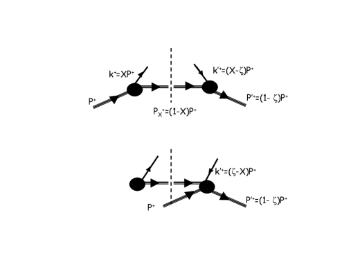
Figure 1: Upper Panel: Parton Model; Lower Panel: Semi-disconnected contribution. The analytic structure of these diagrams was discussed for DIS in Ref.Jaffe .

To consider these questions, insert intermediate states in Eq.(Partonic Interpretation of Generalized Parton Distributions) using completeness, and associate each vertex with plus momentum conservation. In the forward limiting case one obtains

$$H(X,0,0)=\sum_{n}\delta(P^{+}-XP^{+}-P_{n}^{+})\mid\langle n\mid\psi\mid P\rangle\mid^{2}$$ (4)

so for quarks with $X>0$ this corresponds to the usual parton picture in Fig. 1a. For $X<0$ the delta function requires that the intermediate state momentum exceeds the proton $p^{+}$, that is $p_{n}^{+}=P^{+}+|X|p^{+}$. That condition can be satisfied by the creation of a pair from the vacuum as in Fig. 1b, as well as through annihilation of a pair into the vacuum, as shown in detail by Jaffe Jaffe .

Similarly, in the off-forward case

$$H(X,\zeta,t)=\sum_{n}\delta(P^{+}-XP^{+}-P_{n}^{+})\langle P^{\prime}\mid{\bar{\psi}}\mid n\rangle\langle n\mid\psi\mid P\rangle$$ (5)

By expanding $\psi$ and concentrating on the second term in Eq.(Partonic Interpretation of Generalized Parton Distributions) to illustrate the procedure, we have

$$\langle P^{\prime}|d_{\lambda}\,(X-\zeta,-\mbox{\boldmath$k$}^{\prime}_{T})\mid n\rangle\langle n\mid\>b_{-\lambda}\,(X,\mbox{\boldmath$k$}_{T})|P\rangle$$

$$\times\delta(P^{+}-XP^{+}-P_{n}^{+}),$$ (6)

that annihilates a quark with $XP^{+}$ and creates an antiquark with $-(X-\zeta)P^{+}$. For the DGLAP region this cannot conserve plus momentum, but for the ERBL region, $-(X-\zeta)P^{+}$ corresponds to an antiquark. Notice that the delta function has $P_{n}^{+}$ greater than $P^{+}$.

More heuristically, each of the terms in Eq.(Partonic Interpretation of Generalized Parton Distributions) can, on one side describe the processes

$$p\rightarrow q(qq)\;\;\;{\rm and}\;\;\;q(qq)\rightarrow p$$

respectively, at each vertex. The intermediate state $(qq)$ has the quantum numbers of a diquark with momentum $P_{n}$. The equation has a clear partonic interpretation. On the other side, for Eq.(6), consistently with momentum conservation, one has two different types of intermediate states: i) $p\rightarrow q(qqq\bar{q})$ on the LHS, the $\bar{q}$ being re-emitted on the RHS; ii) $p\rightarrow qp(\bar{q})$ on the LHS, the $\bar{q}$ being re-emitted through the semi-disconnected vertex of Fig.1b. In case i) the intermediate state has diquark quantum numbers, a partonic interpretation seems possible but with a catch that we explain in what follows. In case ii) the intermediate state is a $\bar{q}$. The semi-disconnected graphs do not correspond to a partonic description of the proton.

One can show how each of the four terms in Eq. (Partonic Interpretation of Generalized Parton Distributions) corresponds to connected or semi-disconnected graphs. Writing the matrix element for the second term, when $X<\zeta$

$$\langle P^{\prime}\mid b_{\lambda}^{\dagger}\,(X-\zeta,-{\bf k}_{T}^{\prime})|n\rangle\langle n|\>d_{-\lambda}^{\dagger}\,(X,{\bf k}_{T})|P\rangle=$$

$$\langle P^{\prime}\mid b_{\lambda}^{\dagger}\,(X-\zeta,-{\bf k}_{T}^{\prime})|P,n\rangle\langle n|\>d_{-\lambda}^{\dagger}\,(X,{\bf k}_{T})|0\rangle$$ (7)

where the $b^{\dagger}$ has plus momentum $-|X-\zeta|P^{+}$. This corresponds to the Fig. 1b, a “semi-disconnected” graph. In the DIS case, the identification of the initial and final matrix elements in Eq.(4) allows the replacement of the semi-disconnected quark target diagrams for $X<0$ with the connected antiquark-target diagram for $X>0$ (with opposite sign). On the other hand for the GPD, because of the asymmetry between the initial quark-target state and the final state, the semi-disconnected diagrams for $X-\zeta<0$ are equivalent to semi-disconnected diagrams for antiquark-target states, i.e. the ERBL region for quark-target amplitudes is the ERBL region for anti-quark target amplitudes.

Hence, there is a catch that casts a doubt on the possibility of giving a partonic interpretation of the ERBL region. By examining the analytic structure of GPDs, we know that in this region it is either one of the struck quarks/anti-quarks that is put on mass shell BroEst , and not the state with diquark quantum numbers. The only way to have a $\bar{q}$ or equivalently a $q$, as an intermediate is by considering the diagram as in Fig.1b Jaffe , a semi-disconnected, non-partonic contribution. This development contradicts the partonic interpretation of the results for the ERBL region where the Cauchy integration over the quark momentum puts the quark on-shell in the ERBL region, while having an off-shell diquark. In other words, the interpretations of the ERBL region, as would be obtained in Golec ; Die_Gou by inserting different creation and annihilation operators does not address the issue of partonic interpretation. These would require diquark-type states as the intermediate states even in the ERBL region.

In summary, only semi-disconnected graphs contribute to the ERBL region at leading order (Fig.1). These, in turn, do not correspond to partonic distributions. We have a choice. We can take their contribution as $H^{(2)}_{X<\zeta}=0$. Alternatively we can conclude that there are non-partonic contributions to the GPDs and measurements of the ERBL region are not revealing the partonic content of the nucleons, or even the distribution of quark-antiquark meson states in the nucleon.

The impasse in trying to give a partonic interpretation of the ERBL region could be overcome by considering multiparton configurations i.e. extending the definition (Partonic Interpretation of Generalized Parton Distributions) to more than two parton fields. Following Ref.Jaffe one can write diagrams of the type represented in Fig.2. The corresponding analytic structure is given by

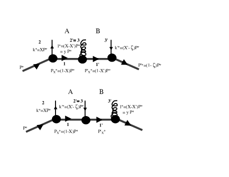
Figure 2: Multiparton contributions to DVCS. Upper panel: a connected one gluon contribution; Lower panel: a connected non planar contribution.

$$H^{(3)}(X,X^{\prime},\zeta,t)=\sum_{n,m}\delta(P^{+}-XP^{+}-P_{n}^{+})$$

$$\times\delta(P^{+}-X^{\prime}P^{+}-P_{m}^{+})$$

$$\times\langle P^{\prime}\mid\bar{\phi}\mid n\rangle\langle n\mid\phi\mid m\rangle\langle m\mid\phi\mid P\rangle$$ (8)

These configurations allow us to describe the ERBL region in terms of connected diagrams as we explain below (a more detailed discussion and model evaluations are in progress GolLiu_prog ). We distinguish two loops, $A$ (left) and $B$ (right), and locate the poles on the complex $k^{-}$ and $k^{\prime\,-}$ planes, with longitudinal variables $X$ and $X^{\prime}-\zeta$, respectively. We first evaluate the position of the poles in loop $A$. This is similar to the two-particle case examined before. We then consider only the contribution from positive $+$ momentum for the intermediate particle, since only this will give a connected diagram. The calculation of the poles for loop $B$ is described in Fig.3. In the figure we represent the positions of the poles for loop $B$ in both the planar (upper panel) and non planar (lower panel) cases. The gluon’s momentum fraction is $y=X-X^{\prime}$. In loop $B$ there is much more flexibility in the position of the poles since now both the intermediate gluon and the returning quark plus momentum components can change sign. One can see that similarly to the simpler case of Fig. 1, only the contributions where parton $1^{\prime}$ is on shell correspond to a connected diagram and therefore to a partonic configuration. At variance with the simpler two-parton configuration examined before, this is now possible in the ERBL region ($X-\zeta<0$) as one can see by inspecting the non-planar configuration in Fig.3 (lower panel, left). The kinematics for that placement of poles is as follows: $X-X^{\prime}<0$, $X^{\prime}>\zeta$, for which the combination $X-\zeta=(X-X^{\prime})+(X^{\prime}-\zeta)$ will be $<0$ when the gluon carries away a larger momentum fraction than the returning quark brings back. This is clearly a connected contribution to the ERBL region.

In summary, multiparton configurations involving one exchanged gluon allow for more flexibility in the division of hard momenta - an extra loop integration is performed. The resulting calculation of the corresponding Cauchy integrals does not vanish when the quark-gluon combined momenta ($X-\zeta<0$) are in the ERBL region, i.e. when the combination is propagating like a dressed antiquark. (Such a combination would have a threshold cut in the variable $k^{\prime\,2}$.) This provides the first, lowest order non-zero connected contribution to GPDs in the ERBL region. Whether this configuration lends itself to a simple partonic interpretation is related to the issue of whether parton distributions are probability distributions Bro_sannino (see also Ref. BJY ), and of whether such multiparton contributions can be considered to be Final State Interactions (FSI) of the colored separated states, and thereby are not suppressed by powers of the hard scale BHS .

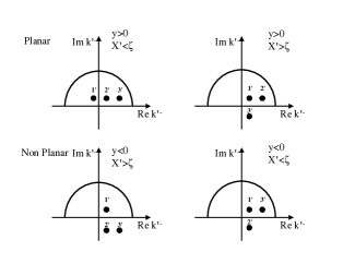
Figure 3: Representation of poles in the integration variable, $k^{-}$, complex plane for the multiparton diagrams of Fig.2.

We finally notice that the complications arising within partonic descriptions in the ERBL region were also addressed using Light Front Quark Models (LFQM) CRJi_01 ; CRJi_06 ; BroHwa ; BroDieHwa ; Miller ; Salme . In LFQM the contribution to the ERBL region is identified with “non-valence” type diagrams, which are also related to multiparton configurations, or higher Fock components in the hadronic wave function, and semi-disconnected diagrams do not appear. These are instead reinterpreted as an analytic continuation of the Bethe-Salpeter (BS) wave function, thus suggesting a simpler vacuum structure. However, a fully consistent connection with QCD would require that both an explicit treatment of hard rescattering contributions in the amplitude Braun , and, most importantly, of the analyticity properties are addressed. In this paper we showed that in order to establish the correct support, crossing symmetry, and analyticity properties that are necessary to establish dispersion relations, hence a partonic interpretation of GPDs, one needs a description beyond the identification of the proton off-forward structure functions with partonic wave functions. This can be accomplished by bringing into play FSI.

We thank R.L. Jaffe for helpful discussions.

References

- (1) X. D. Ji, Phys. Rev. D 55, 7114 (1997).
- (2) G.R. Goldstein and S. Liuti, Phys. Rev. D80, 071501 (2009).
- (3) S. Ahmad, H. Honkanen, S. Liuti and S. K. Taneja, Phys. Rev. D 75, 094003 (2007); ibid EPJC (2009).
- (4) S. J. Brodsky and F. J. Llanes-Estrada, Eur. Phys. J. C 46, 751 (2006).
- (5) A. Metz, S. Meissner and M. Schlegel, Mod. Phys. Lett. A 24, 2973 (2009).
- (6) R.L. Jaffe, Nucl. Phys. B229, 205 (1983); ibid Phys. Lett. 116B, 437 (1982).
- (7) M. Diehl and T. Gousset, Phys. Lett. B 428, 359 (1998)
- (8) M. Diehl, Phys. Rept. 388, 41 (2003).
- (9) G.R. Goldstein and S. Liuti, in preparation.
- (10) K. J. Golec-Biernat and A. D. Martin, Phys. Rev. D 59, 014029 (1998)
- (11) S. J. Brodsky, P. Hoyer, N. Marchals, S. Peigne and F. Sannino, Phys. Rev. D 65, 114025 (2002).
- (12) A.V. Belitsky, X. Ji and F. Yuan, Nucl. Phys. B 656, 165 (2003).
- (13) S. J. Brodsky, D. S. Hwang and I. Schmidt, Phys. Lett. B 530, 99 (2002).
- (14) C. R. Ji, Y. Mishchenko and A. Radyushkin, Phys. Rev. D 73, 114013 (2006)
- (15) L. S. Kisslinger, H. M. Choi and C. R. Ji, Phys. Rev. D 63, 113005 (2001)
- (16) B. C. Tiburzi and G. A. Miller, Phys. Rev. D 67, 054015 (2003); ibid B. C. Tiburzi and G. A. Miller, Phys. Rev. D 67, 054014 (2003).
- (17) S. J. Brodsky and D. S. Hwang, Nucl. Phys. B 543, 239 (1999)
- (18) S. J. Brodsky, M. Diehl and D. S. Hwang, Nucl. Phys. B 596, 99 (2001)
- (19) T. Frederico, E. Pace, B. Pasquini and G. Salme, Phys. Rev. D 80, 054021 (2009)
- (20) V. M. Braun, A. Lenz and M. Wittmann, Phys. Rev. D 73, 094019 (2006)