Coarsening to Chaos-Stabilized Fronts

Abstract

We investigate a model for pattern formation in the presence of Galilean symmetry proposed by Matthews and Cox [Phys. Rev. E 62, R1473 (2000)], which has the form of coupled generalized Burgers and Ginzburg-Landau-type equations. With only the system size $L$ as a parameter, we find distinct “small-$L$” and “large-$L$” regimes exhibiting clear differences in their dynamics and scaling behavior. The long-time statistically stationary state contains a single $L$-dependent front, stabilized globally by spatiotemporally chaotic dynamics localized away from the front. For sufficiently large domains, the transient dynamics include a state consisting of several viscous shock-like structures which coarsens gradually, before collapsing to a single front when one front absorbs the others.

In the exploration of the rich and diverse range of spatiotemporal dynamics observed in nonlinear, nonequilibrium spatially extended systems, it has proved particularly fruitful to investigate comparatively simple model partial differential equations (PDEs) whose solutions capture the essential features of the phenomena under investigation. Thus the Burgers equation has been extensively studied for the evolution and statistics of shocks; the Ginzburg-Landau (GL) equation and its generalizations describe the dynamics and stability of modulations of patterned states, while the Kuramoto-Sivashinsky and other models display spatiotemporal chaos (STC) Cross and Hohenberg (1993). In this paper we discuss a system describing the amplitude evolution for pattern formation with symmetry, which appears to combine features of several of these canonical systems and displays a surprising wealth of behaviors.

We investigate the Matthews-Cox (MC) equations Matthews and Cox (2000)

$$A_{T} = A+4A_{XX}-ifA,$$ (1)

$$f_{T} = f_{XX}-|A|^{2}_{X}$$ (2)

on a one-dimensional $L$-periodic domain, where $A$ is complex, $f$ is real, and $f_{X}\equiv\partial_{X}f\equiv\partial f/\partial X$ (similarly for the other derivatives). Equations (1)–(2) were initially derived in the context of the Nikolaevskiy PDE

$$u_{t}+uu_{x}=-\partial_{x}^{2}\left[\varepsilon^{2}-\left(1+\partial_{x}^{2}\right)^{2}\right]u.$$ (3)

This equation, proposed originally to model seismic wave behavior in viscoelastic media Beresnev and Nikolaevskiy (1993), and subsequently obtained in other contexts Tanaka (2004); Cox and Matthews (2007), appears to be a canonical model for short-wave pattern formation with reflection and Galilean symmetries. Unlike in more common pattern-forming contexts described at onset by the GL equation, the ${\mathcal{O}}(\varepsilon)$ stationary rolls in (3) are all unstable for all $\varepsilon>0$ Tribelsky and Velarde (1996); Tribelsky and Tsuboi (1996); Matthews and Cox (2000); Cox and Matthews (2007). Instead, solutions of (3) exhibit spatiotemporal chaos with strong scale separation Tanaka (2005); Wittenberg and Poon (2009), with coupling between the weakly unstable pattern at wave numbers $k\approx 1$ and the neutrally stable long-wave mode with $k\approx 0$. This suggests the Ansatz $u(x,t)\sim\varepsilon^{\alpha_{1}}A(X,T)e^{ix}+\text{c.c.}+\varepsilon^{\beta}f(X,T)+\dots$ for the envelopes $A$ and $f$ of the pattern and long-wave modes, respectively, where $X=\varepsilon x$, $T=\varepsilon^{2}t$. Matthews and Cox Matthews and Cox (2000) showed that the asymptotically self-consistent scaling as $\varepsilon\to 0$ is $\alpha_{1}=3/2$, $\beta=2$, and hence derived (1)–(2) from the Nikolaevskiy PDE as the leading-order modulation equations. While the scaling behavior on the attractor of (3) may be insufficiently described by this Ansatz Wittenberg and Poon (2009), the MC equations deserve study in their own right as generic amplitude equations for pattern formation with these symmetries Matthews and Cox (2000). Since (2) preserves the spatial mean of $f$, by Galilean invariance we may assume $f$ to have mean zero.

Chaos-stabilized fronts:

In describing properties of the MC equations (1)–(2), we emphasize the dynamics of the large-scale mode $f$, since the pattern amplitude $A$ appears to be driven by $f$. We note that several aspects of the behavior for relatively small $L$ have been previously described by Sakaguchi and Tanaka Sakaguchi and Tanaka (2007).

The snapshot of a solution for domain size $L=51.2\pi$ shown in Fig. 1

Figure 1: Snapshot at a fixed time $T_{1}=28000$ of $f(X,T_{1})$ (thick blue line) and $|A(X,T_{1})|$ (thin black line) for a solution of (1)–(2) with $L=51.2\pi\approx 160.8$.

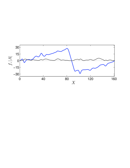
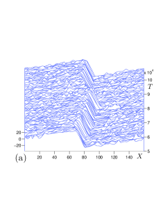
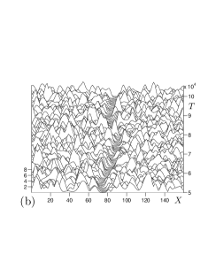
is typical of the statistically stationary behavior for “small” domains. The overall structure of $f$ resembles a perturbed viscous shock, with $f$ decreasing essentially linearly within the “front” region. Simultaneously, $|A|$ vanishes in the center of the front; Sakaguchi and Tanaka hence call this an “amplitude death” state Sakaguchi and Tanaka (2007). The time evolution of a typical solution shown in Fig. 2 clearly shows the invariance of the front structure in $f$ and the suppression of the roll amplitude $A$ within the front region.

Figure 2: Space-time plots of long-time solutions (a) $f(X,T)$ and (b) $|A(X,T)|$ of the MC equations for $L=51.2\pi$.

On the remainder of the domain, chaotic fluctuations in $f$ (on ${\mathcal{O}}(1)$ time scales) are superimposed on the approximately linear average positive slope, and correlated (in space and time) with chaos in $A$. This coexistence of an ordered front (amplitude death state) and a spatially localized spatiotemporally chaotic region is robust on all domains $L\gtrsim L_{0}$ large enough to sustain the front Sakaguchi and Tanaka (2007).

The space-time plot indicates that the overall viscous shock profile in $f$ is nonstationary, but maintains its shape up to small fluctuations; that is, short-time averages $\langle f(X,\cdot)\rangle_{\tau}$ are invariant up to translation. Denoting the averaged profile by $g(X)=g^{(L)}(X)$, where we center the front so $g(L/2)=0$, $g_{X}(L/2)<0$, and defining the front displacement $s(T)$ so that the instantaneous front position is $X_{s}(T)=L/2+s(T)$, we may decompose the large-scale mode as $f(X,T)=g(X-s(T))+\tilde{f}(X-s(T),T)$, where $\tilde{f}$ denotes fluctuations about the mean profile. The unsteady dynamics in $A$ and $\tilde{f}$ are then essentially confined to the region where $g_{X}\geq 0$ and to the vicinity of the local extrema of $g$ (see Fig. 3(c) below).

To help clarify this unusual behavior, we observe that the equation (2) for the large-scale mode $f$ has the form of a conservation law Sakaguchi and Tanaka (2007),

$$f_{T}=-J_{X}\,,\quad\text{where}\quad J=-f_{X}+|A|^{2}.$$ (4)

Taking long-time averages, $\langle J\rangle_{X}=-\langle f_{T}\rangle=0$, so in statistical equilibrium, the time-averaged flux $J$ is uniform in $X$, $\langle J\rangle=\langle-f_{X}+|A|^{2}\rangle\equiv\gamma$. Integrating over the domain and using periodicity, we find

$$\gamma=\gamma(L)=\frac{1}{L}\int_{0}^{L}\langle|A(X,\cdot)|^{2}\rangle\,dX>\ 0.$$ (5)

Now for a stationary amplitude death domain, where $\langle|A|^{2}\rangle=0$, we have $\gamma=-\langle f_{X}\rangle$; this confirms that amplitude death can occur only where $f$ is decreasing on average. (In fact, due to the apparent separation of time scales between the rapid fluctuations $\tilde{f}$ (on ${\mathcal{O}}(1)$ times) and the slow overall drift of the mean profile $g(X)$, short-time averaging seems sufficient to conclude $\langle f_{T}\rangle_{\tau}\approx 0$, so that the mean mid-front slope is $g_{X}(L/2)=-\gamma$.) By (5) the (averaged) slope $-\gamma$ of the large-scale mode $f$ in the center of the amplitude death state thus seems to be globally determined, being balanced by the mean-square amplitude of the pattern mode $A$ due to chaotic dynamics concentrated outside the front region.

Note that also $\gamma=\langle|A|^{2}\rangle$ wherever $\langle f_{X}\rangle=0$, relating the front slope to the fluctuations in $A$ at extrema of the averaged profile. Indeed, in the absence of $A$, $f$ satisfies a heat equation, and thus by (4) flows away from local maxima and towards local minima, destabilizing the front; the added forcing term in (2) when $|A|^{2}_{X}\not=0$ increases the flux $J$ so as to maintain the averaged overall flux balance, thereby stabilizing the (averaged) local extrema. The stabilization mechanism in the MC equations thus appears to act globally , with the chaotic dynamics being essential to sustaining the front (and amplitude death state); we denote the observed structures “chaos-stabilized fronts”.

(We remark that (1) does not contain the usual stabilizing GL cubic term, permitting (1)–(2) to support a family of exponentially growing solutions $A(X,T)=A_{0}e^{T}$, $f(X,T)=0$; that is, the MC equations do not have a bounded global attractor. However, these growing solutions are dynamically unstable, in the sense that they are overtaken by faster-growing spatially varying perturbations Matthews and Cox (2000); and in our numerical simulations we have not observed such solutions.)

To investigate the behavior of the MC equations on spatially periodic domains systematically, we have numerically integrated (1)–(2) using a pseudospectral method in space and an exponential time differencing (ETDRK4) scheme with step size $H=0.02$. The domain length $L$, the only free parameter in the system, was chosen to be $L=2\pi\times 64m/10$ for integers $m$ ranging from 2 to 64; correspondingly, we used between $2^{9}$ and $2^{14}$ Fourier modes. In computing time averages, we integrated until the system reached a statistically stationary single-front state, and then averaged over $10^{3}$-$10^{4}$ snapshots separated typically by time intervals $\Delta T=10$. All averaging was done within the frame of reference of the front; that is, we first determined the front displacement $s(T)$ and used it to align $A$ and $f$ so that the front was centered at $X=L/2$. In particular, the mean profiles were computed by $g(X)=\langle f(X+s(\cdot),\cdot)\rangle$.

Averaged profiles:

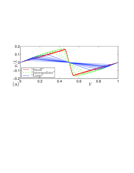
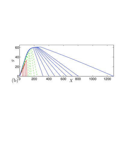
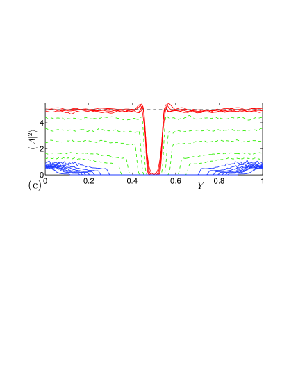
As seen in Fig. 3, the averages of $f$ and $|A|$ are, respectively, odd and even about $X=L/2$, recovering the reflection symmetry of the underlying PDEs (1)–(2). More interestingly, though, the time-averaged profiles $g(X)$ for $L\gtrsim L_{0}$ depend strongly on $L$, with the behavior falling into three distinct regimes:

Figure 3: (a), (b) Two representations of the long-time-averaged (centered) profile $g(X)=\langle f(X+s(\cdot),\cdot)\rangle$ of the large-scale mode $f$ for various $L$: (a) scaled horizontally and vertically, $L^{-1}g(LY)$ for $Y=X/L\in[0,1]$; (b) unscaled, half of the (odd) profile, $g(X)$ for $X\in[0,L/2]$. (c) Centered time-averaged pattern amplitude $\langle|A(LY,\cdot)|^{2}\rangle$. Domain sizes are (“small”: red) $L={25.6\pi}$, ${38.4\pi}$, ${51.2\pi}$, ${64\pi}$; (“intermediate”: green, dashed lines) $L={76.8\pi}$, ${89.6\pi}$, ${102.4\pi}$, ${128\pi}$, ${153.6\pi}$; and (“large”: blue) $L={204.8\pi}$, ${256\pi}$, ${307.2\pi}$, ${358.4\pi}$, ${409.6\pi}$, ${460.8\pi}$, ${512\pi}$ and ${819.2\pi}$. Averages were taken over time periods $T=1\times 10^{5}$ (small, intermediate) and $2\times 10^{4}$ (large), with $\Delta T=10$ between snapshots.

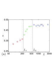
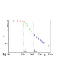
For relatively “small” domains, $L_{0}\lesssim L\lesssim L_{1}\approx 220$, the scaled profiles in Fig. 3(a) approximately coincide, indicating a scaling form for $g$: for some fundamental shape function $G$, periodic on $[0,1]$, we have $g(X)\approx LG(Y)$ (with $Y=X/L$). In this “small-$L$” regime the scaling relation is highly accurate within the front (but is weakly violated outside it: the slope $\alpha=g_{X}(0)$ in the active region increases slowly with $L$; see Fig. 4(a)); in particular, the midpoint slope is independent of $L$, with $-\gamma=g_{X}(L/2)=G^{\prime}(0.5)\approx-4.6$ (cf. Sakaguchi and Tanaka (2007)); see Fig. 4(b), where we have also numerically verified (5).

Figure 4: (a) Slope $\alpha=g_{X}(0)$ of averaged profile at midpoint of chaotic region. (b) Absolute value of mid-front slope $\gamma=-g_{X}(L/2)$ $(\Box)$, shown with the mean-square average pattern amplitude $L^{-1}\int_{0}^{L}\langle|A(X,\cdot)|^{2}\rangle\,dX$ $(\Diamond)$, verifying (5). Lengths $L$ and colors are as in Fig. 3; the vertical lines at $L_{1}\approx 220$ and $L_{2}\approx 560$ indicate approximate transitions between “small”, “intermediate” and “large” regimes.

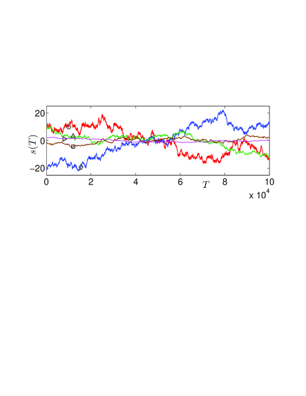
We also find that the relative sizes of the front and chaotic regions remain fixed, with $\langle|A|^{2}\rangle(X)\approx 5$ approximately constant and $L$-independent in the chaotic region (Fig. 3(c)). For these “small” domain sizes, the front translates over long times (recall Fig. 2); interestingly, the statistics of the front motion appear consistent with a random walk Poon (2009), as suggested by the trajectories of $s(T)$ shown in Fig. 5.

Figure 5: Representative trajectories of the front displacement $s(T)$ about $X=L/2$ for the “small” domains $L=38.4\pi\;(\circ)$ and $51.2\pi\;(\Diamond)$, and “intermediate” sizes $L=76.8\pi\;(\vartriangle)$, ${102.4\pi}\;(\Box)$, and ${153.6\pi}\;(\vartriangleright)$.

The (approximate) scaling form for the time-averaged profile $g(X)$ observed for “small” domains breaks down for larger $L$. Instead, for domain sizes in an “intermediate” regime with lengths $L_{1}\lesssim L\lesssim L_{2}\approx 560$, the amplitude of $g$ begins to level off, the front becomes wider and less steep, and chaotic fluctuations of $A$ and $f$ decrease in amplitude (see Figs. 3–4). Furthermore, the variance of the front displacement $s(T)$ decreases strongly with $L$, until the translation becomes imperceptible (Fig. 5).

This behavior is transitional to that of “large” domains $L\gtrsim L_{2}\approx 560$. In this regime the front is stationary, $s(T)\equiv 0$; the amplitude of $g(X)$ saturates at $\max g\approx 62$, as does the maximum slope in the chaotic region, $\alpha=g_{X}(0)\approx 0.5$. Indeed, Fig. 3(b) shows that the mean profile $g(X)$ near $X=0$ becomes invariant with increasing $L$; this saturation of the profile indicates to us that we have reached the large-$L$ asymptotic regime of (1)–(2). Since the width of the amplitude death region continues to grow with $L$, while the height is bounded, the front slope $-\gamma$ decays with $L$, and hence so does the amplitude of the fluctuations in $A$: for large $L$ the spatially localized chaotic dynamics superimposed on the mean profile are strongly suppressed.

Transient behavior:

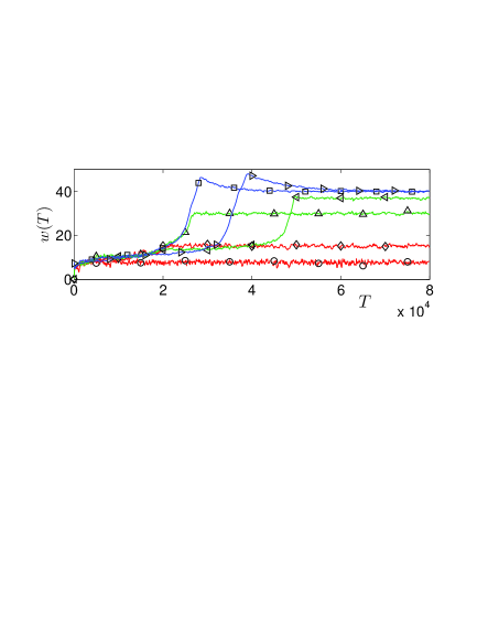
The strong $L$-dependence of the properties of the MC equations, within identifiable domain size regimes, is apparent also in the transient approach to the long-time statistically stationary state, as summarized in the time evolution of $w(T)=[L^{-1}\int_{0}^{L}f(X,T)^{2}\,dX]^{1/2}$ — analogous to an interface width in the context of surface growth — as in Fig. 6.

Figure 6: Evolution of $w(T)=[L^{-1}\int_{0}^{L}f(X,T)^{2}\,dX]^{1/2}$ for the “small” domains $L={25.6\pi\;(\circ)}$ and ${51.2\pi\;(\Diamond)}$, “intermediate” domains $L={89.6\pi\;(\vartriangle)}$ and ${128\pi\;(\vartriangleleft)}$; and “large” domains $L={256\pi\;(\Box)}$ and ${307.2\pi\;(\vartriangleright)}$, computed to $T=8\times 10^{4}$.

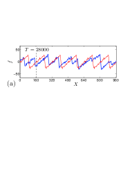
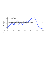
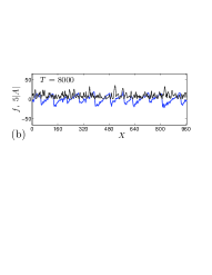
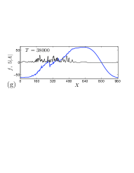
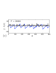
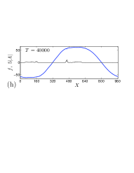
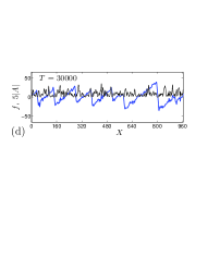
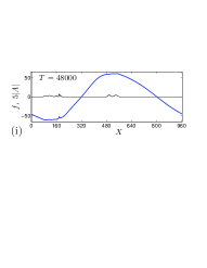
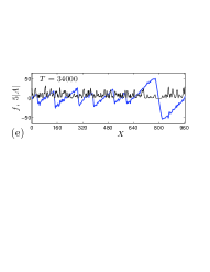
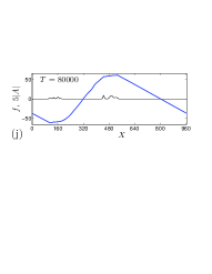
The snapshots from a typical time evolution for a “large” domain in Fig. 7

Figure 7: (a) Large scale mode $f$ at $T=28000$ for the “large” domain $L=307.2\pi$ with, for comparison, six copies of the $L=51.2\pi$ profile from Fig. 1. (b)–(j) Snapshots of $f$ and $|A|$ (for clarity we plot $5|A|$) showing coarsening and collapse to a single front for $L=307.2\pi\approx 964.8$.

demonstrate an extended coarsening period followed by a remarkable collapse to a single front:

From small random data, initial growth rapidly establishes a sawtooth pattern in $f$: a concatenation of structures, of varying widths and corresponding heights, locally reminiscent of the statistically stationary states in “small” domains (see Fig. 7(a)). Once this metastable state of multiple Burgers-like viscous shocks with superimposed chaotic fluctuations is established, a slow coarsening process ensues: front structures grow and merge with adjacent fronts, leading to a gradual increase of length scales and of $w(T)$ (Fig. 7(b)–(d)).

For “small” domains, for which the long-time state has the (approximate) scaling form $G$ on average, this coarsening concludes once there is a single front. However, for “intermediate” and “large” domains, the gradual growth of $w(T)$ through coarsening is followed by a “jump” in $w(T)$ (see Fig. 6) Poon (2009), reflecting qualitative changes in the profile $f(X,T)$, as seen in Fig. 7(d)–(h). Specifically, having (presumably) exceeded a critical size, one of the front structures begins to dominate, and then grows relatively rapidly by engulfing its neighbors until a state with an $L$-dependent single front is attained.

Finally, for “large” domains, $w(T)$ overshoots its asymptotic value (Fig. 6), since following the collapse to a single front, $f$ is initially nonlinear in the amplitude death region, before undergoing slow diffusive relaxation (by (2) with $|A|=0$) to the time-asymptotic linear front profile (Fig. 7(h)–(j)).

Discussion:

The structure of the Matthews-Cox equations (1)–(2) is reminiscent of that of other well-known systems. For instance, viewing (2) as a heat equation for $f$ with (localized chaotic) forcing, using the heat kernel to express $f$ as a quadratic functional of $A$ and substituting, the $-ifA$ coupling term in (1) acts as a nonlocal cubic stabilizing term in a GL-type equation. Alternatively, in the light of the viscous shock-like behavior in $f$, it may be fruitful to view (2) as a generalized viscous Burgers equation, with a nonlocal forcing term determined by (1). Such considerations may facilitate a theoretical understanding of the unusual behavior we have described in the MC equations.

We thank the IRMACS Centre at Simon Fraser University for providing a productive research environment, and David Muraki and Richard Kollár for helpful discussions. This work was partially supported by NSERC.

References

- Cross and Hohenberg (1993) M. Cross and P. Hohenberg, Rev. Mod. Phys. 65, 851 (1993).
- Matthews and Cox (2000) P. C. Matthews and S. M. Cox, Phys. Rev. E 62, R1473 (2000).
- Beresnev and Nikolaevskiy (1993) I. A. Beresnev and V. N. Nikolaevskiy, Physica D 66, 1 (1993).
- Tanaka (2004) D. Tanaka, Phys. Rev. E 70, 015202(R) (2004).
- Cox and Matthews (2007) S. M. Cox and P. C. Matthews, Phys. Rev. E 76, 056202 (2007).
- Tribelsky and Velarde (1996) M. I. Tribelsky and M. G. Velarde, Phys. Rev. E 54, 4973 (1996).
- Tribelsky and Tsuboi (1996) M. I. Tribelsky and K. Tsuboi, Phys. Rev. Lett. 76, 1631 (1996).
- Tanaka (2005) D. Tanaka, Phys. Rev. E 71, 025203(R) (2005).
- Wittenberg and Poon (2009) R. W. Wittenberg and K.-F. Poon, Phys. Rev. E 79, 056225 (2009).
- Sakaguchi and Tanaka (2007) H. Sakaguchi and D. Tanaka, Phys. Rev. E 76, 025201(R) (2007).
- Poon (2009) K.-F. Poon, Ph.D. thesis, Simon Fraser University (2009).