Calibrating spectral estimation for the LISA Technology Package with multichannel synthetic noise generation

Abstract

The scientific objectives of the Lisa Technology Package (LTP) experiment on board of the LISA Pathfinder mission demand for accurate calibration and validation of the data analysis tools in advance of the mission launch. The level of confidence required in the mission outcomes can be reached only by intensive testing the tools on synthetically generated data. A flexible procedure allowing the generation of cross-correlated stationary noise time series was set-up. Multichannel time series with the desired cross-correlation behavior can be generated once a model for a multichannel cross-spectral matrix is provided. The core of the procedure comprises a noise coloring, multichannel filter designed via a frequency-by-frequency eigen-decomposition of the model cross-spectral matrix and a subsequent fit in the Z-domain. The common problem of initial transients in filtered time series is solved with a proper initialization of the filter recursion equations. The noise generator performance was tested in a two-dimensional case study of the closed-loop LTP dynamics along the two principal degrees-of-freedom.

Introduction

The LTP (LISA Technology Package) experiment is the main scientific payload on the European Space Agency mission, LISA Pathfinder. Its goal is to determine and analyse all possible sources of disturbance which perturb the free-falling test masses from their geodesic motion. The system is composed of two test masses whose position is sensed by an interferometer. The spacecraft cannot simultaneously follow both masses, and so the trajectory of only one test mass serves as the drag-free reference along the $x$ (measurement) axis. To prevent the trajectories of the two masses from diverging in response to any differential force, the second test mass is electrostatically actuated to follow the spacecraft. In the main science operating mode, the position of the SC relative to the first test mass is controlled using micro-Newton thrusters attached to the SC. The position of the second test mass is controlled using capacitive actuators surrounding the test mass. The first interferometer channel measures the position of the first test mass relative to the spacecraft. The second interferometer channel (differential channel) measures the relative displacement between the two test masses.

A set of different experiments, such as measurements of parasitic voltages, test mass charging, thermal and magnetic disturbances, completely covers the scheduled 90 days of LTP operations; the overall aim of the experiments is to reach the best free-fall quality in a step by step procedure in which the result of the previous experiment is used to define the detailed configuration of the following experiment. This cascade-like process aims to demonstrate the ability to put a test mass into free-fall at a level where any residual acceleration is below $3\times 10^{-14}\textnormal{ m}\textnormal{ s}^{-2}/\sqrt{\textnormal{Hz}}$ at frequencies around $1$ mHz Armano ; Anza ; McNamara ; Bortoluzzi1 ; Bortoluzzi2 .

Such a demanding accuracy requires a careful calibration of the spectral estimation algorithms so as to avoid any systematic bias in the estimation of the spectrum of the residual acceleration. Due to the limited time duration of the mission, the amount of data available will be not enough for a meaningful and robust calibration of the dedicated data analysis tools. The natural way to solve the problem is to calibrate and test the tools in advance of the mission, by an in-depth analysis of synthetic noise data. The experiment has a total of $18$ measuring channels sensing the movement of the test masses, many of which are coupled so that information is contained not only in the individual power-spectra, but also in the cross spectral densities between different channels. In order to set-up a reliable test bench for such a system, a robust and flexible multichannel noise generator is required.

The problem of generating a sequence of random variables having some definite statistical properties is well examined in literature. Stein and Storer stein proposed a procedure for which the computation of $N$ sample values requires the eigen-decomposition of the covariance matrix of the process. This allows the identification of a transformation matrix that multiplies a vector of independent samples to provide a noise series with the desired correlation properties. Levin Levin suggested instead to pass white noise through a digital noise coloring filter with a rational transfer function. The problem connected with the initial transient is solved with the calculation of $K$ consecutive ($K$ is the order of the noise shaping filter) output values having the same statistical properties as if they were produced by steady-state operation of the filter. An alternative method for filter initialization was indicated by Kay Kaypaper who realized that one has just to specify the initial state for the filter. The method for the calculation of the initial state is based on the Levinson-Durbin algorithm. As an alternative, Franklin Franklin described a procedure for the simulation of stationary and non-stationary Gaussian random processes. The procedure for a non-stationary process is similar to that reported in stein and is based on the Crout factorization of the covariance matrix of the process. The output for the stationary case is, instead, the result of a simulation of a continuous system by means of the state space formalism. The initial state is calculated with a linear transformation from uncorrelated random noise samples. All the methods in literature deal with the generation of a single channel of data with a given correlation function or, analogously, with a given spectrum. The algorithms proposed by Levin, Kay and Franklin can be crudely summarized in three steps; 1) identification of the desired system, 2) initialization of the data sequence, 3) generation of the colored noise data sequence from a sequence of zero mean, delta correlated random numbers.

The method proposed in the present paper follows this classical scheme with the relevant difference that it is designed to work with multichannel systems (i.e. multiple inputs, multiple outputs). In the following, the mathematical basis of the method is developed, and a case study is discussed in order to quantitatively assess the reliability of the procedure.

I Principles of the noise generation procedure

It can be assumed, in complete generality, that the noise to be generated $x\left(t\right)$ has a power spectral density (PSD) that can be written as:

$$S_{xx}\left(\omega\right)=\left|H\left(\omega\right)\right|^{2}S_{0}.$$ (1)

The process $x\left(t\right)$ can be thought as the output of a rational continuous filter with transfer function $H\left(\omega\right)$, at the input of which is a white, zero-mean noise $\epsilon\left(t\right)$ with PSD equal to $S_{0}$. The filter $H\left(\omega\right)$ can be written as:

$$H\left(\omega\right)=\sum_{h=1}^{N}{\frac{r_{h}}{\imath\omega-p_{h}}},$$ (2)

with $r_{h}$ the residue of $H\left(\omega\right)$ in $p_{h}$ .

Equation (2) shows that the process $x\left(t\right)$ can in turn be considered as:

$$x\left(t\right)=\sum_{h=1}^{N}{y_{h}\left(t\right)},$$ (3)

where:

$$y_{h}\left(t\right)=r_{h}\int\limits_{0}^{\infty}e^{p_{h}t^{\prime}}\epsilon\left(t-t^{\prime}\right)\,dt^{\prime}.$$ (4)

Thus, generating the process $x\left(t\right)$ is equivalent to generating the $N$ correlated processes $y_{h}\left(t\right)$. A discrete process with time-step $T$ can be realized from the recursive equations:

$$y_{h}\left(t+T\right) = y_{h}\left(t\right)e^{p_{h}T}+\epsilon_{h}\left(t+T\right)$$

$$\epsilon_{h}\left(t+T\right) = r_{h}\int\limits_{0}^{T}e^{p_{h}t^{\prime}}\epsilon\left(t+T-t^{\prime}\right)\,dt^{\prime}$$

$$h = 1,\ldots,N.$$ (5)

Since the procedure must not diverge, only poles $p_{h}$ with a negative real part (stable poles) are considered. The processes $\epsilon_{h}\left(t+T\right)$ are not independent but it can be verified that their cross-correlations is vanishing for time intervals larger than $T$. Then, indicating with $k$ and $m$ integers values, the cross-correlation between input processes can be written as:

$$\langle\epsilon_{i}\left(kT\right)\epsilon_{j}\left(mT\right)\rangle=\delta_{km}\frac{S_{0}r_{i}r_{j}}{p_{i}+p_{j}}\left[e^{\left(p_{i}+p_{j}\right)T}-1\right],$$ (6)

where the notation $\left\langle\right\rangle$ indicates the expectation value operator. If the process $\epsilon\left(t\right)$ is zero-mean Gaussian, then so is $\epsilon_{j}\left(kT\right)$, and equation (6) is sufficient to determine the statistics.

The generated series $x\left(kT\right)$ exactly represents the sampling of the continuous process $x\left(t\right)$ with a time-step $T$, and therefore it also reproduces the aliasing if the filter $H\left(\omega\right)$ has a response different from zero at frequencies larger than $1/2T$. This is a consequence of the well known relation between the spectra of discrete and continuous processes Percival :

$$\bar{S}_{xx}\left(\omega\right) = \sum_{k=-\infty}^{\infty}S_{xx}\left(\omega+\frac{2\pi k}{T}\right)$$

$$\left|\omega\right| \leq \frac{2\pi k}{T}.$$ (7)

Here $T$ is the sampling time, $\bar{S}_{xx}\left(\omega\right)$ and $S_{xx}\left(\omega\right)$ are the spectra of the discrete and continuous processes respectively.

From the point of view of the numerical implementation, it is more convenient to start from the assumption of a discrete filter. In the case of finite length discrete time series, equations (1) and (2) can be rewritten as:

$$S_{xx}\left(\Omega\right) = \left|H\left(\Omega\right)\right|^{2}S_{0}.$$

$$H\left(\Omega\right) = \sum_{h=1}^{N}{\frac{r_{h}}{1-p_{h}e^{-\imath\Omega}}},$$ (8)

where $\Omega$ is the normalized angular frequency $\Omega=2\pi f/f_{s}$, and $f_{s}$ is the sampling frequency.

Each element of the partial-fraction expansion in equation (8) can be considered as a simple autoregressive moving average filter for which the usual recursive relation holds papoulis :

$$x\left(n\right) + a_{1}x\left(n-1\right)+\cdots+a_{N}x\left(n-N\right)=b_{0}i\left(n\right)+\cdots+b_{M}i\left(n-M\right)$$

$$a_{1} = -p\text{ and }a_{2},\ldots,a_{N}=0$$

$$b_{0} = r\text{ and }b_{1},\ldots,b_{M}=0.$$ (9)

Here, $a_{i}$ are the coefficients of the denominator polynomial, $b_{j}$ are the coefficients of the numerator polynomial, $r$ and $p$ are residues and poles as written in equation (8) and $i\left(n-k\right)$ is the step $k$ delayed input to the system. Thus the complete noise generation process is obtained by:

$$x\left(n\right) = \sum_{k=1}^{N}x_{k}\left(n\right)$$

$$x_{k}\left(n\right) = p_{k}x_{k}\left(n-1\right)+r_{k}\epsilon\left(n\right).$$ (10)

Each $x_{k}\left(n\right)$ can be generated according to the recursive equation (10) starting from the same white noise series $\epsilon\left(n\right)$.

Such a procedure provides a noise series whose PSD is an accurate replica of the continuous noise spectrum up to the Nyquist frequency. Aliasing is not reproduced in the discrete case. In the rest of the paper, the detailed calculations for the implementation of a discrete multichannel procedure are presented.

II Multichannel noise generation

II.1 Noise Coloring Filter Identification

A multichannel sequence can be described by the $M$-dimensional vector:

$$\mathbf{y}\left(t\right)=\left({\begin{array}[]{*{20}c}{y_{1}\left(t\right)}\\ \vdots\\ {y_{M}\left(t\right)}\\ \end{array}}\right),$$ (11)

where $y_{i}\left(t\right)$ is the data sequence at the ith channel. If the process is stationary, the cross-correlation matrix at a given delay $\tau$ is defined as kay :

$$\mathbf{R}\left(\tau\right)=\int\limits_{-\infty}^{\infty}{\mathbf{y}\left(t\right)\mathbf{y}^{\dagger}\left({t+\tau}\right)}\mathrm{d}t.$$ (12)

The elements of the matrix $\mathbf{R}\left(\tau\right)$ are the cross-correlations between the different elements of the multichannel sequence. The symbol $\dagger$ indicates a matrix conjugate transpose. The cross-spectral density matrix for the given multichannel process is defined as the Fourier transform of the cross-correlation matrix:

$$\mathbf{S}\left(\omega\right) = \int\limits_{-\infty}^{\infty}\mathbf{R}\left(\tau\right)\exp\left(-\imath\omega\tau\right)\mathrm{d}\tau$$

$$\mathbf{S}\left(\omega\right) = \left({\begin{array}[]{*{20}c}{S_{11}\left(\omega\right)}&\cdots&{S_{1M}\left(\omega\right)}\\ \vdots&\ddots&\vdots\\ {S_{M1}\left(\omega\right)}&\cdots&{S_{MM}\left(\omega\right)}\\ \end{array}}\right).$$ (16)

A noise coloring multichannel filter is a linear operation which transforms a delta correlated unitary variance multichannel random sequence (multichannel white noise $\bm{\varepsilon}\left(t\right)$) in to a noise sequence with the given cross-spectral density matrix.

$$y_{i}\left(t\right)=\sum\limits_{j=1}^{N}\int\limits_{-\infty}^{\infty}h_{ij}\left(\tau\right)\varepsilon_{j}\left(t-\tau\right)\mathrm{d}\tau$$

$$\left\langle\varepsilon_{i}\left(t\right)\varepsilon_{j}\left(t+\tau\right)\right\rangle=\delta_{ij}\delta\left(\tau\right),$$ (17)

where $h_{ij}\left(\tau\right)$ is the impulse response of the filter between the jth input and the ith output. Assuming that the number of input channels $N$ is the same as the number of output channels $M$, the multichannel coloring filter can be represented by a square matrix. The cross-spectral matrix of the output process can be obtained by the combination of the cross-spectral matrix of the input and the frequency response of the filter:

$$\mathbf{S}\left(\omega\right)=\mathbf{H}\left(\omega\right)\cdot\mathbf{I}\cdot\mathbf{H}^{\dagger}\left(\omega\right).$$ (18)

Here $\mathbf{I}$ is the unit matrix corresponding to the cross-spectral matrix of the input multichannel white noise process $\bm{\varepsilon}\left(t\right)$ and $\mathbf{H}\left(\omega\right)$ is the frequency response matrix of the multichannel filter. The problem of the generation of a multichannel noise series with the given cross-spectral matrix starts from the identification of the noise coloring filter $\mathbf{H}\left(\omega\right)$.

The eigendecomposition of the cross-spectral matrix $\mathbf{S}\left(\omega\right)$ is defined as:

$$\mathbf{S}\left(\omega\right)=\mathbf{V}\left(\omega\right)\cdot\bm{\Sigma}\left(\omega\right)\cdot\mathbf{V}^{-1}\left(\omega\right),$$ (19)

where $\mathbf{V}\left(\omega\right)$ and $\bm{\Sigma}\left(\omega\right)$ are the eigenvector and eigenvalue matrices of the cross-spectral matrix $\mathbf{S}\left(\omega\right)$. Since $\mathbf{S}\left(\omega\right)$ is Hermitian, its eigenvector matrix is unitary, i.e. $\mathbf{V}\left(\omega\right)\mathbf{V}^{\dagger}\left(\omega\right)=\mathbf{I}$. Therefore, combining equations (18) and (19), the noise coloring filter can be obtained:

$$\mathbf{H}\left(\omega\right)=\mathbf{V}\left(\omega\right)\cdot\sqrt{\bm{\Sigma}\left(\omega\right)}.$$ (20)

As $\bm{\Sigma}\left(\omega\right)$ is a diagonal matrix, $\sqrt{\bm{\Sigma}\left(\omega\right)}$ is a diagonal matrix with elements given by the square root of the elements of $\bm{\Sigma}\left(\omega\right)$.

II.2 System Discretization

Once the frequency response of the coloring filter $\mathbf{H}\left(\omega\right)$ is known, a discrete multichannel filter is required for the generation of discrete synthetic noise data series. Discrete filters can be estimated by a least square fit procedure carried out in the frequency domain. Such a process can produce a set of discrete autoregressive moving average (ARMA) filters which together reproduce the multichannel system frequency response to the given accuracy. The fitting process is based on a modified version of the vector fitting algorithm vectfit1 ; vectfit2 adapted to work in Z-domain vectfit3 . This procedure allows the frequency response of the coloring filter to be fit with ARMA functions expanded in partial fractions:

$$\mathbf{H}\left(\omega\right) = \left({\begin{array}[]{*{20}c}{h_{11}\left(\omega\right)}&\cdots&{h_{1M}\left(\omega\right)}\\ \vdots&\ddots&\vdots\\ {h_{M1}\left(\omega\right)}&\cdots&{h_{MM}\left(\omega\right)}\\ \end{array}}\right)\to\mathbf{H}\left(z\right)=\left({\begin{array}[]{*{20}c}{h_{11}\left(z\right)}&\cdots&{h_{1M}\left(z\right)}\\ \vdots&\ddots&\vdots\\ {h_{M1}\left(z\right)}&\cdots&{h_{MM}\left(z\right)}\\ \end{array}}\right)$$ (27)

$$h_{ij}\left(z\right) = \sum\limits_{k=1}^{N}{\frac{{r_{ij,k}}}{{1-p_{ij,k}z^{-1}}}}.$$ (28)

The number of poles required to obtain a satisfactory fit of the model transfer function is automatically determined by an iterative procedure in which the number of poles is increased by one at each step of the fit loop. The iteration stops when the mean square error between fit function response and model response comes to a value smaller than the user-defined threshold. Since the fit is performed in the Z-domain, the noise generation procedure turn out to be free from aliasing as discussed in section I.

It is worth noting that the eigenvectors in equation (19) are defined up to an arbitrary phase factor. This means that the columns of the $\mathbf{V}\left(\omega\right)$ matrix can be multiplied by an arbitrary phase factors $e^{i\phi}$ without changing their property of being eigenvectors of the cross-spectral matrix. Such phase arbitrariness does not extend to the single elements in the columns of $\mathbf{V}\left(\omega\right)$; they are elements of the same eigenvector of $\mathbf{V}\left(\omega\right)$ and their phase relation must be carefully preserved during the fit process because it is connected to the correlation properties of the multichannel system. It can happen, after the eigen-decomposition process, that the phase of the elements of $\mathbf{V}\left(\omega\right)$ is such that the frequency response of the elements of $\mathbf{H}\left(\omega\right)$ cannot be fit with stable poles. In that case, the poles must be stabilized after the fit process by the application of an all-pass filter papoulis . The all-pass function substitutes unstable poles with the inverse of their conjugates which are stable. Its magnitude (absolute value) is 1 at each frequency. As already mentioned, the phase relation between the elements of each column of $\mathbf{H}\left(z\right)$ must be kept constant to prevent the corruption of the system correlation properties. The proper all-pass filter for the elements of $\mathbf{H}\left(z\right)$ stabilizes the unstable poles of the given $h_{ij}\left(z\right)$ and at the same time adds an extra phase in order to keep the phase relation between the columns of $\mathbf{H}\left(z\right)$ constant. Therefore each element of $\mathbf{H}\left(z\right)$ is modified according to:

$$h_{\alpha\beta}\left(z\right) \to h_{\alpha\beta}\left(z\right)\prod\limits_{k=1}^{N_{\alpha\beta}^{u}}{\left({\frac{{z-p_{\alpha\beta,k}}}{{zp_{\alpha\beta,k}^{*}-1}}}\right)}\left\{\prod\limits_{\gamma\neq\alpha}\left[\prod\limits_{h=1}^{N_{\gamma\beta}^{u}}{\left({\frac{{z-p_{\gamma\beta,h}}}{{zp_{\gamma\beta,h}^{*}-1}}}\right)}\right]\right\}$$

$$\alpha,\beta,\gamma = 1,\cdots,M.$$ (29)

Here, $N_{\alpha\beta}^{u}$ is the number of unstable poles in $h_{\alpha\beta}\left(z\right)$. The function $\prod\limits_{k=1}^{N_{\alpha\beta}^{u}}{\left({\frac{{z-p_{\alpha\beta,k}}}{{zp_{\alpha\beta,k}^{*}-1}}}\right)}$ has the purpose of poles stabilization for the element $h_{\alpha\beta}\left(z\right)$ of $\mathbf{H}\left(z\right)$. The product $\prod\limits_{\gamma\neq\alpha}\left[\prod\limits_{h=1}^{N_{\gamma\beta}^{u}}{\left({\frac{{z-p_{\gamma\beta,h}}}{{zp_{\gamma\beta,h}^{*}-1}}}\right)}\right]$ provides an extra phase coming from the poles stabilization procedure for the other elements of the same column of $\mathbf{H}\left(z\right)$. In this way, each element of the matrix $\mathbf{H}\left(z\right)$ comes with such a phase allowing the representation with just stable poles and, at the same time, the original phase relation between elements of the same column of $\mathbf{H}\left(z\right)$ is preserved. A second fit step with stable poles provides usable filters for noise generation.

II.3 Filter Initialization

The output of a linear discrete causal filter is a function of the present and all previous input values. Since the input to the filter must start at some time $t=0$, the output process will consist of an unwanted filter transient response added to the desired stationary random process. One possible approach to handle the problem of the filter transients is to wait for the time necessary for the transients to decay to an acceptable level. However the transient response is proportional to the filter impulse response and if there are poles too near the unitary circle of the complex plane the transient response could last for an unacceptably long time. Moreover the practice of hand removing initial data is always inaccurate and can hide important features or introduce fake signals especially when the spectrum spans several decades in frequency. Therefore the filter for the noise generation should be always properly initialized.

We are searching for an initialization for the recursive equation of a ARMA process written as sum of partial fractions (Figure (1), Equation (28)):

$$x_{ij,k}\left(n\right) = p_{ij,k}x_{ij,k}\left({n-1}\right)+r_{ij,k}\varepsilon_{j}\left(n\right)$$

$$y_{ij}\left(n\right) = \sum\limits_{k=1}^{N_{ij}}{x_{ij,k}\left(n\right)}.$$ (30)

Figure 1: Scheme for the application of a multichannel filter expanded in partial fractions.

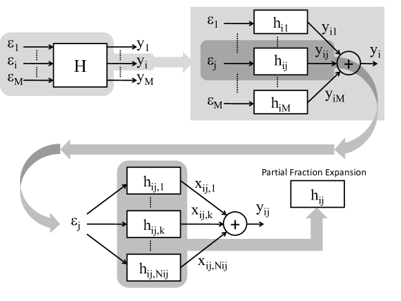
The recursive equation (30) calculates the output of the system at a given time on the basis of the input $\varepsilon_{j}\left(n\right)$ at the same time and the information from the previous output $x_{ij,k}\left({n-1}\right)$. In the present case the input process $\varepsilon_{j}\left(n\right)$ is an element of a discrete multichannel unitary variance white noise process such that:

$$\left\langle{\varepsilon_{i}\left(n\right)\varepsilon_{j}\left(m\right)}\right\rangle=\delta_{i,j}\delta_{n,m}.$$ (31)

In order to properly initialize the recursive equations for the implementation of the multichannel filter, it is necessary to calculate the covariance matrix of the initial states $x_{ij,k}\left(0\right)$. It should be considered that the $M^{2}$ processes represented in equation (17) are not independent from each other. A combined process should be defined in which all the recursive equations (equation 30) for each of the $M^{2}$ processes are incorporated. Readily it is seen that, thanks to the delta correlation properties (31) of the input signals, the processes applied to different input data series are independent. This means that, instead of building a single combined process, one has to build $M$ independent processes which combine those applied to the same input. The new processes can then be written as:

$$\bm{\chi}_{j}\left(n\right) \to \left\{\begin{array}[]{l}x_{1j,1}\left(n\right)=p_{1j,1}x_{1j,1}\left({n-1}\right)+r_{1j,1}\varepsilon_{j}\left(n\right)\\ \vdots\\ x_{1j,N_{1j}}\left(n\right)=p_{1j,N_{1j}}x_{1j,N_{1j}}\left({n-1}\right)+r_{1j,N_{1j}}\varepsilon_{j}\left(n\right)\\ \vdots\\ x_{Mj,1}\left(n\right)=p_{Mj,1}x_{Mj,1}\left({n-1}\right)+r_{Mj,1}\varepsilon_{j}\left(n\right)\\ \vdots\\ x_{Mj,N_{Mj}}\left(n\right)=p_{Mj,N_{Mj}}x_{Mj,N_{Mj}}\left({n-1}\right)+r_{Mj,N_{Mj}}\varepsilon_{j}\left(n\right)\\ \end{array}\right.$$ (39)

$$j = 1,\cdots,M.$$ (40)

The covariance of such processes (40) can be written as:

$$\left\langle{\chi_{i,\alpha}\left(n\right)\chi_{j,\beta}^{*}\left(m\right)}\right\rangle = \left\langle{p_{i,\alpha}\chi_{i,\alpha}\left({n-1}\right)p_{i,\alpha}^{*}\chi_{j,\beta}^{*}\left({m-1}\right)}\right\rangle+\left\langle{r_{i,\alpha}\varepsilon_{i}\left(n\right)r_{i,\beta}^{*}\varepsilon_{j}^{*}\left(m\right)}\right\rangle$$

$$\alpha = 1,\ldots,N_{1i}+\cdots+N_{Mi}$$

$$\beta = 1,\ldots,N_{1j}+\cdots+N_{Mj}$$

$$i,j = 1,\cdots,M.$$ (41)

Where again, the symbol $\left\langle\right\rangle$ represents the expectation value operator. Assuming stationary processes:

$$\left\langle{\chi_{i,\alpha}\left(n\right)\chi_{j,\beta}^{*}\left(m\right)}\right\rangle=R_{ij,\alpha\beta}\left({n,m}\right)=R_{ij,\alpha\beta}\left({n-m}\right),$$ (42)

and thanks to the properties of the input functions (31):

$$R_{ij,\alpha\beta}\left({n-m}\right)=\frac{{r_{i,\alpha}r_{j,\beta}^{*}}}{{1-p_{i,\alpha}p_{j,\beta}^{*}}}\delta_{ij}\delta\left({n-m}\right),$$ (43)

which provides the desired covariance for the first state of the recurrence sequences:

$$R_{j,\alpha\beta}\left(0\right)=\frac{{r_{j,\alpha}r_{j,\beta}^{*}}}{{1-p_{j,\alpha}p_{j,\beta}^{*}}}.$$ (44)

Initial states for the filter recurrence sequence can then be generated by a multivariate noise generator according to the given covariance (44). As an alternative, they can be calculated from random independent variables through a linear transformation stein of the type:

$$\bm{\chi}_{j}\left(0\right)=\mathbf{A}_{j}\cdot\bm{\eta}_{j},$$ (45)

where $\bm{\eta}_{j}$ is a column vector of $N_{1j}+\cdots+N_{Mj}$ independent zero mean and unit variance random numbers and ${\mathbf{A}}_{j}$ is a $\left({N_{1j}+\cdots+N_{Mj}}\right)\times\left({N_{1j}+\cdots+N_{Mj}}\right)$ transformation matrix. If $R_{j,\alpha\beta}\left(0\right)$ is calculated for the variables in equation (45), it is found:

$$\mathbf{R}_{j}\left(0\right) = \left({{\mathbf{A}}_{j}\cdot\bm{\eta}_{j}}\right)\cdot\left({{\mathbf{A}}_{j}\cdot\bm{\eta}_{j}}\right)^{\dagger}$$ (46)

$$= {\mathbf{A}}_{j}\cdot{\mathbf{I}}\cdot{\mathbf{A}}_{j}^{\dagger},$$

and it is readily seen that:

$${\mathbf{A}}_{j}=\mathbf{V}_{j}\cdot\sqrt{\bm{\Sigma}_{j}},$$ (47)

where $\mathbf{V}_{j}$ and $\bm{\Sigma}_{j}$ are the eigenvector and eigenvalue matrices of $\mathbf{R}_{j}\left(0\right)$.

III A case study, LTP along $X$ axis

III.1 Response model and fit

An application of the noise generation procedure is presented for a two channel system simulating the LISA Technology Package (LTP) along the principal measurement axis Armano ; Anza ; McNamara ; Bortoluzzi1 ; Bortoluzzi2 ; LISA7Anneke ; LISA7Martin ; LISA7Luigi . The complete set of algorithms are available as MATLAB tools in the framework of the LTPDA toolbox LISA7Martin ; matlab and can be freely downloaded, together with the complete toolbox, at the LTPDA project web page ltpda .

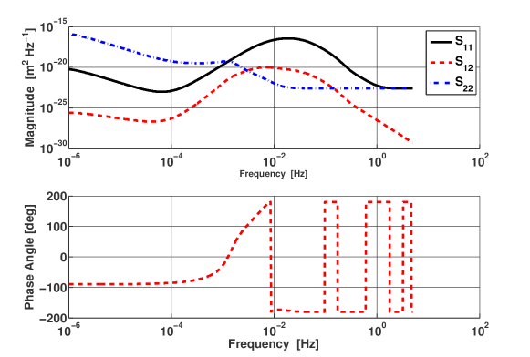
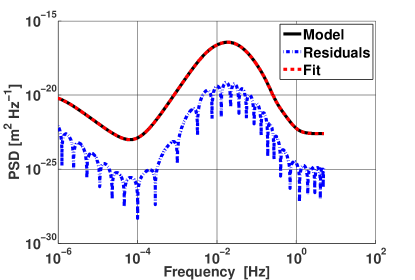
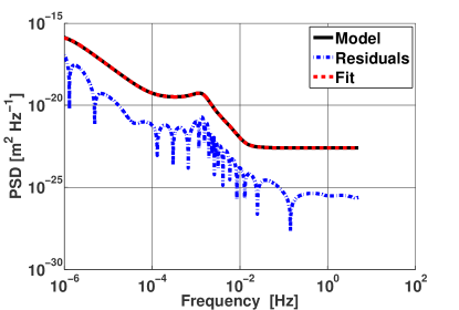
The expected power spectra and cross-power spectrum at the output of the system can be calculated (Figure (2)) on the basis of some assumptions on the properties of input noise sources Bortoluzzi1 . The noise coloring filters can be calculated following the procedure described in paragraphs II.1 and II.2. A frequency domain fit is performed on the models for the coloring filters obtained by eigendecomposition (frequency by frequency) of the expected cross-spectral density matrix. The fit procedure takes around $200$ seconds on a standard desktop machine . The four transfer functions $h_{11}\left(z\right)$, $h_{12}\left(z\right)$, $h_{21}\left(z\right)$ and $h_{22}\left(z\right)$ have respectively $25$, $30$, $28$ and $30$ poles. The fit loop stops when the mean square error between fit function response and model response is smaller than $1\times 10^{-4}$. The response of the filter designed to reproduce the cross-spectral density can be calculated according to equation (18). It can then be compared with the model cross-spectral density of the system as reported in figure 3.

Figure 2: Model power spectra and cross-spectrum for the signals at the output of the two channels. $S_{11}$ and $S_{22}$ are real values so they do not appear in the bottom plot.

(a)

(b)

Figure 3: Comparison between model power spectral densities and fit result. a) Output of the first channel. b) Output of the second channel.

In order to compare the correlation properties of expected model with the fit results, it is useful to introduce the complex cross-coherence:

$$\rho\left(\omega\right)=\frac{{S_{12}\left(\omega\right)}}{{\sqrt{S_{11}\left(\omega\right)S_{22}\left(\omega\right)}}},$$ (48)

where $S_{12}\left(\omega\right)$, $S_{11}\left(\omega\right)$ and $S_{22}\left(\omega\right)$ are cross-spectrum and power spectra of the first and second channels. The real and imaginary part of the cross-coherence for the expected and fit cross-spectral matrices are reported in figure 4.

(a)

(b)

Figure 4: Comparison between expected coherence and fit result. a) Real part. b) Imaginary part.

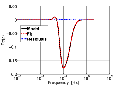
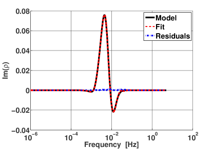
Any discrepancy between the expected model and the fit model can be considered as a systematic error in the procedure, whose influence on the process can be minimized by increasing the fit accuracy. Clearly this has a computational cost in terms of the number of poles required to match the accuracy goal and on the amount of time required to complete the fit loop. Hereafter, the fit model will be considered as the reference model.

III.2 Noise generation tests

Once the two channel noise coloring filter is obtained it can be used to generate a two channel noise data series according to the procedure described in paragraph II.3. Data series are $3\times 10^{5}$ seconds long at a sampling rate of $10$ Hz. The chosen rate is the same as the LTP experiment operations, e.g., the control forces acting on test masses and the spacecraft will be calculated by controllers on the basis of $10$ Hz sampled data streams.

In order to realize a statistically meaningful test, $N=500$ independent realizations of the two channel process were generated. Power spectra of the two channels are calculated with the windowed periodogram method using a 4-term Blackman-Harris window Harris . The choice of such a window is justified by the requirements in terms of spectral leakage performances. A 4-term Blackman-Harris window, having the highest side-lobe level of -$92$ dB (relative to the main lobe level) Harris , is indeed one of the best-performing available window in terms of spectral leakage suppression. The $N$ realizations of the power spectrum were averaged and compared with the reference model expectation (figure 5).

The reported uncertainty is calculated under the assumption that $\sigma_{mean}\left(\omega\right)=\frac{\sigma_{pop}\left(\omega\right)}{\sqrt{N}}$, where $\sigma_{pop}\left(\omega\right)$ is the sample standard deviation of the spectra population at a given frequency. In doing this we have considered that, since the power spectrum of a $\chi^{2}_{2}$ distributed variable Jenkins , the mean of $N$ independent realization of the same spectrum will also be $\chi^{2}_{2N}$ distributed. Since in our case $N=500$, the average of the spectra is $\chi^{2}$ distributed with $1000$ degrees of freedom, and such a variable can be considered to be Gaussian distributed with reasonable accuracy . The expected standard deviation (normalized to the mean) for the equivalent normal distribution is $0.045$ where we measure on average $\sigma_{mean}=0.044\pm 0.002$ .

Figure 5: Averaged power spectral density compared with reference model. a) First channel. b) Second channel.

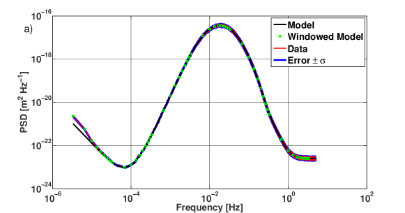
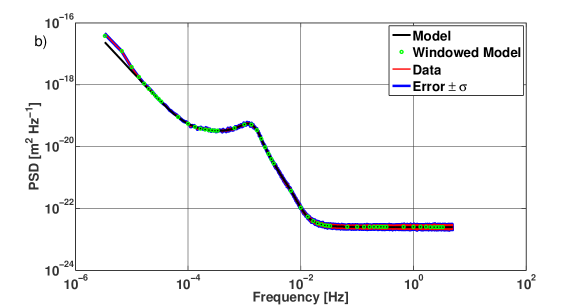
In the procedure for the calculation of the power spectrum, data are multiplied in the time domain for the time response of the window function. As this operation corresponds to a convolution in the frequency domain, the reference model must include also the effect of the window function. Windowed spectra can be calculated as:

$$S_{w}\left(\psi=\frac{2\pi k}{N}\right)=\frac{1}{2\pi N}\int\limits_{-\pi}^{\pi}S\left(\Omega\right)\left|\sum_{q=0}^{N-1}w_{q}e^{\imath q\left(\Omega-k\frac{2\pi}{N}\right)}\right|^{2}\,d\Omega,$$ (49)

where $N$ is the number of samples in the data series and $w_{q}$ are the time samples of the window function. The integral in equation (49) is numerically evaluated, and the results are reported in figure 5. As can be seen, the effect of the window convolution is visible at the lowest frequencies, were the departure from the reference model is remarkable.

A quantitative analysis of the results is better performed with the introduction of the variable:

$$\Delta S\left(\omega\right)=\frac{S_{yy}\left(\omega\right)-S\left(\omega\right)}{S\left(\omega\right)}.$$ (50)

$S\left(\omega\right)$ represents the expected value for the spectrum (at each frequency) and $S_{yy}\left(\omega\right)$ is the estimated spectrum (averaged over $500$ realizations) at the given frequency. $\Delta S$ can be considered distributed in accordance to a $\frac{\chi^{2}_{M}-M}{M}$ function. Therefore its expectation value is $0$.

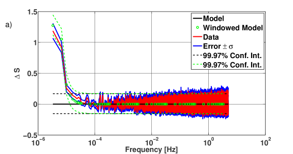
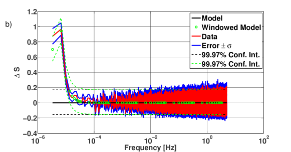
$\Delta S$ is calculated for the simulated data and the windowed model with respect to the reference model. Results are reported in figure 6. A $99.97\%$ confidence interval is calculated on the basis of the statistical properties of $\Delta S$.

The effect of the window on the spectra calculation is noticeably high on the first $3$ frequency bins, where the deviation from the reference model exceeds the confidence interval. In addition, it is clearly observable up to the $10^{th}$ bin. The windowed model and the simulated data are consistent on the basis of the chosen confidence region.

A considerable number of data points, especially at high frequencies, lie outside the confidence levels, and it is of fundamental importance to assess if such outliers are caused by the random nature of the data, or if they come from systematic errors in the spectral estimation or data generation processes. The confidence levels at $99.97\%$ define a region in which the data are expected to lie with that probability. This also means that in $0.03\%$ of the observations an outlier can be observed. As we are dealing with datasets of $1.5\times 10^{6}$ points the number of expected outliers is high.

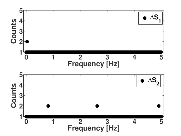
In order to distinguish between systematic outliers and statistical outliers the averaging process over $500$ independent realizations was repeated $5$ times and the frequencies at which the values of $\Delta S$ were outside the defined confidence interval were recorded. The first $10$ frequency bins are excluded from the numbering because they are systematically affected by the spectral widow effect. Figure 7 reports a histogram of the cumulative count of the outliers frequencies for the $5$ different realizations. If an outlier is originated by a systematic error, then it is expected to be counted $5$ times. As can be observed from figure 7, the maximum value obtained is $2$ for both channels; this is a definitive indication of the statistical nature of the observed outliers.

Figure 6: $\Delta S\left(\omega\right)$ calculated for a) First channel and b) Second channel. Simulated results are compared with the model expectation and the windowed model expectation. A $99.97\%$ confidence interval is calculated for quantitative comparison with the models.

Figure 7: Histogram of the outliers frequencies for $\Delta S_{1}$ and $\Delta S_{2}$.

As stated above, the correlation properties of the data series can be explored with the sample coherence calculated as in equation (48). Power spectra and cross-spectrum were estimated with the averaged Welch periodogram method using a 4-term Blackman-Harris window over 145 data segments $6\times 10^{4}$ points long. The separate 500 realizations are then averaged and, assuming the averaged process is approximately normally distributed, the error on the estimation is calculated as described above. Results are reported in figure 8 and compared with the expectation from the reference model. Since the coherence is constructed from a ratio between cross-spectrum and power spectra the effect of the window on the lowermost frequency bins is strongly attenuated.

(a)

(b)

Figure 8: Averaged cross-coherence compared with the reference model. a) Real part. b) Imaginary part.

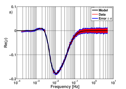
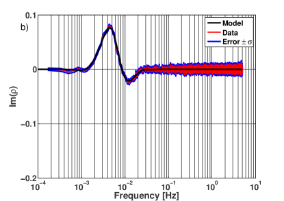
The simulated data (averaged over $500$ realizations) and the reference model are in satisfactory agreement within the tolerance region defined by the uncertainty. On the basis of the above discussion, the oscillations observed in the coherence curves (figure 8) can be associated with the statistical fluctuations caused by the random nature of the data.

IV Conclusions

A robust procedure for the generation of multichannel stationary noise with a given cross-spectral matrix is reported. Based on some assumptions on the noise sources acting on the system under study, an expected model for the cross-spectral matrix of the multichannel output noise can be developed. From such a model the noise coloring filters are identified by an eigendecomposition of the cross-spectral matrix (frequency by frequency) and a frequency domain fit procedure. A multichannel colored noise data series can then be generated from a multichannel $\delta$ correlated random noise process provided that the recurrence equations are properly initialized in order to avoid transients at the beginning of the noise sequence. It is demonstrated that the only source of systematic errors in the process is associated with the fit procedure. On the other hand, the accuracy of the fit can be increased at the expense of the computational cost of the whole process; this, in principle, ensures that the process reaches the desired accuracy. An average over $500$ independent realizations of the multichannel noise process has demonstrated the statistical consistency between generated noise and the reference model if the effect of the spectral window is taken into account. Oscillations in the averaged spectra with respect to the model can be unambiguously attributed to statistical fluctuations. The analysis reported demonstrates that the tool can be applied for the calibration of spectral estimators in experiments where noise spectral energy content must be estimated with very high accuracy, as is the case for the LTP experiment. MATLAB based algorithms are available for free download at the LTPDA project web page.

V References

References

- (1) M. Armano et al., Class. Quantum Grav. 26, 094001 (2009).
- (2) S. Anza et al., Class. Quantum Grav. 22, S125ñ38 (2005).
- (3) P. McNamara, S Vitale and K Danzmann, Class. Quantum Grav. 25, 114034 (2008).
- (4) D. Bortoluzzi et al., Class. Quantum Grav. 21, S573 (2004).
- (5) D. Bortoluzzi et al., Class. Quantum Grav. 20, S89 (2003).
- (6) S. Stein and J. E. Storer, IRE Trans. Inform. Theory 2, 87 (1956).
- (7) J. M. Levin, IRE Trans. on Information Theory IT-6, 545 (1960).
- (8) S. M. Kay, Proc. IEEE 69, 481 (1981).
- (9) J. N. Franklin, SIAM Rev. 7, 68 (1965).
- (10) D. B. Percival and A. T. Walden, Spectral analysis for physical applications (Cambridge University Press, 1998), p. 98.
- (11) A. Papoulis, Signal Analysis (New York, McGraw-Hill, 1977), p. 53.
- (12) S. M. Kay, Modern Spectral Estimation: Theory and Application (Prentice-Hall signal processing series, 1988), p. 446.
- (13) A. Monsky et al., Class. Quantum Grav. 26, 094004 (2009).
- (14) M. Hewitson et al., Class. Quantum Grav. 26, 094003 (2009).
- (15) L. Ferraioli, M. Hueller and S. Vitale, Class. Quantum Grav. 26, 094013 (2009).
- (16) B. Gustavsen and A. Semlyen, IEEE Trans. Power Delivery 14, 1052 (1999).
- (17) B. Gustavsen, IEEE Trans. Power Delivery 21, 1587 (2006).
- (18) Y. S. Mekonnen and J. E. Schutt-Aine, in Proceedings of the 58th Electronic Components and Technology Conference (27-30 May, 2008), p. 1231.
- (19) MATLAB http://www.mathworks.com
- (20) LTPDA: a MATLAB toolbox for accountable and reproducible data analysis http://www.lisa.aeihannover.de/ltpda
- (21) F. J. Harris, Proc. IEEE 66, 51 (1978).
- (22) G. M. Jenkins and D. G. Watts, Spectral Analysis and Its Applications (San Francisco, CA: Holden-Day, 1968), p. 255.