“TNOs are cool”: A survey of the trans-neptunian region

Thermal emission from Kuiper Belt object (136108) Haumea was measured with Herschel–PACS at 100 $\mu$m and 160 $\mu$m for almost a full rotation period. Observations clearly indicate a 100 $\mu$m thermal lightcurve with an amplitude of a factor of $\sim$ 2, which is positively correlated with the optical lightcurve. This confirms that both are primarily due to shape effects. A 160 $\mu$m lightcurve is marginally detected. Radiometric fits of the mean Herschel- and Spitzer- fluxes indicate an equivalent diameter D$\sim$1300 km and a geometric albedo p_v$\sim$0.70-0.75. These values agree with inferences from the optical lightcurve, supporting the hydrostatic equilibrium hypothesis. The large amplitude of the 100 $\mu$m lightcurve suggests that the object has a high projected a/b axis ratio ($\sim$1.3) and a low thermal inertia as well as possible variable infrared beaming. This may point to fine regolith on the surface, with a lunar-type photometric behavior. The quality of the thermal data is not sufficient to clearly detect the effects of a surface dark spot.

1 Introduction

The dwarf planet (136108) Haumea (formerly 2003 EL₆₁) is one of the most remarkable transneptunian objects (TNOs). Its large amplitude visible lightcurve indicates a very short ($\sim$3.91 h) rotation period and considerable rotational deformation, with semi-major axes estimated to be 1000$\times$800$\times$500 km (Rabinowitz et al. 2006). It is one of the bluest TNOs (Tegler et al. 2007), and unlike other 1000 km-scale TNOs, its surface is covered by almost pure water ice (Trujillo et al. 2007), though its high density ($\sim$2.6 g cm^-3, Lacerda and Jewitt 2007) indicates a more rocky interior. It possesses two satellites (Brown et al. 2006), the larger of which is also water-ice coated (Barkume et al. 2006). All this, and the observation that several TNOs with similar orbital parameters also show evidence of surface water ice (Schaller and Brown 2008), point to Haumea being the largest remnant of a massive ancient ($>$1 Gyr) collision (Ragozzine and Brown 2007). High time-resolution, multi-color, photometry provides evidence for a surface feature redder and darker than the surrounding materials (Lacerda et al. 2008, Lacerda 2009), perhaps of collisional origin, and makes Haumea the second TNO (after Pluto) with surface heterogeneity. Both Spitzer thermal observations (Stansberry et al. 2008) and visible photometry indicate that Haumea is one of the most reflective TNOs (estimated geometric albedo 0.6 – 0.85).

Except for near-Earth asteroids (e.g. Harris et al. 1998, Müller et al. 2005), thermal lightcurves of airless bodies are available only for a few objects. In combination with the optical lightcurve, they provide a means to distinguish between the effects of shape and surface markings and to infer thermal properties of the surface. Lockwood and Brown (2009) reported on the detection of Haumea’s lightcurve at 70 $\mu$m with Spitzer. We present here observations of Haumea at 100 and 160 $\mu$m with Herschel-PACS, performed in the framework of the Open Time Key Program “TNOs are cool” (Müller et al. 2009, 2010).

2 Herschel / PACS observations

2.1 Observations and data reduction

Haumea was observed with the PACS photometer (Poglitsch et al. poglitsch10 (2010)) of Herschel (Pilbratt et al. 2010) on 2009, December 23 and 25 (Obs. ID # 1342188470 and # 1342188520, respectively), using the 100 $\mu$m (“green”) / 160 $\mu$m (“red”) combination. We used a mini scan-map mode which homogeneously covered a field roughly 1 arcmin in diameter (Müller et al. 2010).

Although our observations on December 23 were initially designed to cover 110 % of Haumea’s visible lightcurve, they lasted only 3.36 hr (i.e. 86 % of the 3.91 hr period) end-to-end (UT 5:52:01–9:13:25) due to shorter than expected observations overheads in the mini-scan mode. Observations on December 25 lasted only 40 minutes (UT 6:13:39–6:53:59). Their goal was to verify the measured target flux at a given rotational phase against a different sky background (Haumea moved by about 85” between these two dates).

The whole observation sequence for December 23 consisted of 400 individual measurement subscans. As a compromise between temporal resolution and sensitivity, we divided the sequence into ten, $\sim$20-min long blocks (40 subscans each) for the 100 $\mu$m data and into five, $\sim$40-min blocks (80 subscans each) at 160 $\mu$m. Similarly, the 40 individual subscans of December 25 were combined into two blocks at 100 $\mu$m and one single block at 160 $\mu$m. Individual measurements were reduced with standard scan map processing, applying masked high pass filtering in the vicinity of bright sources (only Haumea was notably bright in the central region of the maps) and resampling maps with pixel sizes of 1” in the green and 2” in the red. For the high-pass filter we used widths of 15” and 20” for the green and red bands, respectively. The selection criterion for the mask was set to be the 3 $\sigma$ value of the image. The calibration was done in a standard way, applying flux overestimation corrections of 1.09 and 1.29 at 100 and 160 $\mu$m, respectively, as recommended at the time of the processing (PICC-ME-TN-036, 22-Feb-2010, see herschel.esac.esa.int). Color corrections (to monochromatic reference wavelengths of 100.0 and 160.0 $\mu$m) are at the 1 % level, i.e. negligible in view of other uncertainties.

Figure 1: Photometry and associated uncertainties in 100-$\mu$m band. Aperture-corrected curves-of-growth are shown for the two visits of Dec. 23 corresponding to lightcurve maximum and minimum. The orange and red curves are for measurements uncorrected for sky contribution. The other curves are for sky-corrected measurements, with the sky contribution estimated in annuli centered on Haumea and with various internal and external radii (r_int = 16-56” and r_ext = r_int + 10”).

2.2 Photometry

For each visit to Haumea, we performed standard aperture photometry with the IRAF/Daophot flux extraction routines and aperture correction technique (Howell 1989). We constructed photometric curves of growth, using aperture radii ranging from 1” to 15”, and performed aperture corrections based on tables of the fraction of the encircled energy of a point source. The optimum aperture for photometry was selected from inspection of the curves of growth, and was usually found to be 1.0-1.25 times the PSF FWHM (7.7” in the green and 12” in the red) in radius, and to lie in the “plateau” zone of the curves of growth. In determining the “optimized” source flux in this manner, we did not subtract any sky contribution, as the latter is normally eliminated in the data reduction process. However, to assess the uncertainty on this flux value, we also constructed sky-subtracted curve-of-growths, selecting a variety of regions of the image (typically annuli centered on the source) to measure the sky contribution. This method is illustrated in Fig. 1 for two of the 100 $\mu$m visits to Haumea, corresponding to the maximum and minimum fluxes. The standard deviation in all flux values determined in this manner and for a broad range of aperture radii (3”–15”) finally provided the 1$\sigma$ uncertainties attached to the flux measurements.

3 Phasing with visible observations

We observed Haumea in the visible on 2010 January 20, 21, 23, and 26, using a 0.4 m f/3.5 telescope located in San Pedro de Atacama (Chile) and equipped with a 4008 x 2672 CCD camera. A broad band filter (390-700nm) was used with integration times of 300 s. Additional data were acquired on 2010 January 28, with the 1.2 m telescope at Calar Alto Observatory (Spain), equipped with a 2k$\times$2k CCD camera in the R filter, again with 300 s integration times. The same reference stars were consistently observed each night. Observations were reduced and analyzed as in Ortiz et al. (2007), with some refinements described in Thirouin et al. (2010). The 3.92 hr period, 0.28 mag amplitude lightcurve was readily detected, and by combining these data with the Lacerda et al. (2008) observations, an improved rotation period of 3.915341$\pm$0.000005 h was derived. This allowed us to phase the January 2010 observations back to the time of the Herschel observations very accurately.

4 Results and analysis

4.1 Thermal lightcurve

The measured Haumea fluxes on Dec. 23 (10 points at 100 $\mu$m, 5 points at 160 $\mu$m) are plotted in Fig. 2 as a function of fractional date. At 100 $\mu$m a clear lightcurve is detected, with mean $\sim$25 mJy flux and high contrast (18-35 mJy, i.e. almost a factor of 2 peak-to-peak), while a more marginal lightcurve is determined at 160 $\mu$m. Superimposed on Fig. 2 are the fluxes measured on Dec. 25 (2 points at 100 $\mu$m, 1 point at 160 $\mu$m), rephased to Dec. 23 using the 3.915341 h period. Their agreement with the Dec. 23 measurements demonstrates the robustness of the lightcurve. To further verify the large amplitude and overall structure of the 100 $\mu$m lightcurve, we also performed “differential photometry”, subtracting the median or averages of all combined images of Dec. 23 from each individual image. This confirmed a peak-to-peak lightcurve amplitude of $\sim$17 mJy in the green.

Overall, the 100 $\mu$m lightcurve appears positively correlated with the visible lightcurve, as expected if shape effects are dominant. Nonetheless, the secondary peak (near JD2455188.843) and absolute minimum (JD2455188.883) of the visible lightcurve, attributed to the presence of a dark spot (Lacerda et al. 2008) are also associated with a secondary maximum and minimum in the thermal lightcurve. If anything, the dark spot should be warmer than the rest of the surface, and therefore tend to enhance the thermal emission. This is observed for the secondary minimum but the secondary peak shows the opposite behavior. We qualitatively conclude that the thermal lightcurve confirms the elongated shape of Haumea, but does not unambiguously support the presence of a spot.

Figure 2: Observed thermal lightcurve of Haumea at 100 $\mu$m (green) and 160 $\mu$m (red). Black dots show the visible lightcurve (H_V, right scale); the enhanced part corresponds to the fraction affected by the presence of the dark spot in the Lacerda et al. (2008) model.

4.2 Radiometric size and albedo

We first performed radiometric modeling of the mean fluxes, combining the mean 100 and 160 $\mu$m fluxes (25$\pm$2 mJy and 21$\pm$3 mJy, respectively) with Spitzer results at 24 and 70 $\mu$m (Stansberry et al. 2008). The latter indicate a color-corrected flux of 13.4$\pm$2.0 mJy at 71.42 $\mu$m and upper limit of 0.025 mJy at 23.68 $\mu$m, for measurements performed on 2005 June 22, UT = 9:11-9:40, roughly mid-way between visible lightcurve maximum and minimum. (Note that the 7.7 mJy value published in Stansberry et al. (2008) is the average of the above with a much lower flux (2.5 mJy) measured on 2005 June 20; we suspect this latter observation was compromised).

Modeling was performed along the NEATM approach (Harris et al., 1998, Müller et al. 2010), a.k.a. the “hybrid-STM” (Stansberry et al. 2008). Essentially, the temperature distribution across the object follows instantaneous equilibrium with local insolation, but is modified by an empirical factor $\eta^{-1/4}$, where $\eta$, the beaming parameter, can be either specified or fit to the data. In this framework $\eta$ values much higher than 1 indicate large thermal inertia effects, while $\eta$$\leq$1 points to low thermal inertia and important surface roughness. Free parameters are the mean radiometric diameter D, geometric albedo p_v, and possibly $\eta$. We used a mean H_R = 0.09 and V–R = 0.335, i.e a mean H_V = 0.425. We adopted a phase integral q = 0.7, intermediate between those estimated for Pluto (0.8) and Charon (0.6) (Lellouch et al. 2000), and an emissivity $\epsilon$ = 0.9. We considered three cases: $\eta$ = 1, $\eta$ = 1.2 (mean value inferred for TNOs by Stansberry et al. 2008), and free $\eta$. Table 1 gives the radiometric solution for the three cases, and Fig. 3 shows the associated fits. A satisfactory match of the 70, 100 and 160 $\mu$m fluxes is achieved in all cases, though it is noteworthy that (i) when $\eta$ is a fitting parameter, it is poorly constrained and (ii) the predicted 24 $\mu$m is always essentially at the Spitzer upper limit. Note that using the “default” q value for TNOs (0.39) would lead to p_v $\sim$1, which is strongly at odds with the observed correlation between p_v and q (Lellouch et al. 2000).

Table 1: Radiometric fits for (136108) Haumea

Model	$\eta$	D(km)	pv	Reduced $\chi^{2}$
Fixed $\eta$	1.0	1230$\pm$18	0.810$\pm$0.024	1.14
Fixed $\eta$	1.2	1276$\pm$20	0.752$\pm$0.024	1.08
Free $\eta$	1.38$\pm$0.71	1324$\pm$167	0.698 $\pm$0.189	1.06

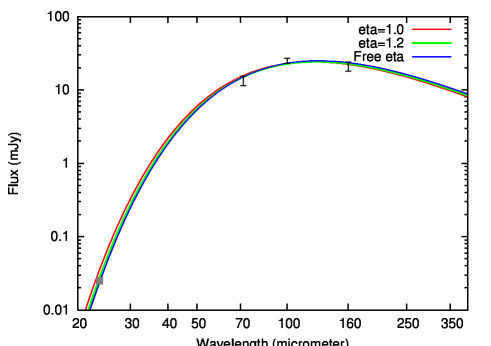
Figure 3: Approximate Haumea SED measured from Herschel/PACS (100 and 160 $\mu$m) and Spitzer (24 and 70 $\mu$m). The grey square at 23.68 $\mu$m is the Spitzer upper limit. Model fits using NEATM with fixed $\eta$ ($\eta$ = 1.0 and $\eta$ = 1.2 are shown) and free $\eta$ (best fit $\eta$ = 1.38) are shown.

4.3 Modeling of the thermal lightcurve

Figure 4: Fits of Haumea 100 $\mu$m and 160 $\mu$m lightcurves with shape models 1 and 2 (see text) and different distributions of $\eta$. Green curves: constant $\eta$ (1.15, for both models). Blue curves: Variable $\eta$ as a function of longitude $L$. For model 1, $\eta$ = 0.40 at $L$ = 80–130, $\eta$ = 1.6 at $L$ = 130–180, and $\eta$ = 1.15 elsewhere. For model 2, $\eta$ = 0.52 at $L$ = 130–180 and $\eta$ = 1.15 elsewhere. Red curves: constant $\eta$, but a dark spot is included. The spot covers longitudes from 292.5^∘ to 337.5^∘, i.e. 1/4 of one hemisphere, and its albedo is taken as 0.59 (model 1) or 0.56 (model 2). The adopted reference longitude system is shown, in which 0^∘ is the semi-minor axis closest to the spot.

To model the 100 $\mu$m and 160 $\mu$m lightcurves, the above model was modified to account for Haumea’s elongated shape. For that purpose we used a versatile tool called OASIS, the Optimized Astrophysical Simulator for Imaging Systems (Jorda et al. 2010), describing the object as an ellipsoid made of 5120 triangles. OASIS then calculates the orientation of each triangle relative to (i) pole orientation, (ii) observer position, (iii) Sun position, and (iv) time as the object rotates. The large amplitude of Haumea’s lightcurve favors a large aspect angle. We nominally used OASIS assuming an equator-on object (aspect angle $\theta$ = 90^∘) and with the observer at the Sun (phase angle = 0^∘), but given the orbits of Haumea’s satellites (Ragozzine and Brown 2009), we also considered $\theta$ = 75^∘. The direction of the Sun dictated the local insolation, which was then fed into the NEATM model. Input parameters for Haumea were the three semi-major axes (a, b, c) and the geometric albedo (p_v). Those were derived following Rabinowitz et al. (2006) and Lacerda and Jewitt (2007), but using the measurements of Lacerda et al. (2008). Essentially the amplitude and period of the visible lightcurve, and the assumption of a Jacobi figure (hydrostatic equilibrium) provide b/a, c/a and the density $\rho$. Knowledge of Haumea’s mass (4.0$\times$10²¹ kg; Ragozzine and Brown 2009) then provides the absolute semi-major axes. Finally, p_v is deduced from H_V.

We first used the preferred photometric solution of Lacerda et al. (2008), in which a Lambert scattering law is assumed, expected for high-albedo icy surfaces. For $\theta$ = 90^∘, this yields b/a = 0.87, c/a = 0.54, and $\rho$ = 2.55 g cm^-3. In this case, a = 927 km, b = 807 km, c = 501 km, and p_v = 0.74 (model 1). We also used an alternative model with a higher axial ratio, as inferred for a lunar-type Lommel-Seelinger reflectance function. In this case, and still with $\theta$ = 90^∘, b/a = 0.80, c/a = 0.52, $\rho$= 2.59, a = 961 km, b = 768 km, c = 499 km, and p_v = 0.71 (model 2). We emphasize that the equivalent mean diameter, which can be taken as 2a^1/4b^1/4c^1/2 is 1309–1317 km, in excellent agreement with the above radiometric fits; the same comment applies for p_v (see Table 1). This tends to support the hydrostatic equilibrium hypothesis. Once the object dimensions and albedo are fixed, the only free parameter for the thermal model is $\eta$.

For $\theta$ =90^∘, Fig. 4 shows that model 1 with $\eta$ = 1.15 reproduces the mean flux level, but the amplitude of the 100 $\mu$m lightcurve is grossly underestimated. Model 2, again with $\eta$ = 1.15, provides a good fit to the 100 $\mu$m data, especially in the region of the secondary maximum near JD2455188.843, but the $\sim$35 mJy main peak near JD2455188.763 is still underpredicted. We explored models with spatially variable $\eta$ to try and fit this peak. These models required an extended region with much lower $\eta$ ($\eta$ = 0.40 and 0.52 for models 1 and 2, respectively). For model 1, fitting the overall lightcurve structure would even require a three-terrain $\eta$ model. $\eta$ values below 0.6 imply r.m.s. slopes well in excess of 40^∘ (Spencer 1990, Lagerros, 1998) and seem unrealistic for this object. Yet our result might qualitatively point to a highly craterized region with extremely strong beaming, given the very high surface albedo. Further thermophysical modeling, including a more realistic description of surface roughness, is required. Note finally that models with $\theta$ = 75^∘ gave similar results as $\theta$ = 90^∘, provided slightly higher $\eta$ values were used (e.g. $\eta$ = 1.35 instead of 1.15 for the uniform model).

We finally investigated the effect of a dark spot on the surface at the location inferred by Lacerda et al. (2008) (i.e. centered at 315^∘ in the longitude system of Fig. 4). It was prescribed to cover 1/4 of Haumea’s maximum projected cross section, with a relative albedo constrained by the Lacerda et al. (their Fig. 7) results. Other combinations of spot coverage / relative albedo did not qualitatively change the results. As expected, the dark spot enhances the thermal flux in the relevant longitude ranges, but our data are insufficient to demonstrate its effect.

Besides the determination of Haumea’s diameter and albedo, the essential finding is that the large amplitude of the thermal lightcurve implies both a high a/b ratio ($\sim$1.3) and a low $\eta$ ($<$1.15-1.35, depending on spin orientation) value, indicative of a low thermal inertia. This seems inconsistent with compact water ice at $\sim$40 K, and rather points to a porous surface. As a high a/b ratio also implies a lunar-like photometric behavior, this could point to Haumea’s surface being covered with loose regolith with poor thermal conductivity. The same conclusion is reached for other objects in our sample, such as the Plutino 2003 AZ₈₄ and Centaur 42355 Typhon (Müller et al. 2010). Surface regolith may be produced by collision events and retained on the surface of large TNOs.

References

- Barkume et al. (2006) Barkume, K. M., Brown, M. E., & Schaller, E. L. 2006, ApJL, 640, L87
- Brown et al. (2006) Brown, M. E., et al. 2006, ApJL, 639, L43
- Harris et al. (1998) Harris, A. W., Davies, J. K., & Green, S. F. 1998, Icarus, 135, 441
- Howell (1989) Howell, S. B. 1989, PASP, 101, 616
- (5) Jorda, L., et al. 2010, SPIE, submitted
- Lacerda & Jewitt (2007) Lacerda, P., & Jewitt, D. C. 2007, AJ, 133, 1393
- Lacerda et al. (2008) Lacerda, P., Jewitt, D., & Peixinho, N. 2008, AJ, 135, 1749
- Lacerda (2009) Lacerda, P. 2009, AJ, 137, 3404
- Lagerros (1998) Lagerros, J.S.V., A & A, 332, 1123
- Lellouch (00) ellouch, E. et al. 2000 Icarus, 147, 220
- Lockwood& Brown (2009) Lockwood, A., & Brown, M. E. 2009, Bull. Amer. Astron. Soc., 41, #65.06
- Müller et al. (2005) Müller, T. G., et al. 2005, A&A, 443, 347
- (13) Müller, T. G et al. 2009, Earth, Moon, and Planets, 105, 209-219.
- (14) Müller, T. G. et al., 2010, this volume.
- Ortiz et al. (2007) Ortiz, J. L., et al. 2007, A&A, 468, L13
- (16) Pilbratt, G. et al. 2010, this volume.
- (17) Poglitsch, A. et al. 2010, this volume.
- Rabinowitz et al. (2006) Rabinowitz, D. L., et al. 2006, ApJ, 639, 1238
- Ragozzine & Brown (2007) Ragozzine, D., & Brown, M. E. 2007, AJ, 134, 2160
- Ragozzine & Brown (2009) Ragozzine, D., & Brown, M. E. 2009, AJ, 137, 4766
- Schaller & Brown (2008) Schaller, E. L., & Brown, M. E. 2008, ApJL, 684, L107
- Spencer (90) Spencer, J.R., 1990, Icarus 83, 27
- Stansberry et al. (2008) Stansberry, J., et al. 2008, in: The Solar System Beyond Neptune, University of Arizona press, pp. 161.
- Tegler et al. (2007) Tegler, S. C., et al. 2007, AJ, 133, 526
- Thirouin et al. (2010) Thirouin, A., et al. 2010, A & A, in press.
- Trujillo et al. (2007) Trujillo, C. A., 2007, ApJ, 655, 1172