SFB/CPP-10-34 TTP/10-23 HU-EP-10/25 WUB/10-13
Light MSSM Higgs boson mass to three-loop accuracy

P. Kant(a), R.V. Harlander(b), L. Mihaila(c), M. Steinhauser(c)
(a) Institut für Physik, Humboldt-Universität zu Berlin
12489 Berlin, Germany
(b) Fachbereich C, Theoretische Physik, Universität Wuppertal
42097 Wuppertal, Germany
(c) Institut für Theoretische Teilchenphysik, Karlsruhe Institute of Technology (KIT)
76128 Karlsruhe, Germany
Abstract

The light CP even Higgs boson mass, Mhsubscript𝑀M_{h}, is calculated to three-loop accuracy within the Minimal Supersymmetric Standard Model (MSSM). The result is expressed in terms of DR¯¯DR\overline{\mbox{DR}} parameters and implemented in the computer program H3m. The calculation is based on the proper approximations and their combination in various regions of the parameter space. The three-loop effects to Mhsubscript𝑀M_{h} are typically of the order of a few hundred MeV and opposite in sign to the two-loop corrections. The remaining theory uncertainty due to higher order perturbative corrections is estimated to be less than 1 GeV.

PACS numbers: 12.60.Jv, 14.80.Da, 12.38.Bx

1 Introduction

Among the main expectations in view of the CERN Large Hadron Collider (LHC) is to provide clear phenomena beyond the Standard Model (SM) of particle physics. A very promising candidate for an extension of the SM is the so-called Minimal Supersymmetric Standard Model (MSSM) which relies on an extended symmetry between fermions and bosons [2, 3]. It is constructed in such a way that in the low-energy limit the SM is recovered thus leading to the same phenomena in the energy range around the electroweak scale. In particular, the MSSM is in accordance with the electroweak precision data [4]. At the same time it provides a dark matter candidate, solves the hierarchy problem and provides a platform where also gravitational interactions can be included.

An appealing feature of the MSSM is the quite restrictive Higgs sector which is described at leading order by two independent parameters. In particular, the mass of the lightest CP-even Higgs boson, Mhsubscript𝑀M_{h}, is not a free parameter, like in the SM, but a prediction which can be used in order to test this minimal supersymmetric extension of the SM.

Mhsubscript𝑀M_{h} is very sensitive to radiative corrections. In lowest order it is bound from above by the Z𝑍Z boson mass which is already excluded by experiment. Already quite some time ago it has been observed that large one-loop corrections, in particular from the top quark and top squark sector can raise Mhsubscript𝑀M_{h} to about 140 GeV [5, 6, 7]. In the meantime a number of higher order corrections have been computed including even CP-violating couplings and improvements from renormalization group considerations (see Refs. [8, 9, 10] for a review). In this paper we consider neither CP violation nor the resummation of higher order logarithms. Let us nevertheless mention that in particular CP violating phases can lead to a shift of a few GeV in Mhsubscript𝑀M_{h}, see, e.g., Refs. [Heinemeyer:2007aq, Carena:2000yi]. In Ref. [11] a large class of two-loop corrections to the lightest Higgs boson mass have been considered and in Ref. [12] leading logarithmic corrections at three-loop order have been computed. The first complete three-loop calculation of the leading quartic top quark mass terms within supersymmetric QCD (SQCD; more precisely, this means supersymmetric six-flavor QCD coupled to the MSSM Higgs sector) has been performed in Ref. [13] for a degenerate supersymmetric mass spectrum. It is the aim of this paper to provide details and extend this calculation.

At the moment there are two computer programs publicly available which include most of the higher order corrections. FeynHiggs has been available already since 1998 [14, 15, 10] and has been continuously improved since then [16, 17]. In particular, it contains all numerically important two-loop corrections and accepts both real and complex MSSM input parameters. The second program, CPSuperH [18, 19], is based on a renormalization group improved diagrammatic calculation and allows for explicit CP violation. Both programs compute the mass spectrum as well as the decay width of the neutral and charged Higgs bosons.

In this paper we discuss the three-loop corrections originating from the strong sector of the MSSM which are proportional to the quartic top quark mass. At three-loop order several mass scales enter the Feynman diagrams making their evaluation quite involved. In addition to the top quark mass there are the top squark masses, the gluino mass and the masses of the remaining squarks. An exact evaluation of the three-loop integrals is currently out of range. However, it is possible to apply expansion techniques for various limits which allow to cover a large part of the supersymmetric (SUSY) parameter space. In particular, we can construct precise approximations for the Snowmass Points and Slopes (SPS) [20, 21]. Our set-up is easily extendable to other regions of parameter space which may become interesting in future.

Together with this paper we provide a Mathematica program, H3m [22], which contains all our three-loop results. Furthermore, H3m constitutes an interface to FeynHiggs [23] and various SUSY spectrum generators which allows for precise predictions of Mhsubscript𝑀M_{h} on the basis of realistic SUSY scenarios.

The remainder of the paper is organized as follows: In the next Section we revisit the two-loop corrections. In particular, we construct approximations which are also available at three-loop order and compare with the exact result. In Section 3 we provide details on our three-loop calculations for the various hierarchies. In particular we discuss the renormalization and the asymptotic expansion. Section 4 describes the implementation of our results in the computer program H3m and the phenomenological implementations are discussed in Section 5. We present a summary and the conclusions in Section 6. In the Appendices additional material is provided, in particular all the one- and two-loop counterterms that have entered in our calculation.

2 Mhsubscript𝑀M_{h} in the MSSM

2.1 Higgs boson sector of the MSSM

The mass of the Higgs boson is obtained from the quadratic terms in the corresponding potential which for the MSSM has the following form:

VHsubscript𝑉𝐻\displaystyle V_{H} =(|μSUSY|2+m12)|H1|2+(|μSUSY|2+m22)|H2|2absentsuperscriptsubscript𝜇SUSY2superscriptsubscript𝑚12superscriptsubscript𝐻12superscriptsubscript𝜇SUSY2superscriptsubscript𝑚22superscriptsubscript𝐻22\displaystyle=\left({\left\lvert{\mu_{\rm{SUSY}{}}}\right\rvert}^{2}+m_{1}^{2}\right){\left\lvert{H_{1}}\right\rvert}^{2}+\left({\left\lvert{\mu_{\rm{SUSY}{}}}\right\rvert}^{2}+m_{2}^{2}\right){\left\lvert{H_{2}}\right\rvert}^{2}
m122(ϵabH1aH2b+ϵabH1aH2b)superscriptsubscript𝑚122subscriptitalic-ϵ𝑎𝑏superscriptsubscript𝐻1𝑎superscriptsubscript𝐻2𝑏subscriptitalic-ϵ𝑎𝑏superscriptsuperscriptsubscript𝐻1𝑎superscriptsuperscriptsubscript𝐻2𝑏\displaystyle-m_{12}^{2}\left(\epsilon_{ab}H_{1}^{a}H_{2}^{b}+\epsilon_{ab}{H_{1}^{a}}^{*}{H_{2}^{b}}^{*}\right)
+18(g12+g22)[|H1|2|H2|2]2+12g22|H1H2|2.18superscriptsubscript𝑔12superscriptsubscript𝑔22superscriptdelimited-[]superscriptsubscript𝐻12superscriptsubscript𝐻22212superscriptsubscript𝑔22superscriptsuperscriptsubscript𝐻1subscript𝐻22\displaystyle+\frac{1}{8}\left(g_{1}^{2}+g_{2}^{2}\right)\left[{\left\lvert{H_{1}}\right\rvert}^{2}-{\left\lvert{H_{2}}\right\rvert}^{2}\right]^{2}+\frac{1}{2}g_{2}^{2}{\left\lvert{H_{1}^{\dagger}H_{2}}\right\rvert}^{2}\,. (1)

with ϵ12=ϵ21=1subscriptitalic-ϵ12subscriptitalic-ϵ211\epsilon_{12}=-\epsilon_{21}=1 and ϵ11=ϵ22=0subscriptitalic-ϵ11subscriptitalic-ϵ220\epsilon_{11}=\epsilon_{22}=0. μSUSYsubscript𝜇SUSY\mu_{\rm SUSY} is the Higgs-Higgsino bilinear coupling from the super potential and m1,m2subscript𝑚1subscript𝑚2m_{1},m_{2} and m12subscript𝑚12m_{12} are soft breaking parameters. Note that the quartic terms are fixed by the SU(2) and U(1) gauge couplings g1subscript𝑔1g_{1} and g2subscript𝑔2g_{2}. The parameters in (1) are related to the masses of the gauge bosons and the pseudoscalar Higgs via

MW2=12g22(v12+v22),MZ2=12(g12+g22)(v12+v22),MA2=m122(tanβ+cotβ),formulae-sequencesuperscriptsubscript𝑀𝑊212superscriptsubscript𝑔22superscriptsubscript𝑣12superscriptsubscript𝑣22formulae-sequencesuperscriptsubscript𝑀𝑍212superscriptsubscript𝑔12superscriptsubscript𝑔22superscriptsubscript𝑣12superscriptsubscript𝑣22superscriptsubscript𝑀𝐴2superscriptsubscript𝑚122𝛽𝛽\begin{split}M_{W}^{2}&=\frac{1}{2}g_{2}^{2}\left(v_{1}^{2}+v_{2}^{2}\right),\\ M_{Z}^{2}&=\frac{1}{2}\left(g_{1}^{2}+g_{2}^{2}\right)\left(v_{1}^{2}+v_{2}^{2}\right),\\ M_{A}^{2}&=-m_{12}^{2}\left(\tan\beta+\cot\beta\right)\,,\end{split} (2)

where tanβ=v2/v1𝛽subscript𝑣2subscript𝑣1\tan\beta=v_{2}/v_{1}.

After spontaneous symmetry breaking the neutral components of the doublets H1subscript𝐻1H_{1} and H2subscript𝐻2H_{2} acquire the vacuum expectation values v1subscript𝑣1v_{1} and v2subscript𝑣2v_{2}, and we write

H1subscript𝐻1\displaystyle H_{1} =(v1+12(ϕ1+iχ1)ϕ1),absentmatrixsubscript𝑣112subscriptitalic-ϕ1𝑖subscript𝜒1superscriptsubscriptitalic-ϕ1\displaystyle=\begin{pmatrix}v_{1}+\frac{1}{\sqrt{2}}\left(\phi_{1}+i\chi_{1}\right)\\ -\phi_{1}^{-}\end{pmatrix}\,,
H2subscript𝐻2\displaystyle H_{2} =(ϕ2+v2+12(ϕ2+iχ2)),absentmatrixsuperscriptsubscriptitalic-ϕ2subscript𝑣212subscriptitalic-ϕ2𝑖subscript𝜒2\displaystyle=\begin{pmatrix}\phi_{2}^{+}\\ v_{2}+\frac{1}{\sqrt{2}}\left(\phi_{2}+i\chi_{2}\right)\end{pmatrix}\,, (3)

which leads to the following representation of the Higgs boson mass matrix at tree level:

H,tree2superscriptsubscript𝐻tree2\displaystyle{\cal M}_{H,\rm tree}^{2} =\displaystyle\!=\! 122Vϕ1ϕ2=sin2β2(MZ2cotβ+MA2tanβMZ2MA2MZ2MA2MZ2tanβ+MA2cotβ),12superscript2𝑉subscriptitalic-ϕ1subscriptitalic-ϕ22𝛽2superscriptsubscript𝑀𝑍2𝛽superscriptsubscript𝑀𝐴2𝛽superscriptsubscript𝑀𝑍2superscriptsubscript𝑀𝐴2superscriptsubscript𝑀𝑍2superscriptsubscript𝑀𝐴2superscriptsubscript𝑀𝑍2𝛽superscriptsubscript𝑀𝐴2𝛽\displaystyle\frac{1}{2}\frac{\partial^{2}V}{\partial\phi_{1}\partial\phi_{2}}=\frac{\sin 2\beta}{2}\left(\begin{array}[]{cc}M_{Z}^{2}\cot\beta+M_{A}^{2}\tan\beta&-M_{Z}^{2}-M_{A}^{2}\\ -M_{Z}^{2}-M_{A}^{2}&M_{Z}^{2}\tan\beta+M_{A}^{2}\cot\beta\end{array}\right)\,, (6)

where we restrict ourselves to the two CP-even Higgs bosons.

In this paper we restrict ourselves to the numerically dominant mt4superscriptsubscript𝑚𝑡4m_{t}^{4} corrections. As a consequence we can set the electroweak gauge couplings to zero and furthermore nullify the external momentum in the occurring two-point functions. The formalism presented in the following is adapted to this framework.

It is convenient to evaluate the quantum corrections in the {ϕ1,ϕ2}subscriptitalic-ϕ1subscriptitalic-ϕ2\{\phi_{1},\phi_{2}\} basis which requires the evaluation of self energy corrections Σϕ1subscriptΣsubscriptitalic-ϕ1\Sigma_{\phi_{1}} and Σϕ2subscriptΣsubscriptitalic-ϕ2\Sigma_{\phi_{2}} involving ϕ1subscriptitalic-ϕ1\phi_{1} and ϕ2subscriptitalic-ϕ2\phi_{2}. Denoting renormalized quantities with a hat, Eq. (6) gets modified to

H2superscriptsubscript𝐻2\displaystyle{\cal M}_{H}^{2} =\displaystyle= H,tree2(Σ^ϕ1Σ^ϕ1ϕ2Σ^ϕ1ϕ2Σ^ϕ2),superscriptsubscript𝐻tree2subscript^Σsubscriptitalic-ϕ1subscript^Σsubscriptitalic-ϕ1subscriptitalic-ϕ2subscript^Σsubscriptitalic-ϕ1subscriptitalic-ϕ2subscript^Σsubscriptitalic-ϕ2\displaystyle{\cal M}_{H,\rm tree}^{2}-\left(\begin{array}[]{cc}\hat{\Sigma}_{\phi_{1}}&\hat{\Sigma}_{\phi_{1}\phi_{2}}\\ \hat{\Sigma}_{\phi_{1}\phi_{2}}&\hat{\Sigma}_{\phi_{2}}\end{array}\right)\,, (9)

with[16]

Σ^ϕ1subscript^Σsubscriptitalic-ϕ1\displaystyle\hat{\Sigma}_{\phi_{1}} =Σϕ1ΣAsin2β+e2MWsinϑWtϕ1cosβ(1+sin2β)e2MWsinϑWtϕ2cos2βsinβ,absentsubscriptΣsubscriptitalic-ϕ1missing-subexpressionsubscriptΣ𝐴superscript2𝛽missing-subexpression𝑒2subscript𝑀𝑊subscriptitalic-ϑ𝑊subscript𝑡subscriptitalic-ϕ1𝛽1superscript2𝛽missing-subexpression𝑒2subscript𝑀𝑊subscriptitalic-ϑ𝑊subscript𝑡subscriptitalic-ϕ2superscript2𝛽𝛽\displaystyle=\Sigma_{\phi_{1}}\begin{aligned} &-\Sigma_{A}\sin^{2}\beta\\ &+\frac{e}{2M_{W}\sin{\vartheta_{W}}}t_{\phi_{1}}\cos\beta\left(1+\sin^{2}\beta\right)\\ &-\frac{e}{2M_{W}\sin{\vartheta_{W}}}t_{\phi_{2}}\cos^{2}\beta\sin\beta\,,\end{aligned}
Σ^ϕ2subscript^Σsubscriptitalic-ϕ2\displaystyle\hat{\Sigma}_{\phi_{2}} =Σϕ2ΣAcos2βe2MWsinϑWtϕ1sin2βcosβ+e2MWsinϑWtϕ2sinβ(1+cos2β),absentsubscriptΣsubscriptitalic-ϕ2missing-subexpressionsubscriptΣ𝐴superscript2𝛽missing-subexpression𝑒2subscript𝑀𝑊subscriptitalic-ϑ𝑊subscript𝑡subscriptitalic-ϕ1superscript2𝛽𝛽missing-subexpression𝑒2subscript𝑀𝑊subscriptitalic-ϑ𝑊subscript𝑡subscriptitalic-ϕ2𝛽1superscript2𝛽\displaystyle=\Sigma_{\phi_{2}}\begin{aligned} &-\Sigma_{A}\cos^{2}\beta\\ &-\frac{e}{2M_{W}\sin{\vartheta_{W}}}t_{\phi_{1}}\sin^{2}\beta\cos\beta\\ &+\frac{e}{2M_{W}\sin{\vartheta_{W}}}t_{\phi_{2}}\sin\beta\left(1+\cos^{2}\beta\right)\,,\end{aligned}
Σ^ϕ1ϕ2subscript^Σsubscriptitalic-ϕ1subscriptitalic-ϕ2\displaystyle\hat{\Sigma}_{\phi_{1}\phi_{2}} =Σϕ1ϕ2+ΣAsinβcosβ+e2MWsinϑWtϕ1sin3β+e2MWsinϑWtϕ2cos3β.absentsubscriptΣsubscriptitalic-ϕ1subscriptitalic-ϕ2missing-subexpressionsubscriptΣ𝐴𝛽𝛽missing-subexpression𝑒2subscript𝑀𝑊subscriptitalic-ϑ𝑊subscript𝑡subscriptitalic-ϕ1superscript3𝛽missing-subexpression𝑒2subscript𝑀𝑊subscriptitalic-ϑ𝑊subscript𝑡subscriptitalic-ϕ2superscript3𝛽\displaystyle=\Sigma_{\phi_{1}\phi_{2}}\begin{aligned} &+\Sigma_{A}\sin\beta\cos\beta\\ &+\frac{e}{2M_{W}\sin{\vartheta_{W}}}t_{\phi_{1}}\sin^{3}\beta\\ &+\frac{e}{2M_{W}\sin{\vartheta_{W}}}t_{\phi_{2}}\cos^{3}\beta\,.\end{aligned} (10)

In this equation, ϑWsubscriptitalic-ϑ𝑊\vartheta_{W} is the weak mixing angle, ΣAsubscriptΣ𝐴\Sigma_{A} denotes the self energy of the pseudo-scalar Higgs boson and tϕisubscript𝑡subscriptitalic-ϕ𝑖t_{\phi_{i}} the tadpole contributions of the field ϕisubscriptitalic-ϕ𝑖\phi_{i}. Typical diagrams to the individual contributions can be found in Fig. 1. Since we are only interested in the leading corrections proportional to mt4superscriptsubscript𝑚𝑡4m_{t}^{4} we evaluate the quantum corrections in the limit of vanishing external momentum [24, 25, 26].

Refer to caption Refer to caption
(a) (b)
Refer to caption Refer to caption
(c) (d)
Figure 1: Sample diagrams contributing to Σϕ1subscriptΣsubscriptitalic-ϕ1\Sigma_{\phi_{1}}, Σϕ2subscriptΣsubscriptitalic-ϕ2\Sigma_{\phi_{2}}, Σϕ1ϕ2subscriptΣsubscriptitalic-ϕ1subscriptitalic-ϕ2\Sigma_{\phi_{1}\phi_{2}}, ΣAsubscriptΣ𝐴\Sigma_{A}, tϕ1subscript𝑡subscriptitalic-ϕ1t_{\phi_{1}} and tϕ2subscript𝑡subscriptitalic-ϕ2t_{\phi_{2}}. Internal solid, dashed, dotted and curly lines correspond to top quarks, top squarks, ε𝜀\varepsilon-scalar and gluons, respectively. Gluinos are depicted with as curly lines with an additional solid line in the middle. The external dashed line corresponds to the Higgs boson.

For the evaluation of the lightest Higgs boson mass we consider in a first step the matrix element of H2superscriptsubscript𝐻2{\cal M}_{H}^{2} to a given order in perturbation theory. Subsequently, we determine the eigenvalues and assign the smaller one to Mhsubscript𝑀M_{h}. We perform this procedure at tree level and at one-, two-, and three-loop order which leads to the corresponding approximations of the Higgs boson mass. It is convenient to introduce the quantity

ΔMh(i)Δsuperscriptsubscript𝑀𝑖\displaystyle\Delta M_{h}^{(i)} =\displaystyle= Mh(iloop)Mhtree,superscriptsubscript𝑀𝑖loopsuperscriptsubscript𝑀tree\displaystyle M_{h}^{(i-{\rm loop})}-M_{h}^{\rm tree}\,, (11)

representing the difference between the Higgs boson mass evaluated with i𝑖i-loop accuracy and the tree-level result.

2.2 Top squark sector of the MSSM

In this paper we only consider strong corrections which means that apart from the quarks and gluons also the corresponding superpartners, the squarks and gluinos, are present. The leading contribution proportional to GFmt4subscript𝐺𝐹superscriptsubscript𝑚𝑡4G_{F}m_{t}^{4} is generated by the top quark Yukawa coupling which distinguishes the top squark sector from the other squark parts of the MSSM Lagrange density. In order to fix the notation let us discuss in more detail the mass matrix of the left- and right-handed component of the top squark, t~Lsubscript~𝑡𝐿\tilde{t}_{L} and t~Rsubscript~𝑡𝑅\tilde{t}_{R}, which is given by

t~2superscriptsubscript~𝑡2\displaystyle{\cal M}_{\tilde{t}}^{2} =(mt2+MZ2(1223sin2ϑW)cos2β+MQ~2mt(AtμSUSYcotβ)mt(AtμSUSYcotβ)mt2+23MZ2sin2ϑWcos2β+MU~2)absentmatrixsuperscriptsubscript𝑚𝑡2superscriptsubscript𝑀𝑍21223superscript2subscriptitalic-ϑ𝑊2𝛽superscriptsubscript𝑀~𝑄2subscript𝑚𝑡subscript𝐴𝑡subscript𝜇SUSY𝛽subscript𝑚𝑡subscript𝐴𝑡subscript𝜇SUSY𝛽superscriptsubscript𝑚𝑡223superscriptsubscript𝑀𝑍2superscript2subscriptitalic-ϑ𝑊2𝛽superscriptsubscript𝑀~𝑈2\displaystyle=\begin{pmatrix}m_{t}^{2}+M_{Z}^{2}\left(\tfrac{1}{2}-\tfrac{2}{3}\sin^{2}{\vartheta_{W}}\right)\cos 2\beta+M_{\tilde{Q}}^{2}&m_{t}\left(A_{t}-\mu_{\rm{SUSY}{}}\cot\beta\right)\\ m_{t}\left(A_{t}-\mu_{\rm{SUSY}{}}\cot\beta\right)&m_{t}^{2}+\tfrac{2}{3}M_{Z}^{2}\sin^{2}{\vartheta_{W}}\cos 2\beta+M_{\tilde{U}}^{2}\end{pmatrix}
(mt~L2mtXtmtXtmt~R2),absentmatrixsuperscriptsubscript𝑚subscript~𝑡𝐿2subscript𝑚𝑡subscript𝑋𝑡subscript𝑚𝑡subscript𝑋𝑡superscriptsubscript𝑚subscript~𝑡𝑅2\displaystyle\equiv\begin{pmatrix}m_{\tilde{t}_{L}}^{2}&m_{t}X_{t}\\ m_{t}X_{t}&m_{\tilde{t}_{R}}^{2}\end{pmatrix}\,, (12)

with Xt=AtμSUSYcotβsubscript𝑋𝑡subscript𝐴𝑡subscript𝜇SUSY𝛽X_{t}=A_{t}-\mu_{\rm SUSY}\cot\beta. MQ~subscript𝑀~𝑄M_{\tilde{Q}} and MU~subscript𝑀~𝑈M_{\tilde{U}} are soft SUSY breaking masses, and Atsubscript𝐴𝑡A_{t} is the soft SUSY breaking tri-linear coupling between the Higgs boson and the top squark fields.

Diagonalization of Eq. (12) leads to the mass eigenstates t~1subscript~𝑡1\tilde{t}_{1} and t~2subscript~𝑡2\tilde{t}_{2} with masses

mt~1,22=12(mt~L2+mt~R2(mt~L2mt~R2)2+4mt2Xt2).superscriptsubscript𝑚subscript~𝑡12212minus-or-plussuperscriptsubscript𝑚subscript~𝑡𝐿2superscriptsubscript𝑚subscript~𝑡𝑅2superscriptsuperscriptsubscript𝑚subscript~𝑡𝐿2superscriptsubscript𝑚subscript~𝑡𝑅224superscriptsubscript𝑚𝑡2superscriptsubscript𝑋𝑡2m_{\tilde{t}_{1,2}}^{2}=\frac{1}{2}\left(m_{\tilde{t}_{L}}^{2}+m_{\tilde{t}_{R}}^{2}\mp\sqrt{\left(m_{\tilde{t}_{L}}^{2}-m_{\tilde{t}_{R}}^{2}\right)^{2}+4m_{t}^{2}X_{t}^{2}}\right)\,. (13)

The mixing angle is defined through the unitary transformation

(mt~1200mt~22)=t~t~t~,witht~=(cosθtsinθtsinθtcosθt),formulae-sequencesuperscriptsubscript𝑚subscript~𝑡1200superscriptsubscript𝑚subscript~𝑡22superscriptsubscript~𝑡subscript~𝑡subscript~𝑡withsubscript~𝑡subscript𝜃𝑡subscript𝜃𝑡subscript𝜃𝑡subscript𝜃𝑡\displaystyle\left(\begin{array}[]{cc}m_{\tilde{t}_{1}}^{2}&0\\ 0&m_{\tilde{t}_{2}}^{2}\end{array}\right)={\cal R}_{{\tilde{t}}}^{{\dagger}}{\cal M}_{{\tilde{t}}}{\cal R}_{{\tilde{t}}}\,,\quad\mbox{with}\quad{\cal R}_{{\tilde{t}}}=\left(\begin{array}[]{cc}\cos\theta_{t}&-\sin\theta_{t}\\ \sin\theta_{t}&\cos\theta_{t}\end{array}\right)\,, (18)

and

sin2θt=2mt(AtμSUSYcotβ)mt~12mt~22.2subscript𝜃𝑡2subscript𝑚𝑡subscript𝐴𝑡subscript𝜇SUSY𝛽superscriptsubscript𝑚subscript~𝑡12superscriptsubscript𝑚subscript~𝑡22\displaystyle\sin 2\theta_{t}=\frac{2m_{t}(A_{t}-\mu_{\rm SUSY}\cot\beta)}{m_{\tilde{t}_{1}}^{2}-m_{\tilde{t}_{2}}^{2}}\,. (19)

2.3 Leading mt4superscriptsubscript𝑚𝑡4m_{t}^{4} corrections in the on-shell and DR¯¯DR\overline{\rm DR} scheme

As already mentioned above, the numerically dominant contribution arises from the self energy diagrams evaluated for vanishing external momentum. Thus, it is convenient to introduce the following notation for the i𝑖i-loop corrections to the Higgs boson mass

ΔMh(i)Δsuperscriptsubscript𝑀𝑖\displaystyle\Delta M_{h}^{(i)} =\displaystyle= Δmt4Mh(i)+ΔremMh(i),superscriptΔsuperscriptsubscript𝑚𝑡4superscriptsubscript𝑀𝑖superscriptΔremsuperscriptsubscript𝑀𝑖\displaystyle\Delta^{m_{t}^{4}}M_{h}^{(i)}+\Delta^{\rm rem}M_{h}^{(i)}\,, (20)

where Δmt4Mh(i)superscriptΔsuperscriptsubscript𝑚𝑡4superscriptsubscript𝑀𝑖\Delta^{m_{t}^{4}}M_{h}^{(i)} comprises the complete SQCD contribution of order αtαsi1subscript𝛼𝑡superscriptsubscript𝛼𝑠𝑖1\alpha_{t}\alpha_{s}^{i-1} (αtsubscript𝛼𝑡\alpha_{t} is the top Yukawa coupling) originating from the top quark/squark sector for vanishing external momentum which is proportional to mt4superscriptsubscript𝑚𝑡4m_{t}^{4}. At one-loop order only top quarks and top squarks are present in the loops. The two- and three-loop corrections, Δmt4Mh(2)superscriptΔsuperscriptsubscript𝑚𝑡4superscriptsubscript𝑀2\Delta^{m_{t}^{4}}M_{h}^{(2)} and Δmt4Mh(3)superscriptΔsuperscriptsubscript𝑚𝑡4superscriptsubscript𝑀3\Delta^{m_{t}^{4}}M_{h}^{(3)}, are obtained by adding gluon, gluino, quark and squark contributions. ΔremMh(i)superscriptΔremsuperscriptsubscript𝑀𝑖\Delta^{\rm rem}M_{h}^{(i)} represents the remaining part which is only available at one- and two-loop order. In our approach these corrections are taken from FeynHiggs which includes the complete one-loop corrections and all available two-loop terms.111For a detailed description we refer to the FeynHiggs home page [23]. At three-loop order only the contribution Δmt4Mh(3)superscriptΔsuperscriptsubscript𝑚𝑡4superscriptsubscript𝑀3\Delta^{m_{t}^{4}}M_{h}^{(3)} is considered.

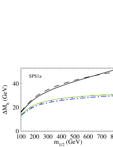
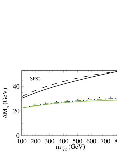
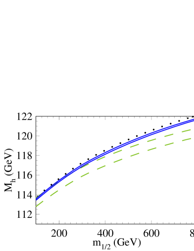
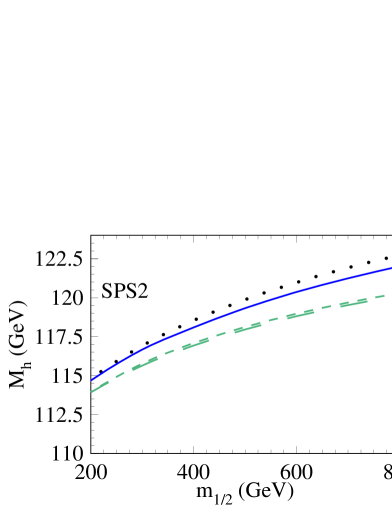
In the following we discuss the relative contribution to the Higgs boson mass comparing ΔMh(i)Δsuperscriptsubscript𝑀𝑖\Delta M_{h}^{(i)} and Δmt4Mh(i)superscriptΔsuperscriptsubscript𝑚𝑡4superscriptsubscript𝑀𝑖\Delta^{m_{t}^{4}}M_{h}^{(i)} at one- and two-loop order (i=1,2𝑖12i=1,2) where both the on-shell and DR¯¯DR\overline{\mbox{DR}} scheme for the mass parameters and the mixing angle are considered. For illustration we adopt the scenarios SPS1a and SPS2 and show the Higgs boson mass as a function of m1/2subscript𝑚12m_{1/2}.

Refer to caption Refer to caption
(a) (b)
Figure 2: Comparison of complete and approximate one- and two-loop corrections to the Higgs boson mass for SPS1a (a) and SPS2 (b). The solid (full result) and dashed lines (mt4superscriptsubscript𝑚𝑡4m_{t}^{4} approximation) represent the results in the on-shell scheme where the upper and lower curves correspond to the one- and two-loop results, respectively. The two-loop DR¯¯DR\overline{\mbox{DR}} results are shown as dash-dotted (full result) and dotted (mt4superscriptsubscript𝑚𝑡4m_{t}^{4} approximation) curves.

The solid lines in Fig. 2 show the results for ΔMh(i)Δsuperscriptsubscript𝑀𝑖\Delta M_{h}^{(i)} using on-shell parameters222For the on-shell renormalization of the mixing angle we adopt the convention of Ref. [27]. for the masses and θtsubscript𝜃𝑡\theta_{t} as it is provided by FeynHiggs. The dashed lines correspond to the mt4superscriptsubscript𝑚𝑡4m_{t}^{4} approximation (Δmt4Mh(i)superscriptΔsuperscriptsubscript𝑚𝑡4superscriptsubscript𝑀𝑖\Delta^{m_{t}^{4}}M_{h}^{(i)}) which can be found in Refs. [16, 27] and has been confirmed by us by an independent calculation. The panels (a) and (b) correspond to the SPS1a and SPS2 benchmark scenarios, respectively, where the input parameters have been generated with the help of SOFTSUSY [28]. The small differences of the solid and dashed lines333In the case of SPS1a the two-loop dashed line is almost on top of the solid one. demonstrate that the leading top quark mass term approximates the full result to a high accuracy. This statement is also true in the DR¯¯DR\overline{\mbox{DR}} scheme. The corresponding two-loop results are shown in Fig. 2 as dash-dotted and dotted curves where the former corresponds to the full and the latter to the approximate result.

It is well known that the perturbative series can exhibit a bad convergence behaviour in case it is parametrized in terms of the on-shell quark masses444For a typical example we refer to the electroweak ρ𝜌\rho parameter. Using the on-shell top quark mass the four-loop corrections [29, 30, 31] are larger by a factor 50 as compared to the MS¯¯MS\overline{\rm MS} scheme. which is due to intrinsically large contributions related to the infra-red behaviour of the theory. Thus, it is tempting to re-parametrize the results for the Higgs boson mass in terms of DR¯¯DR\overline{\mbox{DR}} parameters for the top quark mass, the masses of the SUSY particles and the top squark mixing angle. Since the corrections are dominated by Δmt4Mh(i)superscriptΔsuperscriptsubscript𝑚𝑡4superscriptsubscript𝑀𝑖\Delta^{m_{t}^{4}}M_{h}^{(i)} it is sufficient to consider only this term and take over ΔremMh(i)superscriptΔremsuperscriptsubscript𝑀𝑖\Delta^{\rm rem}M_{h}^{(i)} from the output of FeynHiggs. In the remainder of the paper we will refer to this renormalization scheme as DR¯¯DR\overline{\mbox{DR}} scheme although it contains a mixture of on-shell and DR¯¯DR\overline{\mbox{DR}} parameters. Let us mention already at this point that from outside this mixture does not pose any complication in the practical use since the spectrum generator produces both on-shell and DR¯¯DR\overline{\mbox{DR}} parameters which then serve as input for the evaluation of Mhsubscript𝑀M_{h}.

Further below we will discuss the scheme dependence of Mhsubscript𝑀M_{h} and indeed show that the loop corrections are in general smaller in the DR¯¯DR\overline{\mbox{DR}} scheme (cf. Fig. 8). Similar studies can also be found in the literature [15, 9].

The considerations of this subsection motivates the following procedure at three loops: It is certainly sufficient to consider only the approximation Δmt4Mh(3)superscriptΔsuperscriptsubscript𝑚𝑡4superscriptsubscript𝑀3\Delta^{m_{t}^{4}}M_{h}^{(3)} since the size of the remaining term is expected to be below 100 MeV. Furthermore, we adopt the DR¯¯DR\overline{\mbox{DR}} scheme since we expect that the perturbative series shows a better convergence behaviour. In addition the evaluation of the counterterms themselves is significantly simpler. Actually, most of them are already available in the literature and the computation of the remaining ones is quite straightforward as we discuss in Appendix A. We provide the analytical results for the two-loop renormalization constants of the top squark masses and mixing angle, that can be easily expanded for the mass hierarchies considered in this paper. The multiplicative DR¯¯DR\overline{\mbox{DR}} renormalization constants of the top quark and gluino mass are mass independent and therefore valid for all hierarchies.

2.4 Construction of approximations

Considering the many different mass parameters entering the formula for the Higgs boson mass an exact calculation of the three-loop corrections is currently not feasible. However, due to the various hierarchies among the particle masses it is promising to consider expansions in properly chosen small parameters. As a guideline for the latter we follow the SPS scenarios as defined in Refs. [20, 21].

In order to construct approximations covering all SPS cases it is sufficient to consider the following hierarchies among the SUSY masses555We decided to keep the nomenclature for the hierarchies as they are in our internal computations and documents. The non-continuous numeration results from the fact that for testing purposes we have computed further hierachies which, however, are not included in the program H3m (cf. Section 4).

(h3)h3\displaystyle({\rm h3}) mq~mt~1mt~2mg~,subscript𝑚~𝑞subscript𝑚subscript~𝑡1subscript𝑚subscript~𝑡2subscript𝑚~𝑔\displaystyle m_{\tilde{q}}\approx m_{\tilde{t}_{1}}\approx m_{\tilde{t}_{2}}\approx m_{\tilde{g}}\,,
(h4)h4\displaystyle({\rm h4}) mq~mt~1mt~2mg~,much-greater-thansubscript𝑚~𝑞subscript𝑚subscript~𝑡1subscript𝑚subscript~𝑡2subscript𝑚~𝑔\displaystyle m_{\tilde{q}}\gg m_{\tilde{t}_{1}}\approx m_{\tilde{t}_{2}}\approx m_{\tilde{g}}\,,
(h5)h5\displaystyle({\rm h5}) mq~mt~2mt~1mg~,much-greater-thansubscript𝑚~𝑞subscript𝑚subscript~𝑡2much-greater-thansubscript𝑚subscript~𝑡1subscript𝑚~𝑔\displaystyle m_{\tilde{q}}\gg m_{\tilde{t}_{2}}\gg m_{\tilde{t}_{1}}\approx m_{\tilde{g}}\,,
(h6)h6\displaystyle({\rm h6}) mq~mt~2mg~mt~1,much-greater-thansubscript𝑚~𝑞subscript𝑚subscript~𝑡2subscript𝑚~𝑔much-greater-thansubscript𝑚subscript~𝑡1\displaystyle m_{\tilde{q}}\gg m_{\tilde{t}_{2}}\approx m_{\tilde{g}}\gg m_{\tilde{t}_{1}}\,,
(h6b)h6b\displaystyle({\rm h6b}) mq~mt~2mg~mt~1,subscript𝑚~𝑞subscript𝑚subscript~𝑡2subscript𝑚~𝑔much-greater-thansubscript𝑚subscript~𝑡1\displaystyle m_{\tilde{q}}\approx m_{\tilde{t}_{2}}\approx m_{\tilde{g}}\gg m_{\tilde{t}_{1}}\,,
(h9)h9\displaystyle({\rm h9}) mq~mt~1mt~2mg~,subscript𝑚~𝑞subscript𝑚subscript~𝑡1subscript𝑚subscript~𝑡2much-greater-thansubscript𝑚~𝑔\displaystyle m_{\tilde{q}}\approx m_{\tilde{t}_{1}}\approx m_{\tilde{t}_{2}}\gg m_{\tilde{g}}\,, (21)

where in the case of “much-greater-than\gg” an asymptotic expansion in the corresponding hierarchy is performed. In the case of “\approx” a naive Taylor expansion in the difference of the particle masses is sufficient. Throughout this paper, q~~𝑞\tilde{q} denotes any squark other than t~~𝑡\tilde{t}, and we assume a common mass value mq~mq~1=mq~2subscript𝑚~𝑞subscript𝑚subscript~𝑞1subscript𝑚subscript~𝑞2m_{\tilde{q}}\equiv m_{\tilde{q}_{1}}=m_{\tilde{q}_{2}} for all of these “heavy squarks”.

In all hierarchies we assume that the SUSY masses are larger than the top quark mass and perform an asymptotic expansion in the corresponding ratio. In the numerical results discussed below we include for the various hierarchies the expansion terms as given in Tab. 1 where the following notation has been introduced

x12subscript𝑥12\displaystyle x_{12} =\displaystyle= mt~1mt~2,subscript𝑚subscript~𝑡1subscript𝑚subscript~𝑡2\displaystyle\frac{m_{\tilde{t}_{1}}}{m_{\tilde{t}_{2}}}\,,
x2gsubscript𝑥2𝑔\displaystyle x_{2g} =\displaystyle= mt~2mg~,subscript𝑚subscript~𝑡2subscript𝑚~𝑔\displaystyle\frac{m_{\tilde{t}_{2}}}{m_{\tilde{g}}}\,,
x1gsubscript𝑥1𝑔\displaystyle x_{1g} =\displaystyle= x12x2g=mt~1mg~,subscript𝑥12subscript𝑥2𝑔subscript𝑚subscript~𝑡1subscript𝑚~𝑔\displaystyle x_{12}x_{2g}=\frac{m_{\tilde{t}_{1}}}{m_{\tilde{g}}}\,,
x1qsubscript𝑥1𝑞\displaystyle x_{1q} =\displaystyle= mt~1mq~,subscript𝑚subscript~𝑡1subscript𝑚~𝑞\displaystyle\frac{m_{\tilde{t}_{1}}}{m_{\tilde{q}}}\,,
x2qsubscript𝑥2𝑞\displaystyle x_{2q} =\displaystyle= mt~2mq~.subscript𝑚subscript~𝑡2subscript𝑚~𝑞\displaystyle\frac{m_{\tilde{t}_{2}}}{m_{\tilde{q}}}\,. (22)
hierarchy expansion depth
(h3) (1x122)3superscript1superscriptsubscript𝑥1223(1-x_{12}^{2})^{3}, (1x1g)3superscript1subscript𝑥1𝑔3(1-x_{1g})^{3}, (1x1q2)3superscript1superscriptsubscript𝑥1𝑞23(1-x_{1q}^{2})^{3}
(h4) x1q8superscriptsubscript𝑥1𝑞8x_{1q}^{8}
(h5) (1x1g)2superscript1subscript𝑥1𝑔2(1-x_{1g})^{2}, (x12)4superscriptsubscript𝑥124(x_{12})^{4}, x2q4superscriptsubscript𝑥2𝑞4x_{2q}^{4}
(h6) x123superscriptsubscript𝑥123x_{12}^{3}, (1x2g)2superscript1subscript𝑥2𝑔2(1-x_{2g})^{2}, x2q4superscriptsubscript𝑥2𝑞4x_{2q}^{4}
(h6b) x123superscriptsubscript𝑥123x_{12}^{3}, (1x2g)2superscript1subscript𝑥2𝑔2(1-x_{2g})^{2}, (1x2q2)2superscript1superscriptsubscript𝑥2𝑞22(1-x_{2q}^{2})^{2}
(h9) (1x122)3superscript1superscriptsubscript𝑥1223(1-x_{12}^{2})^{3}, 1/x1241superscriptsubscript𝑥1241/x_{12}^{4}, (1x1q2)3superscript1superscriptsubscript𝑥1𝑞23(1-x_{1q}^{2})^{3}
Table 1: Expansion terms available for the individual hierarchies as defined in Eq. (21) at three-loop order.

Note that at two-loop order the contributions involving the squarks q~~𝑞\tilde{q} with q{u,d,s,c,b}𝑞𝑢𝑑𝑠𝑐𝑏q\in\{u,d,s,c,b\} cancel in the sum of all diagrams. At three-loop level, however, the results depend on mq~subscript𝑚~𝑞m_{\tilde{q}}. In those cases where mq~subscript𝑚~𝑞m_{\tilde{q}} is much larger than the other masses at least three expansion terms are computed and a good convergence even up to mq~mt~2subscript𝑚~𝑞subscript𝑚subscript~𝑡2m_{\tilde{q}}\approx m_{\tilde{t}_{2}} is observed.

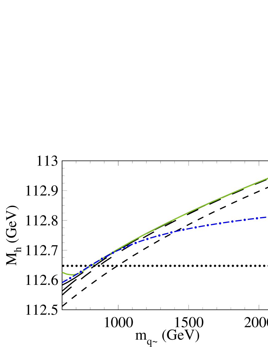
In order to demonstrate this point we consider the hierarchies (h3) and (h4) and show in Fig. 3 the three-loop prediction for Mhsubscript𝑀M_{h}. The dashed and solid lines correspond to (h4) including successively higher orders in 1/mq~1subscript𝑚~𝑞1/m_{\tilde{q}} where for illustration the following input parameters have been chosen:666If not stated otherwise we set the renormalization scale equal to the on-shell top quark mass and evaluate all DR¯¯DR\overline{\mbox{DR}} parameters at that scale. Note, however, that H3m is not restricted to this choice.

mSUSYsubscript𝑚SUSY\displaystyle m_{\rm SUSY} \displaystyle\equiv mg~=mt~1=mt~2=  800GeV,subscript𝑚~𝑔subscript𝑚subscript~𝑡1subscript𝑚subscript~𝑡2800GeV\displaystyle m_{\tilde{g}}\,\,=\,\,m_{\tilde{t}_{1}}\,\,=\,\,m_{\tilde{t}_{2}}\,\,=\,\,800\,\text{GeV}\,,
Atsubscript𝐴𝑡\displaystyle A_{t} =\displaystyle= μSUSY=θt=  0,subscript𝜇SUSYsubscript𝜃𝑡  0\displaystyle\mu_{\rm SUSY}\,\,=\,\,\theta_{t}\,\,=\,\,0\,,
MAsubscript𝑀𝐴\displaystyle M_{A} =\displaystyle= 1500GeV.1500GeV\displaystyle 1500~{}\mbox{GeV}\,. (23)

The horizontal (mq~subscript𝑚~𝑞m_{\tilde{q}}-independent) dotted line corresponds to the scenario (h3) with mq~=mSUSYsubscript𝑚~𝑞subscript𝑚SUSYm_{\tilde{q}}=m_{\rm SUSY} fixed at 800 GeV. One observes a crossing of the latter and the (h4)-curve including 1/mq~81superscriptsubscript𝑚~𝑞81/m_{\tilde{q}}^{8} corrections for mq~mSUSYsubscript𝑚~𝑞subscript𝑚SUSYm_{\tilde{q}}\approx m_{\rm SUSY} which nicely demonstrates the rapid convergence in the large-mq~subscript𝑚~𝑞m_{\tilde{q}} expansion. Fig. 3 also shows that the expansion around mq~=mSUSYsubscript𝑚~𝑞subscript𝑚SUSYm_{\tilde{q}}=m_{\rm SUSY} leads to good approximations even if mq~subscript𝑚~𝑞m_{\tilde{q}} is two to three times as big as mSUSYsubscript𝑚SUSYm_{\rm SUSY}, see dash-dotted curve. Note that for this plot we computed the DR¯¯DR\overline{\mbox{DR}} top quark mass for mq~=800subscript𝑚~𝑞800m_{\tilde{q}}=800 GeV and kept it fixed.

Refer to caption
Figure 3: Dependence of the three-loop corrections on the heavy squark mass mq~subscript𝑚~𝑞m_{\tilde{q}}. The dashed and solid lines correspond to the hierarchy (h4) where successively higher order terms in mSUSY/mq~subscript𝑚SUSYsubscript𝑚~𝑞m_{\rm SUSY}/m_{\tilde{q}} have been included (The solid curve contains terms of order (mSUSY2/mq~2)4superscriptsuperscriptsubscript𝑚SUSY2superscriptsubscript𝑚~𝑞24(m_{\rm SUSY}^{2}/m_{\tilde{q}}^{2})^{4}.). The dotted and dash-dotted curves correspond to the hierarchy (h3); for the dotted line mq~subscript𝑚~𝑞m_{\tilde{q}} has been kept fixed at 800 GeV, the dash-dotted curve includes terms of order (1mSUSY2/mq~2)3superscript1superscriptsubscript𝑚SUSY2superscriptsubscript𝑚~𝑞23(1-m_{\rm SUSY}^{2}/m_{\tilde{q}}^{2})^{3}.

Let us in a next step compare the approximate SQCD corrections according to our hierarchies with the full prediction for Mhsubscript𝑀M_{h} from Ref. [27]. For illustration we adopt in the remainder of this Section a minimal supergravity (msugra) scenario with

tanβ𝛽\displaystyle\tan\beta =\displaystyle= 10,10\displaystyle 10\,,
A0subscript𝐴0\displaystyle A_{0} =\displaystyle= 0,0\displaystyle 0\,,
μSUSYsubscript𝜇SUSY\displaystyle\mu_{\rm SUSY} >\displaystyle> 0,0\displaystyle 0\,, (24)

and vary m0subscript𝑚0m_{0} and m1/2subscript𝑚12m_{1/2} as follows

60GeV60GeV\displaystyle 60~{}\mbox{GeV} <m0<absentsubscript𝑚0absent\displaystyle<m_{0}< 1600GeV,1600GeV\displaystyle 1600~{}\mbox{GeV}\,,
100GeV100GeV\displaystyle 100~{}\mbox{GeV} <m1/2<absentsubscript𝑚12absent\displaystyle<m_{1/2}< 800GeV.800GeV\displaystyle 800~{}\mbox{GeV}\,. (25)

We have checked that very similar results are obtained for other choices of tanβ,A0𝛽subscript𝐴0\tan\beta,A_{0}, and sign(μSUSY)subscript𝜇SUSY(\mu_{\rm SUSY}). Thus, our conclusions are at least valid for all msugra SPS scenarios (cf. Appendix C).
Refer to caption Refer to caption
(a) (b)
Refer to caption Refer to caption
(c) (d)
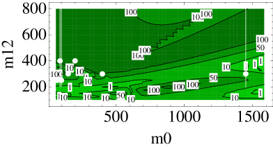
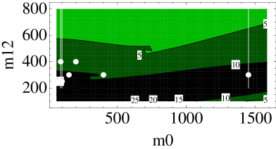
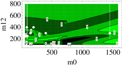
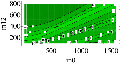
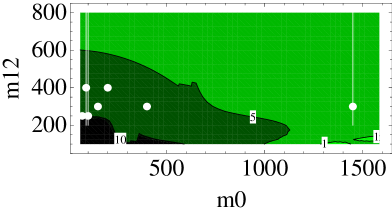
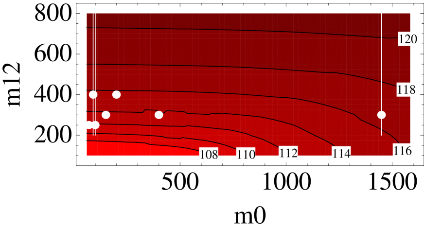
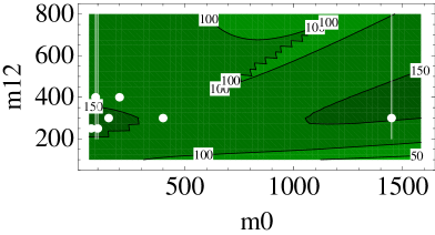
Figure 4: Comparison of approximate and full two-loop result for hierarchy (h3) (a) and the combination of (h3), (h5), (h6), (h6b) and (h9) (b). The contour lines indicate the deviations in MeV. In (c) and (d) the results of (a) and (b) are normalized to the genuine two-loop contributions where the contour lines indicate the deviations in per cent. The benchmark points and slopes are shown as (white) dots and lines.

In Fig. 4(a) and (b) the absolute value of the difference between the full and the approximate two-loop prediction for the Higgs boson mass, Mh(2)Mh(2),3lcutsuperscriptsubscript𝑀2superscriptsubscript𝑀23lcutM_{h}^{(2)}-M_{h}^{(2),\rm 3lcut}, is shown in the m0subscript𝑚0m_{0}-m1/2subscript𝑚12m_{1/2} plane where Mh(2),3lcutsuperscriptsubscript𝑀23lcutM_{h}^{(2),\rm{3lcut}} includes the same number of expansion terms which are available at three loops. In Fig. 4(a) we only include the results from hierarchy (h3) whereas in (b) also (h5), (h6), (h6b) and (h9) enter. For each hierarchy we compute the difference to the exact result and plot in Fig. 4(b) the minimum. We define the relative uncertainty through

δ(2)superscript𝛿2\displaystyle\delta^{(2)} =\displaystyle= Mh(2)Mh(2),3lcutMh(2)Mh(1),superscriptsubscript𝑀2superscriptsubscript𝑀23lcutsuperscriptsubscript𝑀2superscriptsubscript𝑀1\displaystyle\frac{M_{h}^{(2)}-M_{h}^{(2),\rm 3lcut}}{M_{h}^{(2)}-M_{h}^{(1)}}\,, (26)

which is shown in Fig. 4(c) and (d). In Eq. (26) Mh(i)superscriptsubscript𝑀𝑖M_{h}^{(i)} corresponds to the exact i𝑖i-loop prediction. For reference we show in Fig. 4 the msugra SPS benchmark points and slopes as (white) dots and lines, having in mind that for some of them the values of tanβ𝛽\tan\beta and A0subscript𝐴0A_{0} are different from the ones chosen in Eq. (24). The assignment of the individual scenarios to the corresponding dot is easily done with the help of the table in Appendix C.

Already for (h3) alone one observes a good coverage in the whole m0subscript𝑚0m_{0}-m1/2subscript𝑚12m_{1/2} plane with deviations smaller than 150 MeV. This gets further improved after including the other hierarchies. For lower values of m1/2subscript𝑚12m_{1/2} one has relative deviations also above 10%, however, the absolute difference between the full result and the approximation is below 100 MeV.

In Tab. 2 we directly compare the two-loop predictions for Mhsubscript𝑀M_{h} for the benchmark points listed in the table in Appendix C and SPS7 and SPS8 (gauge-mediated supersymmetry breaking) [20]. As before, the full results are based on FeynHiggs and Ref. [27], and for Mh(2),apprsuperscriptsubscript𝑀2apprM_{h}^{(2),\rm appr} we use the approximation incorporated in H3m. An impressive agreement is found, often even below 100 MeV.

Mh(2)superscriptsubscript𝑀2M_{h}^{(2)} Mh(2),apprsuperscriptsubscript𝑀2apprM_{h}^{(2),\rm appr} optimal
(GeV) (GeV) hierarchy
SPS1a 111.81 111.84 h6b
SPS1a 113.26 113.27 h6b
SPS1b 115.53 115.64 h3
SPS2 115.65 115.77 h5
SPS3 114.63 114.77 h3
SPS4 113.73 113.77 h6
SPS5 111.66 111.83 h3
SPS7 112.20 112.21 h3
SPS8 114.19 114.20 h3
Table 2: Comparison of full and approximate two-loop prediction for Mhsubscript𝑀M_{h} for the different benchmark points.

The results discussed in this Subsection are very promising in view of the three-loop approximation. At two-loop order the expansion terms specified in Tab. 1 provide an excellent approximation to the full result. Thus, it can be assumed that the corresponding terms at three loops approximate the unknown result with high precision.

3 Technical details to the three-loop calculation

The three-loop calculation of the individual Green’s functions contributing to Mhsubscript𝑀M_{h} is organized as follows: All Feynman diagrams are generated with QGRAF [32]. In order to properly take into account the Majorana character of the gluino, the output is subsequently manipulated by a PERL script [33] which applies the rules given in Ref. [34]. The various diagram topologies are identified and transformed to FORM [35] with the help of q2e and exp [36, 37]. The program exp is also used in order to apply the asymptotic expansion (see, e.g., Ref. [38]) in the various mass hierarchies. The actual evaluation of the integrals is performed with the package MATAD [39], resulting in an expansion in d4𝑑4d-4 for each diagram, where d𝑑d is the space-time dimension.

The total number of three-loop diagrams amounts to 6706 and 7670 for the ϕ1subscriptitalic-ϕ1\phi_{1} and ϕ2subscriptitalic-ϕ2\phi_{2} self energies, respectively, and 845 and 982 for the corresponding tadpole contributions. The computation of the off-diagonal matrix element Σϕ12subscriptΣsubscriptitalic-ϕ12\Sigma_{\phi_{12}} involves 6136 diagrams, and the propagator of the pseudoscalar Higgs another 7670. The application of the asymptotic expansion significantly enlarges these numbers leading to about 37 000 (for (h3)) or even 94 000 (for (h6)) subdiagrams. Note that there are diagrams where, depending on the hierarchy, up to 15 subdiagrams have to be considered. A typical example is shown in Fig. 1(a).

A subtlety arises from diagrams as the one shown in Fig. 1(b). If both the external momentum and the ε𝜀\varepsilon-scalar mass are set to zero from the beginning, an infra-red divergence occurs and cancels the ultra-violet divergence of the integral. In effect, the diagram will be of order (d4)𝑑4(d-4) due to the ε𝜀\varepsilon-scalar algebra. In order to avoid this, we keep the external momentum q𝑞q non-zero, though much smaller than all other scales. The ultra-violet pole multiplied by the algebraic factor of (d4)𝑑4(d-4) then produces a finite contribution, while the infra-red divergence leads to (d4)ln(q2)𝑑4superscript𝑞2(d-4)\ln(q^{2}) and vanishes as d4𝑑4d\to 4.

Instead of the requirement q0𝑞0q\not=0 one could also introduce a nonzero mass for the ε𝜀\varepsilon-scalars in order to regulate the infra-red divergences. In the final result we again observe that the regulator is multiplied by an additional factor (d4)𝑑4(d-4) leading to a finite result for Mε0subscript𝑀𝜀0M_{\varepsilon}\to 0. We have checked that the latter prescription leads to identical results as the one with q0𝑞0q\not=0.

We refrain from presenting all available analytical results for the expansion in the various regions. They are implemented in the program H3m and thus easily accessible if necessary. However, for the convenience of the reader we provide in this Section the result for (h4), see Eq. (21), which could be useful for other applications. We will present the results expressed in terms of the DR¯¯DR\overline{\mbox{DR}} parameters αssubscript𝛼𝑠\alpha_{s}, mtsubscript𝑚𝑡m_{t}, mt~1subscript𝑚subscript~𝑡1m_{\tilde{t}_{1}}, mt~2subscript𝑚subscript~𝑡2m_{\tilde{t}_{2}}, mg~subscript𝑚~𝑔m_{\tilde{g}} and θtsubscript𝜃𝑡\theta_{t}. The corresponding counterterms can be found in Appendix A.

Before providing explicit expressions a comment concerning the DR¯¯DR\overline{\mbox{DR}} renormalization constants for the top squarks is in order. Due to diagrams involving heavy squarks q~~𝑞\tilde{q}, for example Fig. 5(a), the squared Higgs boson mass receives contributions which are proportional to mq~2superscriptsubscript𝑚~𝑞2m_{\tilde{q}}^{2} and thus can lead to unnatural large corrections. For this reason we adopt the on-shell scheme for these contributions to δZmt~1𝛿subscript𝑍subscript𝑚subscript~𝑡1\delta Z_{{m}_{\tilde{t}_{1}}} and δZmt~2𝛿subscript𝑍subscript𝑚subscript~𝑡2\delta Z_{{m}_{\tilde{t}_{2}}} (cf. Eq. (65) and Fig. 5(b) for a sample diagram). This avoids the potentially large terms mq~2similar-toabsentsuperscriptsubscript𝑚~𝑞2\sim m_{\tilde{q}}^{2} from the three-loop diagrams. We follow this procedure also in the case where the top squarks and the “heavy squarks” are degenerate in mass. The renormalization of the mixing angle is free of such enhanced contributions and we can stick to the pure DR¯¯DR\overline{\mbox{DR}} scheme in that case. We hasten to add that this discussion only concerns the internal structure of H3m and has no direct consequences for the user. The input parameters of H3m are the DR¯¯DR\overline{\mbox{DR}} ones as they appear, e.g., in the output of SOFTSUSY.

As already noticed in Refs. [16, 27], a similar behaviour is observed when the gluino is much heavier than the top squarks. In this case, the two- and three-loop corrections to the Higgs masses computed in the DR¯¯DR\overline{\mbox{DR}} scheme contain terms proportional to mg~subscript𝑚~𝑔m_{\tilde{g}} and mg~2superscriptsubscript𝑚~𝑔2m_{\tilde{g}}^{2}. These contributions are canceled in the on-shell scheme by the finite parts of the relevant counterterms. Thus, in order to avoid unnatural large radiative corrections to the Higgs masses, we adopt for scenarios with heavy gluino masses a modified renormalization scheme for the top squark masses. We call this scheme “modified DR¯¯DR\overline{\mbox{DR}}” (MDR¯¯MDR\overline{\mbox{MDR}}) and it is characterized by the non minimal renormalization of the top squark masses. The additional finite shifts of top squark masses are chosen such that they cancel the power-like behaviour of the gluino contributions. Again, the renormalization of the mixing angle will not be modified as compared to the genuine DR¯¯DR\overline{\mbox{DR}} scheme.

The relevant finite shifts for the scenarios considered in this paper are explicitly given in Appendix B. As can be noticed from Eq. (21) the scenarios (h4), (h5) and (h6) display heavy squark mass contributions whereas heavy gluino terms are specific only for the scenarios (h6) and (h6b).

In the practical calculation we use the DR¯¯DR\overline{\mbox{DR}} top squark mass parameters as provided by the spectrum generators and transform them with the help of the formulae of Appendix B to the corresponding parameters in the MDR¯¯MDR\overline{\mbox{MDR}} scheme which constitute the input for our analytic expressions.

Refer to caption Refer to caption
(a) (b)
Figure 5: (a) Feynman diagram involving a heavy virtual squark contributing to the Higgs boson self energy. (b) Counterterm diagram related to the diagram in (a). The same notation as in Fig. 1 has been adopted.

In the following we present results for the renormalized two-point functions Σ^ϕ1subscript^Σsubscriptitalic-ϕ1\hat{\Sigma}_{\phi_{1}}, Σ^ϕ2subscript^Σsubscriptitalic-ϕ2\hat{\Sigma}_{\phi_{2}} and Σ^ϕ1ϕ2subscript^Σsubscriptitalic-ϕ1subscriptitalic-ϕ2\hat{\Sigma}_{\phi_{1}\phi_{2}} for the hierarchy (h4) which for equal top squark and gluino masses take the form777We only include terms up to order 1/mq~21superscriptsubscript𝑚~𝑞21/m_{\tilde{q}}^{2}.

Σ^ϕ2subscript^Σsubscriptitalic-ϕ2\displaystyle\hat{\Sigma}_{\phi_{2}} =GFmt42π2sin2β[32ltS+αs4π(4+(4+16lμt)ltS+4ltS2+AtmSUSY(4+8lμt+4ltS))\displaystyle=\frac{G_{F}m_{t}^{4}\sqrt{2}}{\pi^{2}\sin^{2}\beta}\bigg{[}\frac{3}{2}l_{tS}+\frac{\alpha_{s}}{4\pi}\bigg{(}4+\Big{(}4+16l_{{\mu}t}\Big{)}l_{tS}+4l_{tS}^{2}+\frac{A_{t}}{m_{\rm SUSY}}\Big{(}4+8l_{{\mu}t}+4l_{tS}\Big{)}\bigg{)}
+(αs4π)2{2764911627lμt1363lμt2+(6449+1643lμt)ltS2+24ltS3+4003ltq~2003ltq~2203ltq~3120ζ(2)80ltq~ζ(2)+83ζ(3)(221627+6449lμt3283lμt240ltq~20ltq~240ζ(2)+16ζ(3))ltS+mq~2mSUSY2(40+80lμt+80ltq~+80ζ(2))+mSUSY2mq~2(42356225+8ltS2212845ltq~1763ltq~2+(392845+1523ltq~)ltS4003ζ(2))+AtmSUSYmq~2(80+ltS(3209803ltq~)+3209ltq~+803ltq~2+1603ζ(2))+AtmSUSY(83227+72827lμt+2003lμt2+6089ltS2+ltS(125627+8009lμt1603ltq~)4009ltq~+40ltq~2+80ζ(2)2123ζ(3))+At2mSUSY2(3499+329lμt+329lμt2+(569+649lμt)ltS+329ltS2+943ζ(3))}+𝒪(mSUSY4mq~4)],\displaystyle+\left(\frac{\alpha_{s}}{4\pi}\right)^{\!2}\negthickspace\begin{aligned} \bigg{\{}{}&\frac{2764}{9}-\frac{116}{27}l_{{\mu}t}-\frac{136}{3}l_{{\mu}t}^{2}+\bigg{(}-\frac{644}{9}+\frac{164}{3}l_{{\mu}t}\bigg{)}l_{tS}^{2}\\ &+24l_{tS}^{3}+\frac{400}{3}l_{t\tilde{q}}-\frac{200}{3}l_{t\tilde{q}}^{2}-\frac{20}{3}l_{t\tilde{q}}^{3}-120\zeta({2})-80l_{t\tilde{q}}\zeta({2})+\frac{8}{3}\zeta({3})\\ &-\bigg{(}\frac{2216}{27}+\frac{644}{9}l_{{\mu}t}-\frac{328}{3}l_{{\mu}t}^{2}-40l_{t\tilde{q}}-20l_{t\tilde{q}}^{2}-40\zeta({2})+16\zeta({3})\bigg{)}l_{tS}\\ &+\frac{m_{\tilde{q}}^{2}}{m_{\rm SUSY}^{2}}\bigg{(}-40+80l_{{\mu}t}+80l_{t\tilde{q}}+80\zeta({2})\biggr{)}\\ &+\frac{m_{\rm SUSY}^{2}}{m_{\tilde{q}}^{2}}\begin{aligned} \bigg{(}{}&\frac{42356}{225}+8l_{tS}^{2}-\frac{2128}{45}l_{t\tilde{q}}-\frac{176}{3}l_{t\tilde{q}}^{2}\\ &+\Big{(}\frac{3928}{45}+\frac{152}{3}l_{t\tilde{q}}\Big{)}l_{tS}-\frac{400}{3}\zeta({2})\bigg{)}\end{aligned}\\ &+\frac{A_{t}m_{\rm SUSY}}{m_{\tilde{q}}^{2}}\begin{aligned} \bigg{(}{}&-80+l_{tS}\Big{(}-\frac{320}{9}-\frac{80}{3}l_{t\tilde{q}}\Big{)}+\frac{320}{9}l_{t\tilde{q}}+\frac{80}{3}l_{t\tilde{q}}^{2}+\frac{160}{3}\zeta({2})\bigg{)}\end{aligned}\\ &+\frac{A_{t}}{m_{\rm SUSY}}\begin{aligned} \bigg{(}{}&\frac{832}{27}+\frac{728}{27}l_{{\mu}t}+\frac{200}{3}l_{{\mu}t}^{2}+\frac{608}{9}l_{tS}^{2}\\ &+l_{tS}\Big{(}\frac{1256}{27}+\frac{800}{9}l_{{\mu}t}-\frac{160}{3}l_{t\tilde{q}}\Big{)}\\ &-\frac{400}{9}l_{t\tilde{q}}+40l_{t\tilde{q}}^{2}+80\zeta({2})-\frac{212}{3}\zeta({3})\bigg{)}\end{aligned}\\ &+\frac{A_{t}^{2}}{m_{\rm SUSY}^{2}}\begin{aligned} \bigg{(}{}&-\frac{349}{9}+\frac{32}{9}l_{{\mu}t}+\frac{32}{9}l_{{\mu}t}^{2}+\Big{(}\frac{56}{9}+\frac{64}{9}l_{{\mu}t}\Big{)}l_{tS}\\ &+\frac{32}{9}l_{tS}^{2}+\frac{94}{3}\zeta({3})\bigg{)}\bigg{\}}+\mathcal{O}\left(\frac{m_{\rm SUSY}^{4}}{m_{\tilde{q}}^{4}}\right)\bigg{]}\,,\end{aligned}\end{aligned}
Σ^ϕ1subscript^Σsubscriptitalic-ϕ1\displaystyle\hat{\Sigma}_{\phi_{1}} =GFmt42π2cos2β(αs4π)2At2mSUSY2[3499+329lμt+329lμt2+(569+649lμt)ltS+329ltS2+943ζ(3)+𝒪(mSUSY4mq~4)],\displaystyle=\frac{G_{F}m_{t}^{4}\sqrt{2}}{\pi^{2}\cos^{2}\beta}\begin{aligned} \left(\frac{\alpha_{s}}{4\pi}\right)^{\!2}&\frac{A_{t}^{2}}{m_{\rm SUSY}^{2}}\bigg{[}-\frac{349}{9}+\frac{32}{9}l_{{\mu}t}+\frac{32}{9}l_{{\mu}t}^{2}\\ &+\bigg{(}\frac{56}{9}+\frac{64}{9}l_{{\mu}t}\bigg{)}l_{tS}+\frac{32}{9}l_{tS}^{2}+\frac{94}{3}\zeta({3})+\mathcal{O}\left(\frac{m_{\rm SUSY}^{4}}{m_{\tilde{q}}^{4}}\right)\bigg{]}\,,\end{aligned}
Σ^ϕ12subscript^Σsubscriptitalic-ϕ12\displaystyle\hat{\Sigma}_{\phi_{12}} =GFmt42π2cosβsinβ[αs4πAtmSUSY(24lμt2ltS)\displaystyle=\frac{G_{F}m_{t}^{4}\sqrt{2}}{\pi^{2}\cos\beta\sin\beta}\bigg{[}\frac{\alpha_{s}}{4\pi}\frac{A_{t}}{m_{\rm SUSY}}\Big{(}-2-4l_{{\mu}t}-2l_{tS}\Big{)}
+(αs4π)2{At2mSUSY2(3499329lμt329lμt2+(569649lμt)ltS329ltS2943ζ(3))+AtmSUSYmq~2(401609ltq~403ltq~2+ltS(1609+403ltq~)803ζ(2))+AtmSUSY(4162736427lμt1003lμt23049ltS2+2009ltq~20ltq~2+ltS(628274009lμt+803ltq~)40ζ(2)+1063ζ(3))}+𝒪(mSUSY4mq~4)],\displaystyle+\left(\frac{\alpha_{s}}{4\pi}\right)^{\!2}\negthickspace\begin{aligned} \bigg{\{}{}&\frac{A_{t}^{2}}{m_{\rm SUSY}^{2}}\begin{aligned} \bigg{(}{}&\frac{349}{9}-\frac{32}{9}l_{{\mu}t}-\frac{32}{9}l_{{\mu}t}^{2}+\Big{(}-\frac{56}{9}-\frac{64}{9}l_{{\mu}t}\Big{)}l_{tS}-\frac{32}{9}l_{tS}^{2}-\frac{94}{3}\zeta({3})\bigg{)}\end{aligned}\\ &+\frac{A_{t}m_{\rm SUSY}}{m_{\tilde{q}}^{2}}\bigg{(}40-\frac{160}{9}l_{t\tilde{q}}-\frac{40}{3}l_{t\tilde{q}}^{2}+l_{tS}\Big{(}\frac{160}{9}+\frac{40}{3}l_{t\tilde{q}}\Big{)}-\frac{80}{3}\zeta({2})\bigg{)}\\ &+\frac{A_{t}}{m_{\rm SUSY}}\bigg{(}-\frac{416}{27}-\frac{364}{27}l_{{\mu}t}-\frac{100}{3}l_{{\mu}t}^{2}-\frac{304}{9}l_{tS}^{2}+\frac{200}{9}l_{t\tilde{q}}-20l_{t\tilde{q}}^{2}\\ &+l_{tS}\Big{(}-\frac{628}{27}-\frac{400}{9}l_{{\mu}t}+\frac{80}{3}l_{t\tilde{q}}\Big{)}-40\zeta({2})+\frac{106}{3}\zeta({3})\bigg{)}\bigg{\}}+\mathcal{O}\left(\frac{m_{\rm SUSY}^{4}}{m_{\tilde{q}}^{4}}\right)\bigg{]}\,,\end{aligned}

with mt=mt(μr)subscript𝑚𝑡subscript𝑚𝑡subscript𝜇𝑟m_{t}=m_{t}(\mu_{r}), mSUSY=mSUSY(μr)=mt~1(μr)=mt~2(μr)=mg~(μr)subscript𝑚SUSYsubscript𝑚SUSYsubscript𝜇𝑟subscript𝑚subscript~𝑡1subscript𝜇𝑟subscript𝑚subscript~𝑡2subscript𝜇𝑟subscript𝑚~𝑔subscript𝜇𝑟m_{\rm SUSY}=m_{\rm SUSY}(\mu_{r})=m_{\tilde{t}_{1}}(\mu_{r})=m_{\tilde{t}_{2}}(\mu_{r})=m_{\tilde{g}}(\mu_{r}), lμt=ln(μr2/mt2)subscript𝑙𝜇𝑡superscriptsubscript𝜇𝑟2superscriptsubscript𝑚𝑡2l_{{\mu}t}=\ln(\mu_{r}^{2}/m_{t}^{2}), ltS=ln(mt2/mSUSY2)subscript𝑙𝑡𝑆superscriptsubscript𝑚𝑡2superscriptsubscript𝑚SUSY2l_{tS}=\ln(m_{t}^{2}/m_{\rm SUSY}^{2}) and ltq~=ln(mt2/mq~2)subscript𝑙𝑡~𝑞superscriptsubscript𝑚𝑡2superscriptsubscript𝑚~𝑞2l_{t\tilde{q}}=\ln(m_{t}^{2}/m_{\tilde{q}}^{2}) where μrsubscript𝜇𝑟\mu_{r} is the renormalization scale. The on-shell result corresponding to Σ^ϕ2subscript^Σsubscriptitalic-ϕ2\hat{\Sigma}_{\phi_{2}} has been presented in Ref. [13] for At=0subscript𝐴𝑡0A_{t}=0.

We refrain from providing more analytic results since all of them come along with the program H3m which is discussed in the next section.

4 Description of H3m

In this Section we describe the implementation of our three-loop results in a user-friendly computer program which allows the evaluation of the light CP even Higgs boson mass Mhsubscript𝑀M_{h} to three-loop accuracy. The program is implemented in the form of a Mathematica package.

To set the input parameters for the calculation, i.e. the SUSY spectrum and SM parameters, the SUSY Les Houches Accord (slha[40] is used. For ease of use, we provide functions that call a spectrum generator from Mathematica to produce an slha spectrum file. To produce the plots in this publication, we have chosen SOFTSUSY [28], but it is possible to use any spectrum generator that provides the DR¯¯DR\overline{\mbox{DR}} parameters in addition to the on-shell mass spectrum like SuSpect [41] or SPheno [42]. The advantage of SOFTSUSY is that the renormalization scale of the DR¯¯DR\overline{\mbox{DR}} parameters can be chosen independently of the electroweak symmetry breaking.

The corrections Δmt4MhsuperscriptΔsuperscriptsubscript𝑚𝑡4subscript𝑀\Delta^{m_{t}^{4}}M_{h} to Mhsubscript𝑀M_{h}, being proportional to the fourth power of the mass of the top quark mtsubscript𝑚𝑡m_{t}, are very sensitive to both the definition and the uncertainty of mtsubscript𝑚𝑡m_{t}. Thus, it is important to use the most precise value of mtsubscript𝑚𝑡m_{t} available. For this reason we take into account the full two-loop SQCD corrections between the on-shell and DR¯¯DR\overline{\mbox{DR}} top quark mass given in Ref. [43].888We thank Steven Martin for providing us with the relevant formulae from Ref. [43] in electronic form, and for allowing us to include his code in our program. In this paper, the relation of the on-shell top mass Mtsubscript𝑀𝑡M_{t} and DR¯¯DR\overline{\mbox{DR}} top mass mtsubscript𝑚𝑡m_{t} was derived as a function of the DR¯¯DR\overline{\mbox{DR}} masses. Solving this equation iteratively, we get mtsubscript𝑚𝑡m_{t} as a function of Mtsubscript𝑀𝑡M_{t}. The integrals appearing in [43] are evaluated using the C library TSIL [44]. This relation is available for general renormalization scale μrsubscript𝜇𝑟\mu_{r} which enables us to obtain mt(μr)subscript𝑚𝑡subscript𝜇𝑟m_{t}(\mu_{r}) in the DR¯¯DR\overline{\mbox{DR}} scheme using the on-shell mass Mtsubscript𝑀𝑡M_{t} as measured at the Tevatron [45] as input.

Another critical parameter for the evaluation of Mhsubscript𝑀M_{h} is the strong coupling αssubscript𝛼𝑠\alpha_{s}. We use αs(MZ)subscript𝛼𝑠subscript𝑀𝑍\alpha_{s}(M_{Z}) as input and follow Ref. [46, 47, 48] in order to evaluate αssubscript𝛼𝑠\alpha_{s} in the DR¯¯DR\overline{\mbox{DR}} scheme with all SUSY particles contributing to the running. First, αs(5),MS¯(MZ)=0.1184superscriptsubscript𝛼𝑠5¯MSsubscript𝑀𝑍0.1184\alpha_{s}^{(5),\overline{\rm MS}}(M_{Z})=0.1184 [49] is run up to the decoupling scale, which we set to the average value of the SUSY particles, using the four-loop β𝛽\beta function [50, 51]. There, we perform the transition to the DR¯¯DR\overline{\mbox{DR}} scheme and the full theory. The two-loop matching coefficients from [48] are used in this step. To obtain αs(full),DR¯(μr)superscriptsubscript𝛼𝑠full¯DRsubscript𝜇𝑟\alpha_{s}^{\rm(full),\overline{\rm DR}}(\mu_{r}) for arbitrary values of the renormalization scale μrsubscript𝜇𝑟\mu_{r}, we use the three-loop SQCD β𝛽\beta function given in [52, 33].

The remaining input parameters comprise the ones for the SUSY breaking scenario, which we summarise in the table of Appendix C and the SM parameters MZsubscript𝑀𝑍M_{Z}, GFsubscript𝐺𝐹G_{F} and α𝛼\alpha which also serve as input for the spectrum. The default values set in H3m read

MZsubscript𝑀𝑍\displaystyle M_{Z} =\displaystyle= 91.1876GeV,91.1876GeV\displaystyle 91.1876~{}\mbox{GeV}\,,
Mtsubscript𝑀𝑡\displaystyle M_{t} =\displaystyle= 173.1GeV,173.1GeV\displaystyle 173.1~{}\mbox{GeV}\,,
GFsubscript𝐺𝐹\displaystyle G_{F} =\displaystyle= 1.16637105GeV2,1.16637superscript105superscriptGeV2\displaystyle 1.16637\cdot 10^{-5}~{}\mbox{GeV}^{-2}\,,
1/α(MZ)1𝛼subscript𝑀𝑍\displaystyle 1/\alpha(M_{Z}) =\displaystyle= 127.934,127.934\displaystyle 127.934\,,
αs(MZ)subscript𝛼𝑠subscript𝑀𝑍\displaystyle\alpha_{s}(M_{Z}) =\displaystyle= αs(5),MS¯(MZ)=  0.1184.superscriptsubscript𝛼𝑠5¯MSsubscript𝑀𝑍0.1184\displaystyle\alpha_{s}^{(5),\overline{\rm MS}}(M_{Z})\,\,=\,\,0.1184\,. (27)

Of course, it is possible to modify these default values. Note that the top squark masses and mixing angle are obtained from the soft breaking parameters according to Eqs. (13) and (19).

In order to include all the known corrections to Mhsubscript𝑀M_{h} at the one- and two-loop level, the spectrum file is passed to FeynHiggs [10, 14, 15, 16]. FeynHiggs uses on-shell parameters that are given in the spectrum file and provides the neutral Higgs mass matrix up to the two-loop level. Since we prefer to use the DR¯¯DR\overline{\mbox{DR}} scheme, we need to perform a conversion before adding our three-loop results. This we do by subtracting the on-shell expression for Δmt4MhsuperscriptΔsuperscriptsubscript𝑚𝑡4subscript𝑀\Delta^{m_{t}^{4}}M_{h} (up to two loops, without any expansions in the masses999We thank Pietro Slavich for sending us the compact formulae from Ref. [27] in electronic form.) and adding it back in the DR¯¯DR\overline{\mbox{DR}} scheme. Thus, we use the DR¯¯DR\overline{\mbox{DR}} scheme to evaluate Δmt4MhsuperscriptΔsuperscriptsubscript𝑚𝑡4subscript𝑀\Delta^{m_{t}^{4}}M_{h}, which are dominant and sensitive to the top quark mass, and the on-shell scheme for ΔremMhsuperscriptΔremsubscript𝑀\Delta^{\rm rem}M_{h}.

The next step is to choose a suitable mass hierarchy for the expansion of the three-loop corrections. This is done by comparing, at the two-loop level, the full result from Ref. [27] with the expansions in all the mass hierarchies and choosing the one minimizing the error. Finally, the three-loop corrections are added, the neutral Higgs mass matrix is diagonalized, and the mass of the light Higgs is returned to the user.

Refer to caption
Figure 6: Flowchart of H3m. First, the user calls H3SetSLHA or one of its descendants to set the parameters. A subsequent call to H3mcomputes Mhsubscript𝑀M_{h}.

The interface of the program is outlined in Fig. 6. The parameters are set up by a call of the function H3SetSLHA, which passes its arguments to the spectrum generator and parses its output to get the relevant input parameters for the calculation. The top mass and strong coupling are calculated as described above. Alternatively, the function H3GetSLHA uses an existing spectrum file instead of running a generator. For the user interested in the Snowmass Points and Slopes, we provide convenient wrapper functions H3SetSPS<x> which call H3SetSLHA with parameters according to a specific benchmark scenario.

The main calculation is organized by the function H3m, which calls FeynHiggs, does the conversion to the DR¯¯DR\overline{\mbox{DR}} scheme described above, chooses an appropriate mass hierarchy, adds the three-loop corrections, and returns Mhsubscript𝑀M_{h}.

In Fig. 7, a typical Mathematica session with H3m is shown. A more detailed description of H3m comes along with the program which can be found at the web page [22].

Mathematica 7.0 for Linux x86 (64-bit)
Copyright 1988-2008 Wolfram Research, Inc.

In[1]:= Needs["H3‘"];

RunDec: a Mathematica package for running and decoupling of the
        strong coupling and quark masses
by K.G. Chetyrkin, J.H. Kuhn and M. Steinhauser (January 2000)

In[2]:= H3SetSPS1a[ 300.];

H3GetSLHA::TSIL: Using TSIL by S.P. Martin.
 -----------------------------------------------------
 FeynHiggs 2.6.5
 built on Dec 20, 2008
 T. Hahn, S. Heinemeyer, W. Hollik, H. Rzehak, G. Weiglein
 http://www.feynhiggs.de
 -----------------------------------------------------
 FHHiggsCorr contains code by:
 P. Slavich et al. (2-loop rMSSM Higgs self-energies)
Loading Results for hierarchy h3
Loading Results for hierarchy h6b2qg2

In[3]:= H3m[]

Loading Results for hierarchy h6b2qg2

Out[3]= {mh -> 114.176}
Figure 7: A typical Mathematica session with H3m.

5 The Higgs boson mass to three-loop accuracy

In this Section we use, if not stated otherwise, the input parameters as listed in Eq. (27) and furthermore adopt for the renormalization scale μr=Mtsubscript𝜇𝑟subscript𝑀𝑡\mu_{r}=M_{t} as our default value.

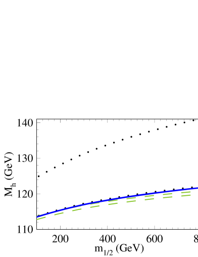
In Fig. 8 we show the renormalization scheme dependence of Mhsubscript𝑀M_{h} as a function of m1/2subscript𝑚12m_{1/2} for the SPS2 scenario. This is convenient since we have the same abscissa both for the on-shell and DR¯¯DR\overline{\mbox{DR}} result. Note, however, that the three-loop on-shell result is only available for a degenerate mass spectrum of the SUSY particles and vanishing parameter Atsubscript𝐴𝑡A_{t} [13]. Thus, we restrict ourselves to this limit also for the DR¯¯DR\overline{\mbox{DR}} result. For this reason the following discussion should be considered in a less quantitative but more qualitative sense and should not be used, e.g., for estimating a theoretical uncertainty.

In the left panel of Fig. 8 the upper dotted, dashed and solid curve correspond to the one-, two- and three-loop prediction of Mhsubscript𝑀M_{h} in the on-shell scheme whereas the corresponding lower three curves are obtained in the DR¯¯DR\overline{\mbox{DR}} scheme. In the on-shell scheme one observes large positive one-loop corrections which get reduced by 10 to 20 GeV after including the two-loop terms. The three-loop corrections amount to several hundred MeV. They are positive or negative — depending on the value of m1/2subscript𝑚12m_{1/2}.

The situation is completely different for DR¯¯DR\overline{\mbox{DR}} mass parameters: the one-loop corrections are significantly smaller and lead to values of Mhsubscript𝑀M_{h} which are already of the order of the two- and three-loop on-shell prediction. The two-loop term leads to a small shift of the order of 11-1 GeV and the three-loop term to a positive shift of about the same order of magnitude. The final prediction for Mhsubscript𝑀M_{h} is very close to the one obtained after incorporating three-loop on-shell results.101010The relatively large three-loop corrections (as compared to the two-loop ones) do not pose any problem since we use simplified formulae as mentioned before. Furthermore, there are regions in the parameter space where the two-loop corrections are accidentally small in the DR¯¯DR\overline{\mbox{DR}} scheme leading to large relative three-loop terms. Nevertheless the overall size of the two- and three-loop corrections is small.

Comparing the DR¯¯DR\overline{\mbox{DR}} and on-shell results in Fig. 8 one observes a nice reduction of the scheme dependence when incorporating higher order corrections.111111Up to two-loop order the scheme dependence has already been discussed in Fig. 2. Whereas there is a huge gap between the two one-loop curves (dotted) the difference in the two-loop prediction of Mhsubscript𝑀M_{h} is below 2 GeV which gets further reduced by about a factor ten after incorporating the three-loop corrections to roughly 200 MeV.
Refer to caption Refer to caption
Figure 8: Renormalization scheme dependence of Mhsubscript𝑀M_{h} as a function of m1/2subscript𝑚12m_{1/2} adopting SPS2. Dotted, dashed and solid curves correspond to one-, two- and three-loop results. The DR¯¯DR\overline{\mbox{DR}} (on-shell) results correspond to the lower (upper) three curves. In the right panel the interesting part of the left one is magnified.
Refer to caption Refer to caption
(a) (b)
Refer to caption Refer to caption
(c) (d)
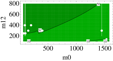
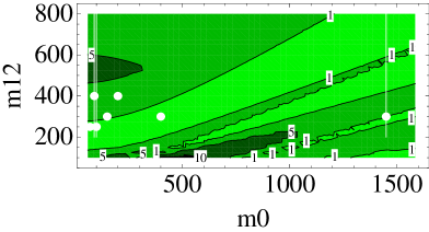
Figure 9: Comparison of the three-loop predictions for Mhsubscript𝑀M_{h} using the maximal available expansion terms and reduced input as described in the text. In (a) and (b) the absolute deviations are shown for the hierarchy (h3) and the combination of (h3), (h5), (h6), (h6b) and (h9), respectively. The contour lines indicate the deviations in MeV. In (c) and (d) the results of (a) and (b) are normalized to the genuine three-loop contributions where the contour lines indicate the deviations in per cent. The benchmark points and slopes are shown as (white) dots and lines.

Fig. 9 extends Fig. 4 to three loops. In (a) and (b) we again discuss the hierarchy (h3) and the combination of the hierarchies (h3), (h5), (h6), (h6b) and (h9), respectively, and show the difference between our best prediction and the one where the expansion parameters are cut by one unit.121212 We only cut in parameters originating from asymptotic expansion: when counting powers of mass ratios, we leave sin2θt2subscript𝜃𝑡\sin 2\theta_{t} untouched and do not replace it by Eq. (19). In the whole parameter plane we observe small absolute corrections reaching at most about 100 MeV. This leads to the conclusion that as a conservative estimate of the uncertainty of our approximation procedure one can assign about 100 MeV.

In Fig. 9(c) and (d) we show relative deviations defined through

δ(3)superscript𝛿3\displaystyle\delta^{(3)} =\displaystyle= Mh(3)Mh(3),cutMh(3)Mh(2),superscriptsubscript𝑀3superscriptsubscript𝑀3cutsuperscriptsubscript𝑀3superscriptsubscript𝑀2\displaystyle\frac{M_{h}^{(3)}-M_{h}^{(3),\rm cut}}{M_{h}^{(3)}-M_{h}^{(2)}}\,, (28)

where Mh(3)superscriptsubscript𝑀3M_{h}^{(3)} is our best three-loop prediction, Mh(3),cutsuperscriptsubscript𝑀3cutM_{h}^{(3),\rm cut} is the prediction where at three-loop order the expansion depth of each parameter (cf. Tab. 1) is reduced by one unit, and Mh(2)superscriptsubscript𝑀2M_{h}^{(2)} corresponds to the (full) two-loop term. Similar to the two-loop case, larger corrections are only observed for small values of m0subscript𝑚0m_{0} and m1/2subscript𝑚12m_{1/2} which is a consequence of a small denominator in Eq. (28). The three-loop correction terms, however, are stable as can be seen from the panels (a) and (b). Thus, as in the two-loop case, we are able to cover the whole m0subscript𝑚0m_{0}-m1/2subscript𝑚12m_{1/2} plane and are in particular able to produce precise values for Mhsubscript𝑀M_{h} for all SPS scenarios.

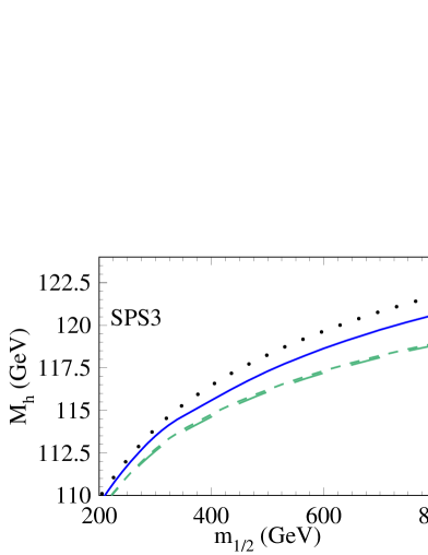
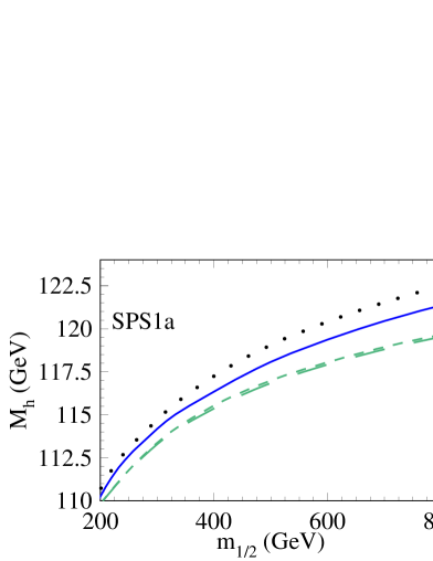
The slopes for three SPS scenarios are shown in Fig. 10(a), (b) and (c) where the dotted, dashed and solid lines correspond to the one-, two- and three-loop predictions, respectively. For all three cases one observes negative corrections between 1 and 4 GeV at two loops and positive contributions from the three-loop term which amount up to about 2 GeV.
Refer to caption Refer to caption
(a) (b)
Refer to caption Refer to caption
(c) (d)
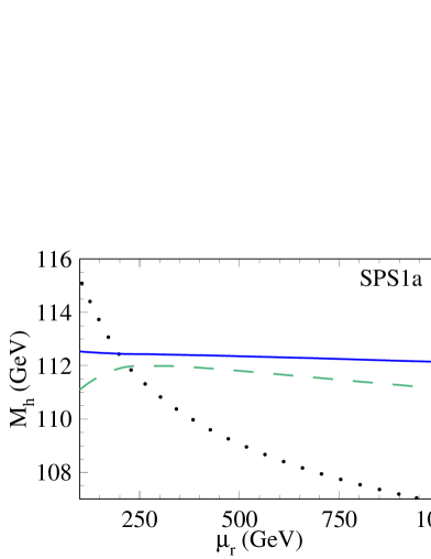
Figure 10: Mhsubscript𝑀M_{h} for the different slopes of the benchmark scenarios SPS1a (a), SPS2 (b) and SPS3 (c). Dotted, dashed and solid lines correspond to the one-, two- and three-loop predictions. The dashed line with longer dashes (at two loops) correspond to the full results, the one with the shorter dashes to the approximation implemented in H3m. In (d) the dependence of Mhsubscript𝑀M_{h} on the renormalization scale is shown where the dotted, dashed and solid line corresponds to the one-, two- and three-loop prediction.

In Fig. 10(d) we show the dependence of the prediction for Mhsubscript𝑀M_{h} on the renormalization scale μrsubscript𝜇𝑟\mu_{r}. As an example we adopt the SPS1a scenario with m1/2=250subscript𝑚12250m_{1/2}=250 GeV and exploit that SOFTSUSY allows the evaluation of all DR¯¯DR\overline{\mbox{DR}} parameters at the scale μrsubscript𝜇𝑟\mu_{r}. One observes a strong dependence at one-loop order which gets significantly reduced at two loops. The three-loop curve is even more flat resulting in a stable prediction for Mhsubscript𝑀M_{h}. Around μr=250subscript𝜇𝑟250\mu_{r}=250 GeV the two-loop correction shows a local maximum and is furthermore very small whereas the three-loop term still amounts to about 500 MeV. Around μr=Mtsubscript𝜇𝑟subscript𝑀𝑡\mu_{r}=M_{t}, which is often used as a default choice, one has negative two-loop corrections of about 22-2 GeV and a slightly larger three-loop contribution than for μr=250subscript𝜇𝑟250\mu_{r}=250 GeV. The corresponding plots for SPS2 and SPS3 look very similar. Thus, we refrain from presenting them here; they can easily be generated with the help of H3m.
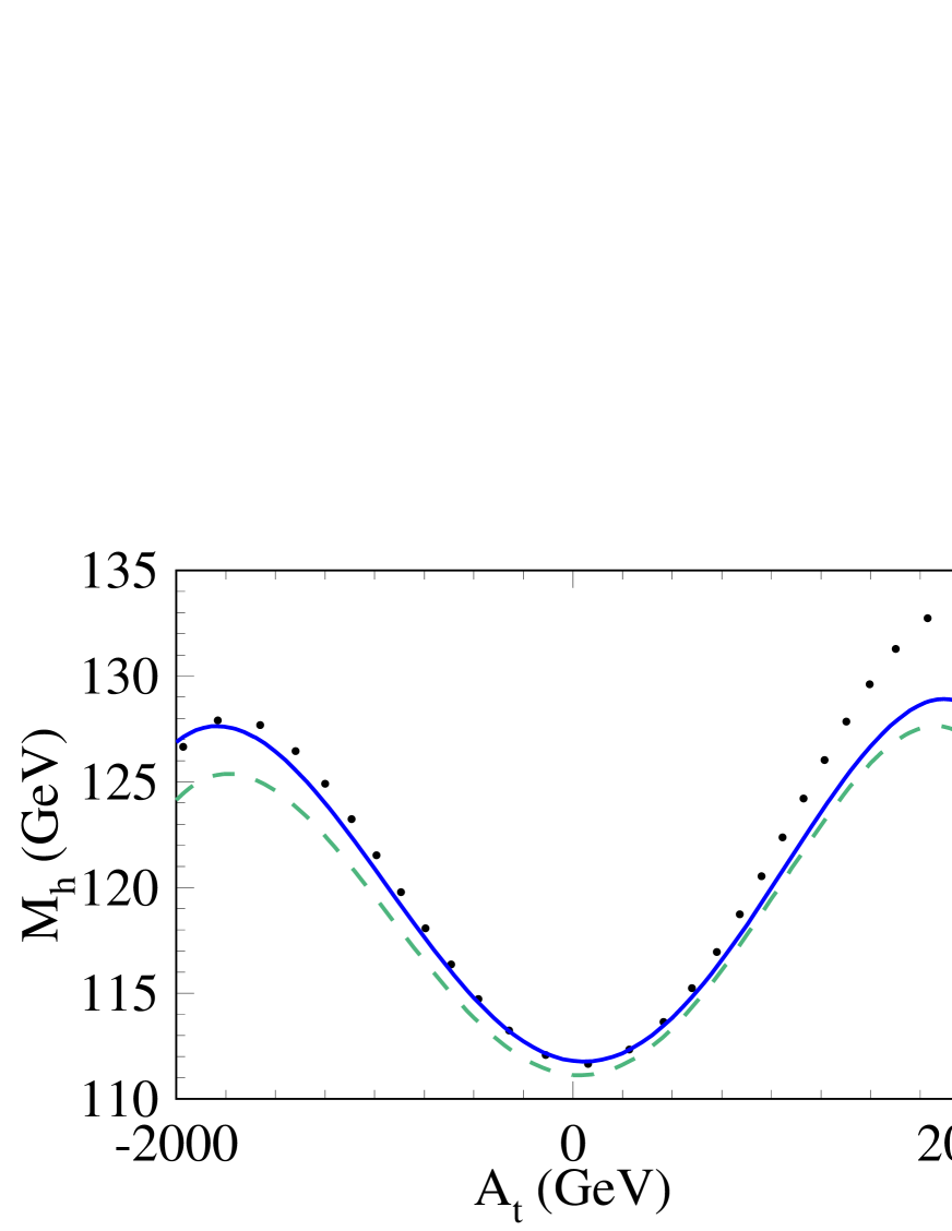
Refer to caption
Figure 11: Dependence of Mhsubscript𝑀M_{h} on Atsubscript𝐴𝑡A_{t}. The dotted, dashed and solid line corresponds to the one-, two- and three-loop prediction.

It is interesting to investigate the dependence of Mhsubscript𝑀M_{h} on the soft breaking parameter Atsubscript𝐴𝑡A_{t}. In Fig. 11 we show the result for Mhsubscript𝑀M_{h} where the following values for the parameters have been chosen

mt~1subscript𝑚subscript~𝑡1\displaystyle m_{\tilde{t}_{1}} =\displaystyle= 500GeV,500GeV\displaystyle 500~{}\mbox{GeV}\,,
mt~2subscript𝑚subscript~𝑡2\displaystyle m_{\tilde{t}_{2}} =\displaystyle= 1000GeV,1000GeV\displaystyle 1000~{}\mbox{GeV}\,,
mg~subscript𝑚~𝑔\displaystyle m_{\tilde{g}} =\displaystyle= 500GeV,500GeV\displaystyle 500~{}\mbox{GeV}\,,
mq~subscript𝑚~𝑞\displaystyle m_{\tilde{q}} =\displaystyle= 2000GeV,2000GeV\displaystyle 2000~{}\mbox{GeV}\,,
μSUSYsubscript𝜇SUSY\displaystyle\mu_{\rm SUSY} =\displaystyle= 800GeV,800GeV\displaystyle 800~{}\mbox{GeV}\,,
tanβ𝛽\displaystyle\tan\beta =\displaystyle= 10,10\displaystyle 10\,,
MAsubscript𝑀𝐴\displaystyle M_{A} =\displaystyle= 1500GeV.1500GeV\displaystyle 1500~{}\mbox{GeV}\,. (29)

Furthermore, we employ only the mt4superscriptsubscript𝑚𝑡4m_{t}^{4} corrections since it is not possible to transmit the parameters of Eq. (29) directly to FeynHiggs and evaluate the corresponding Higgs boson mass.

It is interesting to note that the three-loop corrections are quite sizeable, amounting up to about 3 GeV. In contrast to the two-loop terms they are positive and lead to a compensation. For At=2subscript𝐴𝑡2A_{t}=-2 TeV and At=0subscript𝐴𝑡0A_{t}=0 the three-loop prediction is even above the one-loop value for Mhsubscript𝑀M_{h}.

Refer to caption
Refer to caption
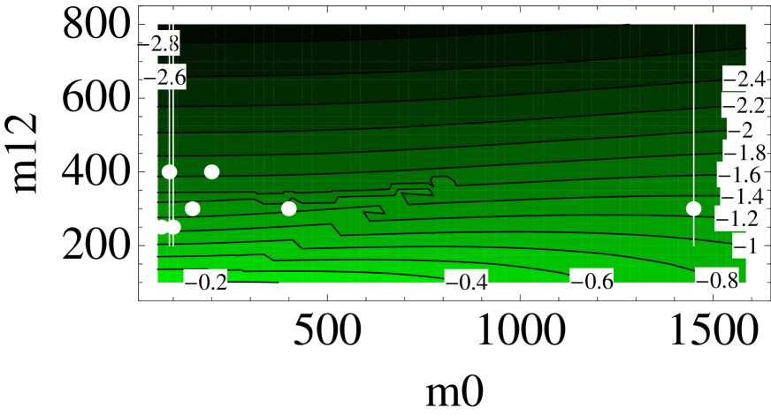
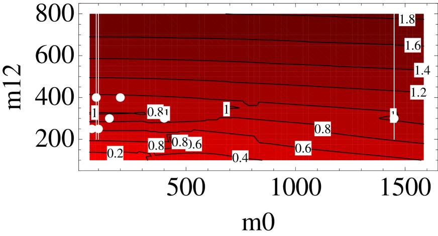
Figure 12: Genuine two- (upper panel) and three-loop (lower panel) corrections to Mhsubscript𝑀M_{h} in the m0subscript𝑚0m_{0}-m1/2subscript𝑚12m_{1/2} plane.
Refer to caption
Figure 13: Prediction of Mhsubscript𝑀M_{h} to three-loop accuracy using H3m. The same conventions as in Fig. 12 have been adopted.

In order to get an impression on the size of the three-loop corrections we show in Fig. 12 (lower panel) the difference between our best three-loop prediction and the full two-loop result as a function of m0subscript𝑚0m_{0} and m1/2subscript𝑚12m_{1/2}. We observe that the corrections are always positive and vary for our parameters between a few hundred MeV and about 2 GeV. They show only a mild dependence on m0subscript𝑚0m_{0}, but vary strongly with m1/2subscript𝑚12m_{1/2}. In particular the corrections become larger for increasing values of m1/2subscript𝑚12m_{1/2}. For comparison, we show in Fig. 12 (upper panel) the corresponding quantity at two-loop order, i.e., the difference between the two-loop and the one-loop result. In contrast to the three-loop contributions they are negative and amount to about twice the three-loop terms in a large region of the parameter space. However, there are also regions where the three-loop corrections are larger than the two-loop ones. Note, however, that in the whole m0subscript𝑚0m_{0}-m1/2subscript𝑚12m_{1/2} plane the one-loop corrections are more than ten times bigger. Furthermore, the occurrence of three-loop corrections, which are large compared to the two-loop ones, can also be seen from Fig. 10(d): whereas the two-loop corrections vary between 44-4 GeV and +44+4 GeV in the considered range of μrsubscript𝜇𝑟\mu_{r} the three-loop term is almost constant and amounts to about 1 GeV relative to the two-loop result.

In Fig. 13 we finally show the three-loop prediction of Mhsubscript𝑀M_{h} including the three-loop effects discussed in this paper. Again we restrict ourselves to the parameter space defined above. Values for other input parameters are easily obtained with the help of H3m. One can see that for increasing m1/2subscript𝑚12m_{1/2} also the Higgs boson mass gets larger and values well above 120 GeV can be reached. This is already observed at one-loop order and is due to the fact that for larger values of m1/2subscript𝑚12m_{1/2} the whole supersymmetric spectrum becomes heavier. For definiteness we show in Tab. 3 the three-loop prediction of Mhsubscript𝑀M_{h} for the SPS points. We show the best prediction (Mh(3)superscriptsubscript𝑀3M_{h}^{(3)}) and, for comparison, the result obtained by cutting parameters as for Fig. 9 (Mh(3),cutsuperscriptsubscript𝑀3cutM_{h}^{(3),\rm cut}). Furthermore, we indicate the optimal hierarchy as chosen by H3m. In all cases the uncertainty due to our approximation can be estimated to be below 100 MeV.

Mh(3)superscriptsubscript𝑀3M_{h}^{(3)} Mh(3),cutsuperscriptsubscript𝑀3cutM_{h}^{(3),\rm cut} optimal
(GeV) (GeV) hierarchy
SPS1a 112.46 112.45 h6b
SPS1a 113.92 113.92 h6b
SPS1b 116.49 116.44 h3
SPS2 116.67 116.61 h5
SPS3 115.59 115.52 h3
SPS4 114.82 114.81 h6
SPS5 112.02 111.92 h3
SPS7 113.04 113.04 h3
SPS8 115.03 115.02 h3
Table 3: Comparison of the best three-loop prediction to the one where some expansion parameters are cut (see text). The last column shows the chosen hierarchy.

As a last phenomenological application we consider the benchmark points identified in Ref. [53] in order to perform the MSSM Higgs boson search at hadron colliders. In Tab. 4 the one-, two- and three-loop predictions for Mhsubscript𝑀M_{h} are shown for the four scenarios “mhmaxsuperscriptsubscript𝑚maxm_{h}^{\rm max}”, “no-mixing”, “gluophobic” and “small αeffsubscript𝛼eff\alpha_{\rm eff}”. Whereas for “no-mixing” significant three-loop effects are observed more moderate, however, still important contributions are obtained for the remaining three scenarios. In Tab. 4 tanβ=10𝛽10\tan\beta=10 and MA=1500subscript𝑀𝐴1500M_{A}=1500 GeV has been chosen, however, a similar conclusion can be drawn for other values.

scenario 1 loop 2 loops 3 loops
mhmaxsuperscriptsubscript𝑚maxm_{h}^{\rm max} 141.11 133.96 134.38
no-mixing 121.33 119.72 121.07
gluophobic 118.52 117.47 117.29
small αeffsubscript𝛼eff\alpha_{\rm eff} 120.20 118.33 119.10
Table 4: Results for Mhsubscript𝑀M_{h} (in GeV) for the benchmark scenarios defined in Ref. [53] where tanβ=10𝛽10\tan\beta=10 and MA=1500subscript𝑀𝐴1500M_{A}=1500 GeV has been chosen.

Let us at the end of this Section estimate the theoretical uncertainty on the prediction of Mhsubscript𝑀M_{h} after including the three-loop corrections. We divide the uncertainty into two parts: (i)𝑖(i) the theoretical error due to missing higher order corrections and other as of yet uncalculated corrections, and (ii)𝑖𝑖(ii) the parametric uncertainty, mainly due to the top quark mass, αssubscript𝛼𝑠\alpha_{s} and the supersymmetric masses. At two-loop level, a thorough investigation of the theoretical uncertainties (i) has been performed in Ref. [9] (for earlier work, see Ref. [15]). It was found that missing two-loop corrections (most importantly electro-weak and finite-momentum effects) can be assumed to be well below 1 GeV, while the as of then unknown three-loop effects could amount to 2-3 GeV, as indicated by the variation of the two-loop results with the renormalization scale.

With the αtαs2subscript𝛼𝑡superscriptsubscript𝛼𝑠2\alpha_{t}\alpha_{s}^{2} corrections of our calculation, we should therefore be able to reduce the theory uncertainty. Instead of renormalization scale variations, however, we want to adopt a more conservative attitude and assume a geometric progression of the perturbative series. As can be confirmed at two-loop level, a conservative estimate of the uncertainty is 50% of the difference to the next lower order. Thus we assign 50% of the three-loop contribution to Mhsubscript𝑀M_{h} as a theoretical error. For the msugra scenarios this leads to an uncertainty of about 100200100200100-200 MeV for m1/2=100subscript𝑚12100m_{1/2}=100 GeV and to about 1 GeV for m1/2=1subscript𝑚121m_{1/2}=1 TeV. These estimates cover also corrections from renormalization group improvements which at two-loop order lead to shifts in Mhsubscript𝑀M_{h} of the order of a few GeV [Carena:2000dp].

Earlier in this section, we have identified two more contributions to the uncertainties of type (i): The corrections beyond the quartic top quark mass contribution, ΔremMh(3)superscriptΔremsuperscriptsubscript𝑀3\Delta^{\rm rem}M_{h}^{(3)}, has been estimated to about 100100100 MeV and the uncertainty due to our approximation procedure also amounts to at most 100100100 MeV. Both contributions are smaller than the one due to missing higher order corrections discussed above.

The parametric uncertainties can be easily estimated with the help of H3m. For definiteness we adopt in the following SPS2 and vary Mtsubscript𝑀𝑡M_{t} and αs(MZ)subscript𝛼𝑠subscript𝑀𝑍\alpha_{s}(M_{Z}) as follows

Mtsubscript𝑀𝑡\displaystyle M_{t} =\displaystyle= 173.1±1.3GeV,plus-or-minus173.11.3GeV\displaystyle 173.1\pm 1.3~{}\mbox{GeV}\,, (30)
αs(MZ)subscript𝛼𝑠subscript𝑀𝑍\displaystyle\alpha_{s}(M_{Z}) =\displaystyle= 0.1184±0.0020.plus-or-minus0.11840.0020\displaystyle 0.1184\pm 0.0020\,. (31)

In the case of the top quark mass we observe for m1/2=100subscript𝑚12100m_{1/2}=100 GeV a variation of Mhsubscript𝑀M_{h} by about 350 MeV which increases to δMh=1𝛿subscript𝑀1\delta M_{h}=1 GeV for m1/2=1subscript𝑚121m_{1/2}=1 TeV. The corresponding numbers for the uncertainty in αs(MZ)subscript𝛼𝑠subscript𝑀𝑍\alpha_{s}(M_{Z}) read 80 MeV and 600 MeV. A further uncertainty is connected to the (unknown) supersymmetric parameters which may also be of the order of a few hundred MeV. Assuming, e.g., an uncertainty of 10% for mt~1subscript𝑚subscript~𝑡1m_{\tilde{t}_{1}} in the range between 200 and 800 GeV and adopting the remaining parameters from Eq. (29) leads to an uncertainty of at most 500 MeV for Mhsubscript𝑀M_{h}. Note that the parametric uncertainty is of the same order of magnitude as the theoretical error due to missing higher order corrections as estimated in the previous paragraph.

6 Conclusions

In this paper we have discussed the lightest Higgs boson mass of the MSSM to three-loop accuracy. At this order an exact calculation is out of range and thus we heavily exploit the methods of asymptotic expansion in order to provide precise approximations. This procedure has been successfully tested at two-loop order against the full result. The result is expressed in terms of DR¯¯DR\overline{\mbox{DR}} parameters for the quark and squark masses for which we have found very good convergence of the perturbative expansion. We provide a user-friendly Mathematica program H3m which allows the computation of Mhsubscript𝑀M_{h} in a simple way. In particular, it is possible to apply various SUSY breaking scanarios, invoke a spectrum generator, and use the output in order to compute Mhsubscript𝑀M_{h}.

As already mentioned, with the help of the asymptotic expansion we have implemented analytical results valid for various hierarchies in the supersymmetric masses. H3m is set up in such a way that it is straightforward to include further hierarchies in case they are needed for future investigations.

We have performed several studies with the new three-loop corrections. In particular, we have considered their renormalization scheme and scale dependence, and their numerical effect in the various SPS scenarios. Furthermore, assuming msugra, we have considered the m0subscript𝑚0m_{0}-m1/2subscript𝑚12m_{1/2} parameter space and computed two and three-loop corrections. On the basis of these investigations we estimate the remaining theory uncertainty of Mhsubscript𝑀M_{h} to about 200 MeV for m1/2=100subscript𝑚12100m_{1/2}=100 GeV and to about 1 GeV for m1/2=1subscript𝑚121m_{1/2}=1 TeV.

Acknowledgements

We thank Steven Martin for providing us with C++ routines for the relation between the DR¯¯DR\overline{\mbox{DR}} and on-shell top quark mass, and Pietro Slavich for providing us with the analytic result for the two-loop SQCD corrections. We are grateful to Sven Heinemeyer for carefully reading the manuscript and many valuable comments, and to Thomas Hermann for useful comments on Appendix A. This work was supported by the DFG through SFB/TR 9 “Computational Particle Physics” and contract HA 2990/3-1, and by the Helmholtz Alliance “Physics at the Terascale”.

Appendix A: DR¯¯DR\overline{\rm DR} counterterms

In this appendix we provide details about the computation of the counterterms for the gluino, top quark and squark masses and the mixing angle in the top squark system.

To define our framework for the computation of the top squark masses and mixing angle counterterms, we start from the bare Lagrangian containing the kinetic energy and mass terms

t~(0)=12μ(t~L,t~R)(0)μ(t~Lt~R)(0)12(t~L,t~R)(0)(t~2)(0)(t~Lt~R)(0),superscriptsubscript~𝑡012subscript𝜇superscriptsuperscriptsubscript~𝑡𝐿superscriptsubscript~𝑡𝑅0superscript𝜇superscriptsubscript~𝑡𝐿subscript~𝑡𝑅012superscriptsuperscriptsubscript~𝑡𝐿superscriptsubscript~𝑡𝑅0superscriptsuperscriptsubscript~𝑡20superscriptsubscript~𝑡𝐿subscript~𝑡𝑅0\displaystyle{\cal L}_{\tilde{t}}^{(0)}=\frac{1}{2}\partial_{\mu}(\tilde{t}_{L}^{\ast},\tilde{t}_{R}^{\ast})^{(0)}\partial^{\mu}\left(\begin{array}[]{c}\tilde{t}_{L}\\ \tilde{t}_{R}\end{array}\right)^{\!\!(0)}-\frac{1}{2}(\tilde{t}_{L}^{\ast},\tilde{t}_{R}^{\ast})^{(0)}({\cal M}_{{\tilde{t}}}^{2})^{(0)}\left(\begin{array}[]{c}\tilde{t}_{L}\\ \tilde{t}_{R}\end{array}\right)^{\!\!(0)}\,, (36)

where the superscript (0)0(0) labels the bare quantities, t~Lsubscript~𝑡𝐿\tilde{t}_{L} and t~Rsubscript~𝑡𝑅\tilde{t}_{R} denote the interaction eigenstates and the top squark mass matrix was defined in Eq. (12).

The top squark mass eigenstates are related to the interaction eigenstates by

(t~1t~2)(0)=t~(0)(t~Lt~R)(0),superscriptsubscript~𝑡1subscript~𝑡20superscriptsubscript~𝑡0superscriptsubscript~𝑡𝐿subscript~𝑡𝑅0\displaystyle\left(\begin{array}[]{c}\tilde{t}_{1}\\ \tilde{t}_{2}\end{array}\right)^{\!\!(0)}={\cal R}_{{\tilde{t}}}^{(0)\,{\dagger}}\left(\begin{array}[]{c}\tilde{t}_{L}\\ \tilde{t}_{R}\end{array}\right)^{\!\!(0)}\,, (41)

where the matrix t~subscript~𝑡{\cal R}_{{\tilde{t}}} is defined in Eq. (18).

The wave function renormalization can be written in matrix form

(t~1t~2)(0)=𝒵t~1/2(t~1t~2),with𝒵t~1/2=(Z111/2Z121/2Z211/2Z221/2),formulae-sequencesuperscriptsubscript~𝑡1subscript~𝑡20superscriptsubscript𝒵~𝑡12subscript~𝑡1subscript~𝑡2withsuperscriptsubscript𝒵~𝑡12superscriptsubscript𝑍1112superscriptsubscript𝑍1212superscriptsubscript𝑍2112superscriptsubscript𝑍2212\displaystyle\left(\begin{array}[]{c}\tilde{t}_{1}\\ \tilde{t}_{2}\end{array}\right)^{\!\!(0)}={\cal Z}_{\tilde{t}}^{1/2}\left(\begin{array}[]{c}\tilde{t}_{1}\\ \tilde{t}_{2}\end{array}\right)\,,\quad\mbox{with}\quad{\cal Z}_{\tilde{t}}^{1/2}=\left(\begin{array}[]{cc}Z_{11}^{1/2}&Z_{12}^{1/2}\\ Z_{21}^{1/2}&Z_{22}^{1/2}\end{array}\right)\,, (48)

where we have 𝒵t~1/2=𝐈+𝒪(αs)superscriptsubscript𝒵~𝑡12𝐈𝒪subscript𝛼𝑠{\cal Z}_{\tilde{t}}^{1/2}=\mathbf{I}+{\cal O}(\alpha_{s}). Thus, Z111/2=1+𝒪(αs)superscriptsubscript𝑍11121𝒪subscript𝛼𝑠Z_{11}^{1/2}=1+{\cal O}(\alpha_{s}), Z221/2=1+𝒪(αs)superscriptsubscript𝑍22121𝒪subscript𝛼𝑠Z_{22}^{1/2}=1+{\cal O}(\alpha_{s}), Z121/2=𝒪(αs)superscriptsubscript𝑍1212𝒪subscript𝛼𝑠Z_{12}^{1/2}={\cal O}(\alpha_{s}) and Z211/2=𝒪(αs)superscriptsubscript𝑍2112𝒪subscript𝛼𝑠Z_{21}^{1/2}={\cal O}(\alpha_{s}).
Similarly, the renormalized mass matrix can be parametrized as follows

(mt~1200mt~22)(0)=(m112Zm11m122Zm12m212Zm21m222Zm22),superscriptsuperscriptsubscript𝑚subscript~𝑡1200superscriptsubscript𝑚subscript~𝑡220superscriptsubscript𝑚112subscript𝑍subscript𝑚11superscriptsubscript𝑚122subscript𝑍subscript𝑚12superscriptsubscript𝑚212subscript𝑍subscript𝑚21superscriptsubscript𝑚222subscript𝑍subscript𝑚22\displaystyle\left(\begin{array}[]{cc}m_{\tilde{t}_{1}}^{2}&0\\ 0&m_{\tilde{t}_{2}}^{2}\end{array}\right)^{\!\!(0)}=\left(\begin{array}[]{cc}m_{11}^{2}Z_{m_{11}}&m_{12}^{2}Z_{m_{12}}\\ m_{21}^{2}Z_{m_{21}}&m_{22}^{2}Z_{m_{22}}\end{array}\right)\equiv{\cal M}\,, (53)

where the mijsubscript𝑚𝑖𝑗m_{ij} stand for renormalized mass parameters.

In order to extract the renormalization constants it is convenient to consider the renormalized inverse top squark propagator which reads

iS1(p2)=p2(𝒵t~1/2)𝒵t~1/2(𝒵t~1/2)[Σ(p2)]𝒵t~1/2,𝑖superscript𝑆1superscript𝑝2superscript𝑝2superscriptsuperscriptsubscript𝒵~𝑡12superscriptsubscript𝒵~𝑡12superscriptsuperscriptsubscript𝒵~𝑡12delimited-[]Σsuperscript𝑝2superscriptsubscript𝒵~𝑡12\displaystyle iS^{-1}(p^{2})=p^{2}({\cal Z}_{\tilde{t}}^{1/2})^{\dagger}{\cal Z}_{\tilde{t}}^{1/2}-({\cal Z}_{\tilde{t}}^{1/2})^{\dagger}[{\cal M}-\Sigma(p^{2})]{\cal Z}_{\tilde{t}}^{1/2}\,, (54)

where Σ(p2)Σsuperscript𝑝2\Sigma(p^{2}) denotes the matrix of self energies constructed by the t~1subscript~𝑡1\tilde{t}_{1} and t~2subscript~𝑡2\tilde{t}_{2} fields.

To determine the renormalization constants introduced above one has to specify the renormalization conditions. In the DR¯¯DR\overline{\mbox{DR}} scheme the finite parts of the renormalization constants are set to zero and the coefficients of the ϵitalic-ϵ\epsilon poles are obtained from the requirements

iSij1(p2)|ppevaluated-at𝑖superscriptsubscript𝑆𝑖𝑗1superscript𝑝2pp\displaystyle iS_{ij}^{-1}(p^{2})\bigg{|}_{\rm pp} =\displaystyle= 0,0\displaystyle 0\,,
m122Zm12=m212Zm21superscriptsubscript𝑚122subscript𝑍subscript𝑚12superscriptsubscript𝑚212subscript𝑍subscript𝑚21\displaystyle m_{12}^{2}Z_{m_{12}}\,\,=\,\,m_{21}^{2}Z_{m_{21}} =\displaystyle= 0,0\displaystyle 0\,, (55)

where “pp” stands for the “pole part”. The conditions in the second line of Eq. (55) ensure that the renormalized fields t~1subscript~𝑡1\tilde{t}_{1} and t~2subscript~𝑡2\tilde{t}_{2} are the mass eigenstates of the renormalized mass matrix. Accordingly, we can identify Zm11subscript𝑍subscript𝑚11Z_{m_{11}} and Zm22subscript𝑍subscript𝑚22Z_{m_{22}} with the DR¯¯DR\overline{\mbox{DR}} renormalization constants Zmt~1subscript𝑍subscript𝑚subscript~𝑡1Z_{m_{\tilde{t}_{1}}} and Zmt~2subscript𝑍subscript𝑚subscript~𝑡2Z_{m_{\tilde{t}_{2}}} defined through

(mt~i2)(0)=mt~i2Zmt~i,i=1,2.formulae-sequencesuperscriptsuperscriptsubscript𝑚subscript~𝑡𝑖20superscriptsubscript𝑚subscript~𝑡𝑖2subscript𝑍subscript𝑚subscript~𝑡𝑖𝑖12\displaystyle(m_{\tilde{t}_{i}}^{2})^{(0)}=m_{\tilde{t}_{i}}^{2}Z_{m_{\tilde{t}_{i}}}\,,\quad i=1,2\,. (56)

In the DR¯¯DR\overline{\mbox{DR}} scheme the wave function renormalization constants are independent of the masses, so we can evaluate them solving Eqs. (55) for mt~1=mt~2=0subscript𝑚subscript~𝑡1subscript𝑚subscript~𝑡20m_{\tilde{t}_{1}}=m_{\tilde{t}_{2}}=0. In addition, we can exploit the symmetry of the matrix 𝒵t~1/2superscriptsubscript𝒵~𝑡12{\cal Z}_{\tilde{t}}^{1/2} and reparametrize it in terms of the common wave-function renormalization constant of the fields t~1subscript~𝑡1\tilde{t}_{1} and t~2subscript~𝑡2\tilde{t}_{2} and the counterterm of the mixing angle, as follows

𝒵t~1/2Z~21/2(cosδθtsinδθtsinδθtcosδθt).superscriptsubscript𝒵~𝑡12superscriptsubscript~𝑍212𝛿subscript𝜃𝑡𝛿subscript𝜃𝑡𝛿subscript𝜃𝑡𝛿subscript𝜃𝑡\displaystyle{\cal Z}_{\tilde{t}}^{1/2}\equiv\tilde{Z}_{2}^{1/2}\left(\begin{array}[]{cc}\cos\delta\theta_{t}&\sin\delta\theta_{t}\\ -\sin\delta\theta_{t}&\cos\delta\theta_{t}\end{array}\right)\,. (59)

We solve Eqs. (55) iteratively by inserting the perturbative expansion of all quantities,

Z𝑍\displaystyle Z =\displaystyle= 1+αsπδZ(1)+(αsπ)2δZ(2)+𝒪(αs3),1subscript𝛼𝑠𝜋𝛿superscript𝑍1superscriptsubscript𝛼𝑠𝜋2𝛿superscript𝑍2𝒪superscriptsubscript𝛼𝑠3\displaystyle 1+\frac{\alpha_{s}}{\pi}\delta Z^{(1)}+\left(\frac{\alpha_{s}}{\pi}\right)^{2}\delta Z^{(2)}+{\cal O}(\alpha_{s}^{3})\,,
δθt𝛿subscript𝜃𝑡\displaystyle\delta\theta_{t} =\displaystyle= αsπδθt(1)+(αsπ)2δθt(2)+𝒪(αs3),subscript𝛼𝑠𝜋𝛿superscriptsubscript𝜃𝑡1superscriptsubscript𝛼𝑠𝜋2𝛿superscriptsubscript𝜃𝑡2𝒪superscriptsubscript𝛼𝑠3\displaystyle\frac{\alpha_{s}}{\pi}\delta\theta_{t}^{(1)}+\left(\frac{\alpha_{s}}{\pi}\right)^{2}\delta\theta_{t}^{(2)}+{\cal O}(\alpha_{s}^{3})\,,
ΣijsubscriptΣ𝑖𝑗\displaystyle\Sigma_{ij} =\displaystyle= αsπΣij(1)+(αsπ)2Σij(2)+𝒪(αs3),i,j=1,2,formulae-sequencesubscript𝛼𝑠𝜋superscriptsubscriptΣ𝑖𝑗1superscriptsubscript𝛼𝑠𝜋2superscriptsubscriptΣ𝑖𝑗2𝒪superscriptsubscript𝛼𝑠3𝑖𝑗12\displaystyle\frac{\alpha_{s}}{\pi}\Sigma_{ij}^{(1)}+\left(\frac{\alpha_{s}}{\pi}\right)^{2}\Sigma_{ij}^{(2)}+{\cal O}(\alpha_{s}^{3})\,,\quad i,j=1,2\,, (60)

and take into account the reparametrization of Eq. (59). At one-loop order we get

[Σii(1)mt~i2(δZ2(1)+δZmt~i(1))+p2δZ2(1)]|ppevaluated-atdelimited-[]superscriptsubscriptΣ𝑖𝑖1superscriptsubscript𝑚subscript~𝑡𝑖2𝛿superscriptsubscript𝑍21𝛿superscriptsubscript𝑍subscript𝑚subscript~𝑡𝑖1superscript𝑝2𝛿superscriptsubscript𝑍21pp\displaystyle\left[\Sigma_{ii}^{(1)}-m_{\tilde{t}_{i}}^{2}(\delta Z_{2}^{(1)}+\delta Z_{m_{\tilde{t}_{i}}}^{(1)})+p^{2}\delta Z_{2}^{(1)}\right]\bigg{|}_{\rm pp} =\displaystyle= 0,i=1,2,formulae-sequence0𝑖12\displaystyle 0\,,\quad i=1,2\,,
[Σ12(1)δθt(1)(mt~12mt~22)]|ppevaluated-atdelimited-[]superscriptsubscriptΣ121𝛿superscriptsubscript𝜃𝑡1superscriptsubscript𝑚subscript~𝑡12superscriptsubscript𝑚subscript~𝑡22pp\displaystyle\left[\Sigma_{12}^{(1)}-\delta\theta_{t}^{(1)}(m_{\tilde{t}_{1}}^{2}-m_{\tilde{t}_{2}}^{2})\right]\bigg{|}_{\rm pp} =\displaystyle= 0.0\displaystyle 0\,. (61)

In a first step we solve the first equations with mt~1=mt~2=0subscript𝑚subscript~𝑡1subscript𝑚subscript~𝑡20m_{\tilde{t}_{1}}=m_{\tilde{t}_{2}}=0 to obtain

δZ2(1)𝛿superscriptsubscript𝑍21\displaystyle\delta Z_{2}^{(1)} =\displaystyle= 1p2Σii(1)(p)|pp,i=1ori=2.evaluated-at1superscript𝑝2superscriptsubscriptΣ𝑖𝑖1𝑝pp𝑖1or𝑖2\displaystyle-\frac{1}{p^{2}}\Sigma_{ii}^{(1)}(p)\bigg{|}_{\rm pp}\,,\quad i=1\,\,\mbox{or}\,\,i=2\,. (62)

Afterwards, we determine δZmt~i(1)𝛿superscriptsubscript𝑍subscript𝑚subscript~𝑡𝑖1\delta Z_{m_{\tilde{t}_{i}}}^{(1)} such that the equations are fulfilled also for finite mt~isubscript𝑚subscript~𝑡𝑖m_{\tilde{t}_{i}}. The renormalization conditions for S121superscriptsubscript𝑆121S_{12}^{-1} and S211superscriptsubscript𝑆211S_{21}^{-1} in Eq. (55) provide an expression for δθt(1)𝛿superscriptsubscript𝜃𝑡1\delta\theta_{t}^{(1)}:

δθt(1)𝛿superscriptsubscript𝜃𝑡1\displaystyle\delta\theta_{t}^{(1)} =\displaystyle= Σ12(1)mt~12mt~22|pp.evaluated-atsuperscriptsubscriptΣ121superscriptsubscript𝑚subscript~𝑡12superscriptsubscript𝑚subscript~𝑡22pp\displaystyle\frac{\Sigma_{12}^{(1)}}{m_{\tilde{t}_{1}}^{2}-m_{\tilde{t}_{2}}^{2}}\bigg{|}_{\rm pp}\,. (63)

Similarly, at two-loop order we have

[Σii(2)+Σii(1)δZ2(1)mt~i2(δZ2(2)+δZ2(1)δZmt~i(1)+δZmt~i(2))\displaystyle\Bigg{[}\Sigma_{ii}^{(2)}+\Sigma_{ii}^{(1)}\delta Z_{2}^{(1)}-m_{\tilde{t}_{i}}^{2}(\delta Z_{2}^{(2)}+\delta Z_{2}^{(1)}\delta Z_{m_{\tilde{t}_{i}}}^{(1)}+\delta Z_{m_{\tilde{t}_{i}}}^{(2)})
+(1)i+1δθt(1)[2Σ12(1)+δθt(1)(mt~12mt~22)]+p2δZ2(2)]|pp\displaystyle+(-1)^{i+1}\delta\theta_{t}^{(1)}[-2\Sigma_{12}^{(1)}+\delta\theta_{t}^{(1)}(m_{\tilde{t}_{1}}^{2}-m_{\tilde{t}_{2}}^{2})]+p^{2}\delta Z_{2}^{(2)}\Bigg{]}\bigg{|}_{\rm pp} =\displaystyle= 0(i=1,2),0𝑖12\displaystyle 0\quad(i=1,2)\,,
[Σ12(2)+Σ12(1)δZ2(1)+δθt(1)(Σ11(1)Σ22(1)mt~12δZmt~i(1)+mt~22δZmt~2(1))\displaystyle\Bigg{[}\Sigma_{12}^{(2)}+\Sigma_{12}^{(1)}\delta Z_{2}^{(1)}+\delta\theta_{t}^{(1)}(\Sigma_{11}^{(1)}-\Sigma_{22}^{(1)}-m_{\tilde{t}_{1}}^{2}\delta Z_{m_{\tilde{t}_{i}}}^{(1)}+m_{\tilde{t}_{2}}^{2}\delta Z_{m_{\tilde{t}_{2}}}^{(1)})
(mt~12mt~22)(δθt(2)+δθt(1)δZ2(1))]|pp\displaystyle-(m_{\tilde{t}_{1}}^{2}-m_{\tilde{t}_{2}}^{2})(\delta\theta_{t}^{(2)}+\delta\theta_{t}^{(1)}\delta Z_{2}^{(1)})\Bigg{]}\bigg{|}_{\rm pp} =\displaystyle= 0.0\displaystyle 0\,. (64)

In the following we list the results for the squark mass counterterms and the mixing angle, however, we refrain from providing explicit results for δZ2(1)𝛿superscriptsubscript𝑍21\delta Z_{2}^{(1)} and δZ2(2)𝛿superscriptsubscript𝑍22\delta Z_{2}^{(2)}, as we do not need them for the actual computation.

Our results for the renormalization constant of the top squark mass mt~1subscript𝑚subscript~𝑡1m_{\tilde{t}_{1}} read

mt~12δZmt~1(1)superscriptsubscript𝑚subscript~𝑡12𝛿superscriptsubscript𝑍subscript𝑚subscript~𝑡11\displaystyle m_{\tilde{t}_{1}}^{2}\delta Z_{{m}_{\tilde{t}_{1}}}^{(1)} =CF(mg~2mt2+mg~mtSt+mt~22mt~124St2)1ϵ,absentsubscript𝐶𝐹superscriptsubscript𝑚~𝑔2superscriptsubscript𝑚𝑡2subscript𝑚~𝑔subscript𝑚𝑡subscript𝑆𝑡superscriptsubscript𝑚subscript~𝑡22superscriptsubscript𝑚subscript~𝑡124superscriptsubscript𝑆𝑡21italic-ϵ\displaystyle=C_{F}\left(-m_{\tilde{g}}^{2}-m_{t}^{2}+m_{\tilde{g}}m_{t}S_{t}+\frac{m_{\tilde{t}_{2}}^{2}-m_{\tilde{t}_{1}}^{2}}{4}S_{t}^{2}\right)\frac{1}{\epsilon}\,,
mt~12δZmt~1(2)superscriptsubscript𝑚subscript~𝑡12𝛿superscriptsubscript𝑍subscript𝑚subscript~𝑡12\displaystyle m_{\tilde{t}_{1}}^{2}\delta Z_{{m}_{\tilde{t}_{1}}}^{(2)} ={CF2[Ct2mg~2mt2mt~12mt~22+(1+Ct2)St2(mt~12mt~22)+8mt216(1+Ct2)mg~mtSt2]\displaystyle=\bigg{\{}C_{F}^{2}\bigg{[}\frac{C_{t}^{2}m_{\tilde{g}}^{2}m_{t}^{2}}{m_{\tilde{t}_{1}}^{2}-m_{\tilde{t}_{2}}^{2}}+\frac{(1+C_{t}^{2})S_{t}^{2}(m_{\tilde{t}_{1}}^{2}-m_{\tilde{t}_{2}}^{2})+8m_{t}^{2}}{16}-\frac{(1+C_{t}^{2})m_{\tilde{g}}m_{t}S_{t}}{2}\bigg{]}
+CACF[9mg~28+3St2(mt~12mt~22)+4mt2323mg~mtSt4]subscript𝐶𝐴subscript𝐶𝐹delimited-[]9superscriptsubscript𝑚~𝑔283superscriptsubscript𝑆𝑡2superscriptsubscript𝑚subscript~𝑡12superscriptsubscript𝑚subscript~𝑡224superscriptsubscript𝑚𝑡2323subscript𝑚~𝑔subscript𝑚𝑡subscript𝑆𝑡4\displaystyle+C_{A}C_{F}\bigg{[}\frac{9m_{\tilde{g}}^{2}}{8}+3\frac{S_{t}^{2}(m_{\tilde{t}_{1}}^{2}-m_{\tilde{t}_{2}}^{2})+4m_{t}^{2}}{32}-\frac{3m_{\tilde{g}}m_{t}S_{t}}{4}\bigg{]}
+CFNfTF[3mg~24St2(mt~12mt~22)+4mt216+mg~mtSt2]}1ϵ2\displaystyle+C_{F}N_{f}T_{F}\bigg{[}\frac{-3m_{\tilde{g}}^{2}}{4}-\frac{S_{t}^{2}(m_{\tilde{t}_{1}}^{2}-m_{\tilde{t}_{2}}^{2})+4m_{t}^{2}}{16}+\frac{m_{\tilde{g}}m_{t}S_{t}}{2}\bigg{]}\bigg{\}}\frac{1}{\epsilon^{2}}
+{CF2[3mg~24+St2(mt~12mt~22)+4mt216mg~mtSt2]\displaystyle+\bigg{\{}C_{F}^{2}\bigg{[}\frac{3m_{\tilde{g}}^{2}}{4}+\frac{S_{t}^{2}(m_{\tilde{t}_{1}}^{2}-m_{\tilde{t}_{2}}^{2})+4m_{t}^{2}}{16}-\frac{m_{\tilde{g}}m_{t}S_{t}}{2}\bigg{]}
+CACF[11mg~283St2(mt~12mt~22)+4mt232+3mg~mtSt4]subscript𝐶𝐴subscript𝐶𝐹delimited-[]11superscriptsubscript𝑚~𝑔283superscriptsubscript𝑆𝑡2superscriptsubscript𝑚subscript~𝑡12superscriptsubscript𝑚subscript~𝑡224superscriptsubscript𝑚𝑡2323subscript𝑚~𝑔subscript𝑚𝑡subscript𝑆𝑡4\displaystyle+C_{A}C_{F}\bigg{[}\frac{-11m_{\tilde{g}}^{2}}{8}-3\frac{S_{t}^{2}(m_{\tilde{t}_{1}}^{2}-m_{\tilde{t}_{2}}^{2})+4m_{t}^{2}}{32}+\frac{3m_{\tilde{g}}m_{t}S_{t}}{4}\bigg{]}
+CFNqTF[3mg~24+St2(mt~12mt~22)+8mq~2+4mt216mg~mtSt2]subscript𝐶𝐹subscript𝑁𝑞subscript𝑇𝐹delimited-[]3superscriptsubscript𝑚~𝑔24superscriptsubscript𝑆𝑡2superscriptsubscript𝑚subscript~𝑡12superscriptsubscript𝑚subscript~𝑡228superscriptsubscript𝑚~𝑞24superscriptsubscript𝑚𝑡216subscript𝑚~𝑔subscript𝑚𝑡subscript𝑆𝑡2\displaystyle+C_{F}N_{q}T_{F}\bigg{[}\frac{3m_{\tilde{g}}^{2}}{4}+\frac{S_{t}^{2}(m_{\tilde{t}_{1}}^{2}-m_{\tilde{t}_{2}}^{2})+8m_{\tilde{q}}^{2}+4m_{t}^{2}}{16}-\frac{m_{\tilde{g}}m_{t}S_{t}}{2}\bigg{]}
+CFNtTF[3mg~24+St2(mt~12mt~22)+4mt~12+4mt~224mt216mg~mtSt2]}1ϵ\displaystyle+C_{F}N_{t}T_{F}\bigg{[}\frac{3m_{\tilde{g}}^{2}}{4}+\frac{S_{t}^{2}(m_{\tilde{t}_{1}}^{2}-m_{\tilde{t}_{2}}^{2})+4m_{\tilde{t}_{1}}^{2}+4m_{\tilde{t}_{2}}^{2}-4m_{t}^{2}}{16}-\frac{m_{\tilde{g}}m_{t}S_{t}}{2}\bigg{]}\bigg{\}}\frac{1}{\epsilon}
+Mε2(CACF38+CFNfTF14)1ϵ,superscriptsubscript𝑀𝜀2subscript𝐶𝐴subscript𝐶𝐹38subscript𝐶𝐹subscript𝑁𝑓subscript𝑇𝐹141italic-ϵ\displaystyle+M_{\varepsilon}^{2}\left(-C_{A}C_{F}\frac{3}{8}+C_{F}N_{f}T_{F}\frac{1}{4}\right)\frac{1}{\epsilon}\,, (65)

where we have introduced the abbreviations Nf=Nt+Nqsubscript𝑁𝑓subscript𝑁𝑡subscript𝑁𝑞N_{f}=N_{t}+N_{q}, St=sin2θtsubscript𝑆𝑡2subscript𝜃𝑡S_{t}=\sin 2\theta_{t} and Ct=cos2θtsubscript𝐶𝑡2subscript𝜃𝑡C_{t}=\cos 2\theta_{t}. Nqsubscript𝑁𝑞N_{q} denotes the number of light quark flavours and takes in our case the value Nq=5subscript𝑁𝑞5N_{q}=5. Nt=1subscript𝑁𝑡1N_{t}=1 has been introduced for convenience. Furthermore Mεsubscript𝑀𝜀M_{\varepsilon} denotes the on-shell renormalized ε𝜀\varepsilon-scalar mass. The corresponding results for mt~2subscript𝑚subscript~𝑡2m_{\tilde{t}_{2}} can be derived from Eq. (65) by interchanging mt~1subscript𝑚subscript~𝑡1m_{\tilde{t}_{1}} and mt~2subscript𝑚subscript~𝑡2m_{\tilde{t}_{2}} and changing the sign of θtsubscript𝜃𝑡\theta_{t}.

We have employed two different approaches for the renormalization of the ε𝜀\varepsilon-scalar mass. In one approach we renormalize it on-shell and choose Mε0subscript𝑀𝜀0M_{\varepsilon}\neq 0. In order to decouple the unphysical parameter Mεsubscript𝑀𝜀M_{\varepsilon} from the physical observables, i.e. Mhsubscript𝑀M_{h} in our case, we modify the top squark masses by a finite counterterm. This renormalization scheme is equivalent to the DR¯¯DR\overline{\mbox{DR}} scheme [54, 55]. However, in the original version of the DR¯¯DR\overline{\mbox{DR}} scheme the ε𝜀\varepsilon-scalar mass is renormalized minimally, whereas we choose the on-shell scheme. Thus, the finite counterterms we found differ starting from two-loops from the ones given in Ref. [55] by

δmt~i2𝛿superscriptsubscript𝑚subscript~𝑡𝑖2\displaystyle\delta m_{\tilde{t}_{i}}^{2} =\displaystyle= Mε2(αsπ)2[CF24+CACF34Lμε+Lμg~8\displaystyle M_{\varepsilon}^{2}\left(\frac{\alpha_{s}}{\pi}\right)^{2}\bigg{[}-\frac{C_{F}^{2}}{4}+C_{A}C_{F}\frac{-3-4L_{{\mu}\varepsilon}+L_{\mu\tilde{g}}}{8} (66)
+CFNqTF1+Lμε4+CFNtTF1+Lμt4],i=1,2,\displaystyle\mbox{}+C_{F}N_{q}T_{F}\frac{1+L_{{\mu}\varepsilon}}{4}+C_{F}N_{t}T_{F}\frac{-1+L_{{\mu}t}}{4}\bigg{]}\,,\quad i=1,2\,,

with Lμx=ln(μ2/mx2)subscript𝐿𝜇𝑥superscript𝜇2superscriptsubscript𝑚𝑥2L_{\mu x}=\ln(\mu^{2}/m_{x}^{2}) and Lμε=ln(μ2/Mε2)subscript𝐿𝜇𝜀superscript𝜇2superscriptsubscript𝑀𝜀2L_{{\mu}\varepsilon}=\ln(\mu^{2}/M_{\varepsilon}^{2}). In the second approach we set the on-shell ε𝜀\varepsilon-scalar mass to zero. Of course, no finite counterterm is needed in this case. The results for Mhsubscript𝑀M_{h} obtained employing the two methods are identical, however, the second approach is computationally less involved. Thus for the practical calculation we set the on-shell ε𝜀\varepsilon-scalar mass to zero.
Let us mention that strictly speaking our renormalization coincides neither DR¯¯DR\overline{\mbox{DR}} nor DR¯¯DR\overline{\mbox{DR}} due to the different treatment of the ε𝜀\varepsilon-scalar mass. Nevertheless we use the nomenclature “DR¯¯DR\overline{\mbox{DR}} scheme”.

Finally, for the mixing angle we have

((\displaystyle( mt~12mt~22)δθt(1)=CFCt(mg~mtSt(mt~12mt~22)4)1ϵ,\displaystyle m_{\tilde{t}_{1}}^{2}-m_{\tilde{t}_{2}}^{2})\delta\theta_{t}^{(1)}=C_{F}C_{t}\left(m_{\tilde{g}}m_{t}-\frac{S_{t}(m_{\tilde{t}_{1}}^{2}-m_{\tilde{t}_{2}}^{2})}{4}\right)\frac{1}{\epsilon}\,,
((\displaystyle( mt~12mt~22)δθt(2)={CF2Ct[(St2Ct2)(mg~mt2St(mt~12mt~22)16)2Stmg~2mt2mt~12mt~22]\displaystyle m_{\tilde{t}_{1}}^{2}-m_{\tilde{t}_{2}}^{2})\delta\theta_{t}^{(2)}=\bigg{\{}C_{F}^{2}C_{t}\bigg{[}(S_{t}^{2}-C_{t}^{2})\left(\frac{m_{\tilde{g}}m_{t}}{2}-\frac{S_{t}(m_{\tilde{t}_{1}}^{2}-m_{\tilde{t}_{2}}^{2})}{16}\right)-\frac{2S_{t}m_{\tilde{g}}^{2}m_{t}^{2}}{m_{\tilde{t}_{1}}^{2}-m_{\tilde{t}_{2}}^{2}}\bigg{]}
+CFCACt[3mg~mt4+3St(mt~12mt~22)32]+CFNfTFCt[mg~mt2St(mt~12mt~22)16]}1ϵ2\displaystyle+C_{F}C_{A}C_{t}\bigg{[}\frac{-3m_{\tilde{g}}m_{t}}{4}+\frac{3S_{t}(m_{\tilde{t}_{1}}^{2}-m_{\tilde{t}_{2}}^{2})}{32}\bigg{]}+C_{F}N_{f}T_{F}C_{t}\bigg{[}\frac{m_{\tilde{g}}m_{t}}{2}-\frac{S_{t}(m_{\tilde{t}_{1}}^{2}-m_{\tilde{t}_{2}}^{2})}{16}\bigg{]}\bigg{\}}\frac{1}{\epsilon^{2}}
+{CF2Ct[mg~mt2+St(mt~12mt~22)16]+CFCACt[3mg~mt43St(mt~12mt~22)32]\displaystyle+\bigg{\{}C_{F}^{2}C_{t}\bigg{[}-\frac{m_{\tilde{g}}m_{t}}{2}+\frac{S_{t}(m_{\tilde{t}_{1}}^{2}-m_{\tilde{t}_{2}}^{2})}{16}\bigg{]}+C_{F}C_{A}C_{t}\bigg{[}\frac{3m_{\tilde{g}}m_{t}}{4}-\frac{3S_{t}(m_{\tilde{t}_{1}}^{2}-m_{\tilde{t}_{2}}^{2})}{32}\bigg{]}
+CFNfTFCt[mg~mt2+St(mt~12mt~22)16]}1ϵ.\displaystyle+C_{F}N_{f}T_{F}C_{t}\bigg{[}-\frac{m_{\tilde{g}}m_{t}}{2}+\frac{S_{t}(m_{\tilde{t}_{1}}^{2}-m_{\tilde{t}_{2}}^{2})}{16}\bigg{]}\bigg{\}}\frac{1}{\epsilon}\,. (67)

The two-loop counterterms given in Eqs. (65) and (67) can also be derived from the more general results available in the literature  [56, 57, 58].

The on-shell renormalization constant of the ε𝜀\varepsilon-scalar mass to one-loop order is given by

(Mε2)(0)=Mε2ZMε2,ZMε2=1+αsπδZMε2(1)+𝒪(αs2),formulae-sequencesuperscriptsuperscriptsubscript𝑀𝜀20superscriptsubscript𝑀𝜀2subscript𝑍superscriptsubscript𝑀𝜀2subscript𝑍superscriptsubscript𝑀𝜀21subscript𝛼𝑠𝜋𝛿subscriptsuperscript𝑍1superscriptsubscript𝑀𝜀2𝒪superscriptsubscript𝛼𝑠2\displaystyle(M_{\varepsilon}^{2})^{(0)}=M_{\varepsilon}^{2}Z_{M_{\varepsilon}^{2}}\,,\quad Z_{M_{\varepsilon}^{2}}=1+\frac{\alpha_{s}}{\pi}\delta Z^{(1)}_{M_{\varepsilon}^{2}}+{\cal O}(\alpha_{s}^{2})\,, (68)

where

Mε2δZMε2(1)superscriptsubscript𝑀𝜀2𝛿subscriptsuperscript𝑍1superscriptsubscript𝑀𝜀2\displaystyle-M_{\varepsilon}^{2}\delta Z^{(1)}_{M_{\varepsilon}^{2}} =\displaystyle= [CA4(3Mε2+2mg~2)NqTF2(Mε2+2mq~2)NtTF2(Mε2+mt~12+mt~222mt2)]1ϵdelimited-[]subscript𝐶𝐴43superscriptsubscript𝑀𝜀22superscriptsubscript𝑚~𝑔2subscript𝑁𝑞subscript𝑇𝐹2superscriptsubscript𝑀𝜀22superscriptsubscript𝑚~𝑞2subscript𝑁𝑡subscript𝑇𝐹2superscriptsubscript𝑀𝜀2superscriptsubscript𝑚subscript~𝑡12superscriptsubscript𝑚subscript~𝑡222superscriptsubscript𝑚𝑡21italic-ϵ\displaystyle\bigg{[}\frac{C_{A}}{4}(3M_{\varepsilon}^{2}+2m_{\tilde{g}}^{2})-\frac{N_{q}T_{F}}{2}(M_{\varepsilon}^{2}+2m_{\tilde{q}}^{2})-\frac{N_{t}T_{F}}{2}(M_{\varepsilon}^{2}+m_{\tilde{t}_{1}}^{2}+m_{\tilde{t}_{2}}^{2}-2m_{t}^{2})\bigg{]}\frac{1}{\epsilon} (69)
+\displaystyle+ CA4[(6+4LμεLμg~)Mε2+2(1+Lμg~)mg~2]subscript𝐶𝐴4delimited-[]64subscript𝐿𝜇𝜀subscript𝐿𝜇~𝑔superscriptsubscript𝑀𝜀221subscript𝐿𝜇~𝑔superscriptsubscript𝑚~𝑔2\displaystyle\frac{C_{A}}{4}[(6+4L_{{\mu}\varepsilon}-L_{\mu\tilde{g}})M_{\varepsilon}^{2}+2(1+L_{\mu\tilde{g}})m_{\tilde{g}}^{2}]
\displaystyle- NqTF2[(2+Lμε)Mε2+2(1+Lμq~)mq~2]subscript𝑁𝑞subscript𝑇𝐹2delimited-[]2subscript𝐿𝜇𝜀superscriptsubscript𝑀𝜀221subscript𝐿𝜇~𝑞superscriptsubscript𝑚~𝑞2\displaystyle\frac{N_{q}T_{F}}{2}[(2+L_{{\mu}\varepsilon})M_{\varepsilon}^{2}+2(1+L_{\mu\tilde{q}})m_{\tilde{q}}^{2}]
\displaystyle- NtTF2[LμtMε2+(1+Lμt~1)mt~12+(1+Lμt~2)mt~222(1+Lμt)mt2].subscript𝑁𝑡subscript𝑇𝐹2delimited-[]subscript𝐿𝜇𝑡superscriptsubscript𝑀𝜀21subscript𝐿𝜇subscript~𝑡1superscriptsubscript𝑚subscript~𝑡121subscript𝐿𝜇subscript~𝑡2superscriptsubscript𝑚subscript~𝑡2221subscript𝐿𝜇𝑡superscriptsubscript𝑚𝑡2\displaystyle\frac{N_{t}T_{F}}{2}[L_{{\mu}t}M_{\varepsilon}^{2}+(1+L_{\mu\tilde{t}_{1}})m_{\tilde{t}_{1}}^{2}+(1+L_{\mu\tilde{t}_{2}})m_{\tilde{t}_{2}}^{2}-2(1+L_{{\mu}t})m_{t}^{2}]\,.

The two-loop renormalization constant for the top quark mass in the DR¯¯DR\overline{\mbox{DR}} scheme is known for long time [59, 60]. For the convenience of the reader we quote the results which are given by

mt(0)superscriptsubscript𝑚𝑡0\displaystyle m_{t}^{(0)} =\displaystyle= mtZmt,withZmt=1+αsπδZmt(1)+(αsπ)2δZmt(2)+𝒪(αs3),subscript𝑚𝑡subscript𝑍subscript𝑚𝑡withsubscript𝑍subscript𝑚𝑡1subscript𝛼𝑠𝜋𝛿superscriptsubscript𝑍subscript𝑚𝑡1superscriptsubscript𝛼𝑠𝜋2𝛿superscriptsubscript𝑍subscript𝑚𝑡2𝒪superscriptsubscript𝛼𝑠3\displaystyle m_{t}Z_{m_{t}}\,,\quad\mbox{with}\quad Z_{m_{t}}=1+\frac{\alpha_{s}}{\pi}\delta Z_{m_{t}}^{(1)}+\left(\frac{\alpha_{s}}{\pi}\right)^{2}\delta Z_{m_{t}}^{(2)}+{\cal O}(\alpha_{s}^{3})\,, (70)

and

δZmt(1)𝛿superscriptsubscript𝑍subscript𝑚𝑡1\displaystyle\delta Z_{m_{t}}^{(1)} =\displaystyle= CF12ϵ,subscript𝐶𝐹12italic-ϵ\displaystyle-C_{F}\frac{1}{2\epsilon}\,,
δZmt(2)𝛿superscriptsubscript𝑍subscript𝑚𝑡2\displaystyle\delta Z_{m_{t}}^{(2)} =\displaystyle= (18CF2+316CACF18CFNfTF)1ϵ218superscriptsubscript𝐶𝐹2316subscript𝐶𝐴subscript𝐶𝐹18subscript𝐶𝐹subscript𝑁𝑓subscript𝑇𝐹1superscriptitalic-ϵ2\displaystyle\left(\frac{1}{8}C_{F}^{2}+\frac{3}{16}C_{A}C_{F}-\frac{1}{8}C_{F}N_{f}T_{F}\right)\frac{1}{\epsilon^{2}} (71)
+\displaystyle+ (18CF2316CACF+18CFNfTF)1ϵ.18superscriptsubscript𝐶𝐹2316subscript𝐶𝐴subscript𝐶𝐹18subscript𝐶𝐹subscript𝑁𝑓subscript𝑇𝐹1italic-ϵ\displaystyle\left(\frac{1}{8}C_{F}^{2}-\frac{3}{16}C_{A}C_{F}+\frac{1}{8}C_{F}N_{f}T_{F}\right)\frac{1}{\epsilon}\,.

The same is true for the one-loop gluino mass counterterm [59, 60] defined through

mg~(0)=mg~Zmg~,withZmg~=1+αsπδZmg~(1)+𝒪(αs2),formulae-sequencesuperscriptsubscript𝑚~𝑔0subscript𝑚~𝑔subscript𝑍subscript𝑚~𝑔withsubscript𝑍subscript𝑚~𝑔1subscript𝛼𝑠𝜋𝛿superscriptsubscript𝑍subscript𝑚~𝑔1𝒪superscriptsubscript𝛼𝑠2\displaystyle m_{\tilde{g}}^{(0)}=m_{\tilde{g}}Z_{m_{\tilde{g}}}\,,\quad\mbox{with}\quad Z_{m_{\tilde{g}}}=1+\frac{\alpha_{s}}{\pi}\delta Z_{m_{\tilde{g}}}^{(1)}+{\cal O}(\alpha_{s}^{2})\,, (72)

with

δZmg~(1)𝛿superscriptsubscript𝑍subscript𝑚~𝑔1\displaystyle\delta Z_{m_{\tilde{g}}}^{(1)} =\displaystyle= (34CA+12NfTF)1ϵ.34subscript𝐶𝐴12subscript𝑁𝑓subscript𝑇𝐹1italic-ϵ\displaystyle\left(-\frac{3}{4}C_{A}+\frac{1}{2}N_{f}T_{F}\right)\frac{1}{\epsilon}\,. (73)

Appendix B: Modification of the DR¯¯DR\overline{\mbox{DR}} scheme: MDR¯¯MDR\overline{\mbox{MDR}}

As discussed in Section 3, the renormalization constants of the top squarks have mass dimension two. Thus, for some hierarchies considered in this paper parametrically (and numerically) large corrections might appear which are absent in the on-shell scheme. In order to cure this problem we introduce additional finite corrections in the corresponding renormalization constants which ensure that the renormalized result for the Higgs boson mass is free of these potentially dangerous contributions.

In the following we provide analytic expressions for the finite shifts introduced in the top squark mass counterterms as compared to the DR¯¯DR\overline{\mbox{DR}} scheme. According to the discussion in Section 3, one can distinguish three cases for the mass hierarchies.

Case (i): mq~mt~imuch-greater-thansubscript𝑚~𝑞subscript𝑚subscript~𝑡𝑖\quad m_{\tilde{q}}\gg m_{\tilde{t}_{i}}, (i=1,2)𝑖12(i=1,2)

(mt~iMDR¯mt~i)2superscriptsuperscriptsubscript𝑚subscript~𝑡𝑖¯MDRsubscript𝑚subscript~𝑡𝑖2\displaystyle\left(\frac{m_{\tilde{t}_{i}}^{\overline{\rm MDR}}}{m_{\tilde{t}_{i}}}\right)^{2} =\displaystyle= 1(αsπ)2CFNqTFmq~2mt~i2(12+Lμq~+ζ(2)).1superscriptsubscript𝛼𝑠𝜋2subscript𝐶𝐹subscript𝑁𝑞subscript𝑇𝐹superscriptsubscript𝑚~𝑞2superscriptsubscript𝑚subscript~𝑡𝑖212subscript𝐿𝜇~𝑞𝜁2\displaystyle 1-\left(\frac{\alpha_{s}}{\pi}\right)^{2}C_{F}N_{q}T_{F}\frac{m_{\tilde{q}}^{2}}{m_{\tilde{t}_{i}}^{2}}\left(-\frac{1}{2}+L_{\mu\tilde{q}}+\zeta(2)\right)\,. (74)

The label Nq=5subscript𝑁𝑞5N_{q}=5 has been introduced for convenience and for the logarithms the abbreviation Lμq~=ln(μ2/mq~2)subscript𝐿𝜇~𝑞superscript𝜇2superscriptsubscript𝑚~𝑞2L_{\mu\tilde{q}}=\ln(\mu^{2}/m_{\tilde{q}}^{2}) has been introduced.

Case (ii): mt~2mt~1much-greater-thansubscript𝑚subscript~𝑡2subscript𝑚subscript~𝑡1\quad m_{\tilde{t}_{2}}\gg m_{\tilde{t}_{1}}

(mt~1MDR¯mt~1)2superscriptsuperscriptsubscript𝑚subscript~𝑡1¯MDRsubscript𝑚subscript~𝑡12\displaystyle\left(\frac{m_{\tilde{t}_{1}}^{\overline{\rm MDR}}}{m_{\tilde{t}_{1}}}\right)^{2} =\displaystyle= 1(αsπ)2CFTFmt~22mt~12(14+12Lμt~2+12ζ(2)).1superscriptsubscript𝛼𝑠𝜋2subscript𝐶𝐹subscript𝑇𝐹superscriptsubscript𝑚subscript~𝑡22superscriptsubscript𝑚subscript~𝑡121412subscript𝐿𝜇subscript~𝑡212𝜁2\displaystyle 1-\left(\frac{\alpha_{s}}{\pi}\right)^{2}C_{F}T_{F}\frac{m_{\tilde{t}_{2}}^{2}}{m_{\tilde{t}_{1}}^{2}}\left(-\frac{1}{4}+\frac{1}{2}L_{\mu\tilde{t}_{2}}+\frac{1}{2}\zeta(2)\right)\,. (75)

In this equation we have Lμt~2=ln(μ2/mt~22)subscript𝐿𝜇subscript~𝑡2superscript𝜇2superscriptsubscript𝑚subscript~𝑡22L_{\mu\tilde{t}_{2}}=\ln(\mu^{2}/m_{\tilde{t}_{2}}^{2}).

Case (iii): mg~mt~imuch-greater-thansubscript𝑚~𝑔subscript𝑚subscript~𝑡𝑖\quad m_{\tilde{g}}\gg m_{\tilde{t}_{i}}, (i=1,2)𝑖12(i=1,2) and mq~mg~much-greater-thansubscript𝑚~𝑞subscript𝑚~𝑔m_{\tilde{q}}\gg m_{\tilde{g}}

(mt~iMDR¯mt~i)2superscriptsuperscriptsubscript𝑚subscript~𝑡𝑖¯MDRsubscript𝑚subscript~𝑡𝑖2\displaystyle\left(\frac{m_{\tilde{t}_{i}}^{\overline{\rm MDR}}}{m_{\tilde{t}_{i}}}\right)^{2} =\displaystyle= 1+αsπCF[1+Lμg~]mg~2mt~i2+(αsπ)2{CF2[11432Lμg~+ζ(2)]mg~2mt~i2\displaystyle 1+\frac{\alpha_{s}}{\pi}C_{F}\left[1+L_{\mu\tilde{g}}\right]\frac{m_{\tilde{g}}^{2}}{m_{\tilde{t}_{i}}^{2}}+\left(\frac{\alpha_{s}}{\pi}\right)^{2}\bigg{\{}C_{F}^{2}\left[-\frac{11}{4}-\frac{3}{2}L_{\mu\tilde{g}}+\zeta(2)\right]\frac{m_{\tilde{g}}^{2}}{m_{\tilde{t}_{i}}^{2}} (76)
+\displaystyle+ CACF[218+72Lμg~+98Lμg~214ζ(2)]mg~2mt~i2subscript𝐶𝐴subscript𝐶𝐹delimited-[]21872subscript𝐿𝜇~𝑔98superscriptsubscript𝐿𝜇~𝑔214𝜁2superscriptsubscript𝑚~𝑔2superscriptsubscript𝑚subscript~𝑡𝑖2\displaystyle C_{A}C_{F}\left[\frac{21}{8}+\frac{7}{2}L_{\mu\tilde{g}}+\frac{9}{8}L_{\mu\tilde{g}}^{2}-\frac{1}{4}\zeta(2)\right]\frac{m_{\tilde{g}}^{2}}{m_{\tilde{t}_{i}}^{2}}
+\displaystyle+ CFNtTF[(2+2Lμg~+34Lμg~2)mg~2mt~i2+(12ζ(2))mg~(mg~mt~2)mt~i2]subscript𝐶𝐹subscript𝑁𝑡subscript𝑇𝐹delimited-[]22subscript𝐿𝜇~𝑔34superscriptsubscript𝐿𝜇~𝑔2superscriptsubscript𝑚~𝑔2superscriptsubscript𝑚subscript~𝑡𝑖212𝜁2subscript𝑚~𝑔subscript𝑚~𝑔subscript𝑚subscript~𝑡2superscriptsubscript𝑚subscript~𝑡𝑖2\displaystyle C_{F}N_{t}T_{F}\left[-\left(2+2L_{\mu\tilde{g}}+\frac{3}{4}L_{\mu\tilde{g}}^{2}\right)\frac{m_{\tilde{g}}^{2}}{m_{\tilde{t}_{i}}^{2}}+\left(1-2\zeta(2)\right)\frac{m_{\tilde{g}}(m_{\tilde{g}}-m_{\tilde{t}_{2}})}{m_{\tilde{t}_{i}}^{2}}\right]
+\displaystyle+ CFNqTF[(5834Lμg~54Lμq~32Lμg~Lμq~+34Lμq~2+32ζ(2))mg~2mt~i2\displaystyle C_{F}N_{q}T_{F}\bigg{[}\left(-\frac{5}{8}-\frac{3}{4}L_{\mu\tilde{g}}-\frac{5}{4}L_{\mu\tilde{q}}-\frac{3}{2}L_{\mu\tilde{g}}L_{\mu\tilde{q}}+\frac{3}{4}L_{\mu\tilde{q}}^{2}+\frac{3}{2}\zeta(2)\right)\frac{m_{\tilde{g}}^{2}}{m_{\tilde{t}_{i}}^{2}}
+\displaystyle+ (433656Lq~g~)mg~4mq~2mt~i2+(67288724Lq~g~)mg~6mq~4mt~i2]}.\displaystyle\left(-\frac{43}{36}-\frac{5}{6}L_{\tilde{q}\tilde{g}}\right)\frac{m_{\tilde{g}}^{4}}{m_{\tilde{q}}^{2}m_{\tilde{t}_{i}}^{2}}+\left(-\frac{67}{288}-\frac{7}{24}L_{\tilde{q}\tilde{g}}\right)\frac{m_{\tilde{g}}^{6}}{m_{\tilde{q}}^{4}m_{\tilde{t}_{i}}^{2}}\bigg{]}\bigg{\}}\,.

Here Nt=1subscript𝑁𝑡1N_{t}=1, Lμg~=ln(μ2/mg~2)subscript𝐿𝜇~𝑔superscript𝜇2superscriptsubscript𝑚~𝑔2L_{\mu\tilde{g}}=\ln(\mu^{2}/m_{\tilde{g}}^{2}) and Lq~g~=ln(mq~2/mg~2)subscript𝐿~𝑞~𝑔superscriptsubscript𝑚~𝑞2superscriptsubscript𝑚~𝑔2L_{\tilde{q}\tilde{g}}=\ln(m_{\tilde{q}}^{2}/m_{\tilde{g}}^{2}).

Case (iv): mg~mt~imuch-greater-thansubscript𝑚~𝑔subscript𝑚subscript~𝑡𝑖\quad m_{\tilde{g}}\gg m_{\tilde{t}_{i}}, (i=1,2)𝑖12(i=1,2) and mq~mg~subscript𝑚~𝑞subscript𝑚~𝑔m_{\tilde{q}}\approx m_{\tilde{g}}

(mt~iMDR¯mt~i)2superscriptsuperscriptsubscript𝑚subscript~𝑡𝑖¯MDRsubscript𝑚subscript~𝑡𝑖2\displaystyle\left(\frac{m_{\tilde{t}_{i}}^{\overline{\rm MDR}}}{m_{\tilde{t}_{i}}}\right)^{2} =\displaystyle= 1+αsπCF[1+Lμg~]mg~2mt~i2+(αsπ)2{CF2[11432Lμg~+ζ(2)]mg~2mt~i2\displaystyle 1+\frac{\alpha_{s}}{\pi}C_{F}\left[1+L_{\mu\tilde{g}}\right]\frac{m_{\tilde{g}}^{2}}{m_{\tilde{t}_{i}}^{2}}+\left(\frac{\alpha_{s}}{\pi}\right)^{2}\bigg{\{}C_{F}^{2}\left[-\frac{11}{4}-\frac{3}{2}L_{\mu\tilde{g}}+\zeta(2)\right]\frac{m_{\tilde{g}}^{2}}{m_{\tilde{t}_{i}}^{2}} (77)
+\displaystyle+ CACF[218+72Lμg~+98Lμg~214ζ(2)]mg~2mt~i2subscript𝐶𝐴subscript𝐶𝐹delimited-[]21872subscript𝐿𝜇~𝑔98superscriptsubscript𝐿𝜇~𝑔214𝜁2superscriptsubscript𝑚~𝑔2superscriptsubscript𝑚subscript~𝑡𝑖2\displaystyle C_{A}C_{F}\left[\frac{21}{8}+\frac{7}{2}L_{\mu\tilde{g}}+\frac{9}{8}L_{\mu\tilde{g}}^{2}-\frac{1}{4}\zeta(2)\right]\frac{m_{\tilde{g}}^{2}}{m_{\tilde{t}_{i}}^{2}}
+\displaystyle+ CFNtTF[(2+2Lμg~+34Lμg~2)mg~2mt~i2+(12ζ(2))mg~(mg~mt~2)mt~i2]subscript𝐶𝐹subscript𝑁𝑡subscript𝑇𝐹delimited-[]22subscript𝐿𝜇~𝑔34superscriptsubscript𝐿𝜇~𝑔2superscriptsubscript𝑚~𝑔2superscriptsubscript𝑚subscript~𝑡𝑖212𝜁2subscript𝑚~𝑔subscript𝑚~𝑔subscript𝑚subscript~𝑡2superscriptsubscript𝑚subscript~𝑡𝑖2\displaystyle C_{F}N_{t}T_{F}\left[-\left(2+2L_{\mu\tilde{g}}+\frac{3}{4}L_{\mu\tilde{g}}^{2}\right)\frac{m_{\tilde{g}}^{2}}{m_{\tilde{t}_{i}}^{2}}+\left(1-2\zeta(2)\right)\frac{m_{\tilde{g}}(m_{\tilde{g}}-m_{\tilde{t}_{2}})}{m_{\tilde{t}_{i}}^{2}}\right]
+\displaystyle+ CFNqTF[(34Lμg~54Lμq~32Lμg~Lμq~+34Lμq~2+32ζ(2))mg~2mt~i2\displaystyle C_{F}N_{q}T_{F}\bigg{[}\left(-\frac{3}{4}L_{\mu\tilde{g}}-\frac{5}{4}L_{\mu\tilde{q}}-\frac{3}{2}L_{\mu\tilde{g}}L_{\mu\tilde{q}}+\frac{3}{4}L_{\mu\tilde{q}}^{2}+\frac{3}{2}\zeta(2)\right)\frac{m_{\tilde{g}}^{2}}{m_{\tilde{t}_{i}}^{2}}
\displaystyle- 4ζ(2)mg~(mg~mt~2)mt~i294mq~2mt~i2]}.\displaystyle 4\zeta(2)\frac{m_{\tilde{g}}(m_{\tilde{g}}-m_{\tilde{t}_{2}})}{m_{\tilde{t}_{i}}^{2}}-\frac{9}{4}\frac{m_{\tilde{q}}^{2}}{m_{\tilde{t}_{i}}^{2}}\bigg{]}\bigg{\}}\,.

All the masses on the r.h.s. of the Eqs. (74), (75), (76) and (77) are DR¯¯DR\overline{\mbox{DR}} masses. Cases (i) and (ii) are applied for all hierarchies whereas cases (iii) and (iv) are only used for (h6) and (h6b), respectively. Let us also mention that the above formulae are valid for the case Mε=0subscript𝑀𝜀0M_{\varepsilon}=0.

Appendix C: SPS scenarios

In the following table we list the input values for the msugra SPS scenarios as defined in Refs. [20, 21]. All masses are given in GeV and sign(μSUSY)=1signsubscript𝜇SUSY1\textnormal{sign}(\mu_{\rm{SUSY}{}})=1.

Points Slopes
m0subscript𝑚0m_{0} m1/2subscript𝑚12m_{1/2} A0subscript𝐴0A_{0} tanβ𝛽\tan{\beta} m0subscript𝑚0m_{0} A0subscript𝐴0A_{0}
SPS1a 70 250 -300 10 - -
SPS1a 100 250 -100 10 0.4m1/20.4subscript𝑚120.4m_{1/2} 0.4m1/20.4subscript𝑚12-0.4m_{1/2}
SPS1b 200 400 0 30 - -
SPS2 1450 300 0 10 2m1/2+8502subscript𝑚128502m_{1/2}+850 0
SPS3 90 400 0 10 0.25m1/2100.25subscript𝑚12100.25m_{1/2}-10 0
SPS4 400 300 0 50 - -
SPS5 150 300 -1000 5 - -

References

  • [1]
  • [2] H. P. Nilles, Phys. Rept.  110 (1984) 1.
  • [3] H. E. Haber and G. L. Kane, Phys. Rept.  117 (1985) 75.
  • [4] S. Heinemeyer, W. Hollik and G. Weiglein, Phys. Rept.  425 (2006) 265 [arXiv:hep-ph/0412214].
  • [5] J. R. Ellis, G. Ridolfi and F. Zwirner, Phys. Lett.  B 257 (1991) 83; Phys. Lett. B 262 (1991) 477.
  • [6] Y. Okada, M. Yamaguchi and T. Yanagida, Prog. Theor. Phys.  85 (1991) 1.
  • [7] H. E. Haber and R. Hempfling, Phys. Rev. Lett.  66 (1991) 1815.
  • [8] S. Heinemeyer, Int. J. Mod. Phys.  A 21 (2006) 2659 [arXiv:hep-ph/0407244].
  • [9] B. C. Allanach, A. Djouadi, J. L. Kneur, W. Porod and P. Slavich, JHEP 0409 (2004) 044 [arXiv:hep-ph/0406166].
  • [10] M. Frank, T. Hahn, S. Heinemeyer, W. Hollik, H. Rzehak and G. Weiglein, JHEP 0702 (2007) 047 [arXiv:hep-ph/0611326].
  • [11] S. P. Martin, Phys. Rev.  D 67 (2003) 095012 [arXiv:hep-ph/0211366].
  • [12] S. P. Martin, Phys. Rev.  D 75 (2007) 055005 [arXiv:hep-ph/0701051].
  • [13] R. V. Harlander, P. Kant, L. Mihaila and M. Steinhauser, Phys. Rev. Lett.  100 (2008) 191602 [Phys. Rev. Lett.  101 (2008) 039901] [arXiv:0803.0672 [hep-ph]].
  • [14] S. Heinemeyer, W. Hollik and G. Weiglein, Comput. Phys. Commun.  124 (2000) 76 [arXiv:hep-ph/9812320].
  • [15] G. Degrassi, S. Heinemeyer, W. Hollik, P. Slavich and G. Weiglein, Eur. Phys. J.  C 28 (2003) 133 [arXiv:hep-ph/0212020].
  • [16] S. Heinemeyer, W. Hollik and G. Weiglein, Eur. Phys. J.  C 9 (1999) 343 [arXiv:hep-ph/9812472];
  • [17] T. Hahn, S. Heinemeyer, W. Hollik, H. Rzehak and G. Weiglein, Comput. Phys. Commun.  180 (2009) 1426.
  • [18] J. S. Lee, A. Pilaftsis, M. S. Carena, S. Y. Choi, M. Drees, J. R. Ellis and C. E. M. Wagner, Comput. Phys. Commun.  156 (2004) 283 [arXiv:hep-ph/0307377].
  • [19] J. S. Lee, M. Carena, J. Ellis, A. Pilaftsis and C. E. M. Wagner, Comput. Phys. Commun.  180 (2009) 312 [arXiv:0712.2360 [hep-ph]].
  • [20] B. C. Allanach et al., in Proc. of the APS/DPF/DPB Summer Study on the Future of Particle Physics (Snowmass 2001) ed. N. Graf, Eur. Phys. J.  C 25 (2002) 113 [arXiv:hep-ph/0202233].
  • [21] J. A. Aguilar-Saavedra et al., Eur. Phys. J.  C 46 (2006) 43 [arXiv:hep-ph/0511344].
  • [22] http://www-ttp.particle.uni-karlsruhe.de/Progdata/ttp10/ttp10-23/.
  • [23] http://www.feynhiggs.de/.
  • [24] P. H. Chankowski, S. Pokorski and J. Rosiek, Phys. Lett.  B 274 (1992) 191.
  • [25] A. Brignole, Phys. Lett.  B 281, 284 (1992).
  • [26] A. Dabelstein, Z. Phys.  C 67, 495 (1995) [arXiv:hep-ph/9409375].
  • [27] G. Degrassi, P. Slavich and F. Zwirner, Nucl. Phys.  B 611 (2001) 403 [arXiv:hep-ph/0105096].
  • [28] B. C. Allanach, Comput. Phys. Commun.  143 (2002) 305 [arXiv:hep-ph/0104145].
  • [29] Y. Schröder and M. Steinhauser, Phys. Lett.  B 622 (2005) 124 [arXiv:hep-ph/0504055].
  • [30] K. G. Chetyrkin, M. Faisst, J. H. Kühn, P. Maierhöfer and C. Sturm, Phys. Rev. Lett.  97 (2006) 102003 [arXiv:hep-ph/0605201].
  • [31] R. Boughezal and M. Czakon, Nucl. Phys.  B 755 (2006) 221 [arXiv:hep-ph/0606232].
  • [32] P. Nogueira, J. Comput. Phys.  105 (1993) 279.
  • [33] R. V. Harlander, L. Mihaila and M. Steinhauser, Eur. Phys. J.  C 63 (2009) 383 [arXiv:0905.4807 [hep-ph]].
  • [34] A. Denner, H. Eck, O. Hahn and J. Küblbeck, Nucl. Phys.  B 387 (1992) 467.
  • [35] J. A. M. Vermaseren, [arXiv:math-ph/0010025].
  • [36] R. Harlander, T. Seidensticker and M. Steinhauser, Phys. Lett. B 426 (1998) 125, [arXiv:hep-ph/9712228].
  • [37] T. Seidensticker, [arXiv:hep-ph/9905298].
  • [38] V. A. Smirnov, “Applied asymptotic expansions in momenta and masses,” Springer Tracts Mod. Phys.  177 (2002) 1.
  • [39] M. Steinhauser, Comput. Phys. Commun.  134 (2001) 335, [arXiv:hep-ph/0009029].
  • [40] P. Skands et al., JHEP 0407 (2004) 036 [arXiv:hep-ph/0311123].
  • [41] A. Djouadi, J. L. Kneur and G. Moultaka, Comput. Phys. Commun.  176 (2007) 426 [arXiv:hep-ph/0211331].
  • [42] W. Porod, Comput. Phys. Commun.  153 (2003) 275 [arXiv:hep-ph/0301101].
  • [43] S. P. Martin, Phys. Rev.  D 72, 096008 (2005) [arXiv:hep-ph/0509115].
  • [44] S. P. Martin and D. G. Robertson, Comput. Phys. Commun.  174, 133 (2006) [arXiv:hep-ph/0501132].
  • [45] Tevatron Electroweak Working Group and CDF Collaboration and D0 Collaboration, [arXiv:0903.2503 [hep-ex]].
  • [46] R. Harlander, L. Mihaila and M. Steinhauser, Phys. Rev.  D 72 (2005) 095009 [arXiv:hep-ph/0509048].
  • [47] R. V. Harlander, L. Mihaila and M. Steinhauser, Phys. Rev.  D 76, 055002 (2007) [arXiv:0706.2953 [hep-ph]].
  • [48] A. Bauer, L. Mihaila and J. Salomon, JHEP 0902 (2009) 037 [arXiv:0810.5101 [hep-ph]].
  • [49] S. Bethke, Eur. Phys. J.  C 64 (2009) 689 [arXiv:0908.1135 [hep-ph]].
  • [50] T. van Ritbergen, J. A. M. Vermaseren and S. A. Larin, Phys. Lett.  B 400 (1997) 379 [arXiv:hep-ph/9701390].
  • [51] M. Czakon, Nucl. Phys.  B 710 (2005) 485 [arXiv:hep-ph/0411261].
  • [52] I. Jack, D. R. T. Jones and C. G. North, Phys. Lett.  B 386 (1996) 138 [arXiv:hep-ph/9606323].
  • [53] M. S. Carena, S. Heinemeyer, C. E. M. Wagner and G. Weiglein, Eur. Phys. J.  C 26 (2003) 601 [arXiv:hep-ph/0202167].
  • [54] I. Jack, D. R. T. Jones, S. P. Martin, M. T. Vaughn and Y. Yamada, Phys. Rev.  D 50 (1994) 5481 [arXiv:hep-ph/9407291].
  • [55] S. P. Martin, Phys. Rev.  D 65 (2002) 116003 [arXiv:hep-ph/0111209].
  • [56] I. Jack and D. R. T. Jones, Phys. Lett.  B 333 (1994) 372 [arXiv:hep-ph/9405233].
  • [57] Y. Yamada, Phys. Rev.  D 50 (1994) 3537 [arXiv:hep-ph/9401241].
  • [58] S. P. Martin and M. T. Vaughn, Phys. Rev.  D 50 (1994) 2282 [Erratum-ibid.  D 78 (2008) 039903] [arXiv:hep-ph/9311340].
  • [59] D. R. T. Jones and L. Mezincescu, Phys. Lett.  B 136 (1984) 242; Ibid. 138 (1984) 293.
  • [60] A. J. Parkes and P. C. West, Nucl. Phys.  B 256 (1985) 340.