Limit theorems for 2D invasion percolation

Abstract

We prove limit theorems and variance estimates for quantities related to ponds and outlets for 2D invasion percolation. We first exhibit several properties of a sequence $({\mathbf{O}}(n))$ of outlet variables, the $n$th of which gives the number of outlets in the box centered at the origin of side length $2^{n}$. The most important of these properties describes the sequence’s renewal structure and exponentially fast mixing behavior. We use these to prove a central limit theorem and strong law of large numbers for $({\mathbf{O}}(n))$. We then show consequences of these limit theorems for the pond radii and outlet weights.

and

t1Supported by an NSF postdoctoral fellowship. t2Supported in part by the Excellence Fund Grant of TU/e of Remco van der Hofstad.

1 Introduction

1.1 The model

Invasion percolation is a stochastic growth model both introduced and numerically studied independently by Chandler and Lenormand . Let $G=(V,E)$ be an infinite connected graph in which a distinguished vertex, the origin, is chosen. Let $(\tau_{e})_{e\in E}$ be independent random variables, uniformly distributed on $[0,1]$. The invasion percolation cluster (IPC) of the origin on $G$ is defined as the limit of an increasing sequence $(G_{n})$ of connected subgraphs of $G$ as follows. For an arbitrary subgraph $G^{\prime}=(V^{\prime},E^{\prime})$ of $G$, we define the outer edge boundary of $G^{\prime}$ as

$$\Delta G^{\prime}=\{e=\langle x,y\rangle\in E\dvtx e\notin E^{\prime}\mbox{, but }x\in V^{\prime}\mbox{ or }y\in V^{\prime}\}.$$

We define $G_{0}$ to be the origin. Once the graph $G_{i}=(V_{i},E_{i})$ is defined, we select the edge $e_{i+1}$ that minimizes $\tau$ on $\Delta G_{i}$. We take $E_{i+1}=E_{i}\cup\{e_{i+1}\}$ and let $G_{i+1}$ be the graph induced by the edge set $E_{i+1}$. The graph $G_{i}$ is called the invaded region at time $i$. Let $E_{\infty}=\bigcup_{i=0}^{\infty}E_{i}$ and $V_{\infty}=\bigcup_{i=0}^{\infty}V_{i}$. Finally, define the IPC

$$\mathcal{S}=(V_{\infty},E_{\infty}).$$

We study invasion percolation on two-dimensional lattices; however, for simplicity we restrict ourselves hereafter to the square lattice ${{\mathbb{Z}}}^{2}$ and denote by ${\mathbb{E}}^{2}$ the set of nearest-neighbour edges. The results of this paper still hold for lattices which are invariant under reflection in one of the coordinate axes and under rotation around the origin by some angle. In particular, this includes the triangular and honeycomb lattices.

We define Bernoulli percolation using the random variables $\tau_{e}$ to make a coupling with the invasion immediate. For any $p\in[0,1]$ we say that an edge $e\in{\mathbb{E}}^{2}$ is $p$-open if $\tau_{e}<p$ and $p$-closed otherwise. It is obvious that the resulting random graph of $p$-open edges has the same distribution as the one obtained by declaring each edge of ${\mathbb{E}}^{2}$ open with probability $p$ and closed with probability $1-p$, independently of the state of all other edges. The percolation probability $\theta(p)$ is the probability that the origin is in the infinite cluster of $p$-open edges. There is a critical probability $p_{c}=\inf\{p\dvtx\theta(p)>0\}\in(0,1)$. For general background on Bernoulli percolation we refer the reader to Grimmett .

In Newman , it is shown that, for any $p>p_{c}$, the invasion on $({\mathbb{Z}}^{d},\mathbb{E}^{d})$ intersects the infinite $p$-open cluster with probability one. In the case $d=2$ this immediately follows from the Russo–Seymour–Welsh theorem (see Section 11.7 in Grimmett ). This result has been extended to much more general graphs in HPS . Furthermore, the definition of the invasion mechanism implies that if the invasion reaches the $p$-open infinite cluster for some $p$, it will never leave this cluster. Combining these facts yields that if $e_{i}$ is the edge added at step $i$, then $\limsup_{i\to\infty}\tau_{e_{i}}=p_{c}$. It is well known that for Bernoulli percolation on $({\mathbb{Z}}^{2},\mathbb{E}^{2})$, the percolation probability at $p_{c}$ is $0$. This implies that, for infinitely many values of $i$, the weight $\tau_{e_{i}}$ satisfies $\tau_{e_{i}}>p_{c}$. The last two results give that $\hat{\tau}_{1}=\max\{\tau_{e}\dvtx e\in E_{\infty}\}$ exists and is greater than $p_{c}$. The above maximum is attained at an edge which we shall call $\hat{e}_{1}$. Suppose that $\hat{e}_{1}$ is invaded at step $i_{1}$, that is, $\hat{e}_{1}=e_{i_{1}}$. Following the terminology of Newman-Stein , we call the graph $G_{i_{1}-1}$ the first pond of the invasion, denoting it by the symbol $\hat{V}_{1}$, and we call the edge $\hat{e}_{1}$ the first outlet. The second pond of the invasion is defined similarly. Note that a simple extension of the above argument implies that $\hat{\tau}_{2}=\max\{\tau_{e_{i}}\dvtx e_{i}\in E_{\infty},i>i_{1}\}$ exists and is greater than $p_{c}$. If we assume that $\hat{\tau}_{2}$ is taken on the edge $\hat{e}_{2}$ at step $i_{2}$, we call the graph $G_{i_{2}-1}\setminus G_{i_{1}-1}$ the second pond of the invasion, and we denote it $\hat{V}_{2}$. The edge $\hat{e}_{2}$ is called the second outlet. The further ponds $\hat{V}_{k}$ and outlets $\hat{e}_{k}$ are defined analogously. For a hydrological interpretation of the ponds we refer the reader to BJV .

In this paper, we consider a sequence of outlet variables introduced in DS . We continue the analysis from that paper, in which almost sure bounds were shown for the sequence’s growth rate. Here, we prove limit theorems for the sequence and, as a consequence, we obtain variance estimates for the sequence $(\hat{\tau}_{k})$ of outlet weights and for the sequence of pond radii. The current results were inspired by limit theorems for critical percolation obtained by Kesten and Zhang in kesten-zhang and later by Zhang in Zhang . In those papers, the authors prove central limit theorems for (a) the maximal number of disjoint open circuits around the origin in the box of size $n$ centered at the origin in critical percolation in two dimensions and (b) the number of open clusters in the same box in any dimension in percolation with parameter $p\in[0,1]$. The martingale methods they use apply to some degree for our questions of invasion percolation, but our techniques, based on mixing properties and moment bounds from DS , seem to reveal more of the underlying structure of the process.

The mixing properties mentioned above are consequences of a more general renewal mechanism that lies inside the invasion process on ${\mathbb{Z}}^{2}$. In Section 3, we show that for any $m,k\geq 1$, the invaded regions at distances $2^{m}$ and $2^{m+k}$ from the origin are equal to two statistically independent sets except on an event whose probability decays exponentially in $k$. Roughly speaking, this means that the invasion has a very weak dependence structure when viewed on exponential length scales.

Last we would like to mention that limit theorems similar to ones we establish in this paper were shown by Goodman Goodman for invasion percolation on the regular tree. Those results were also inspiration for the current work. Goodman showed, for example, that the sizes of the ponds grow exponentially, with laws of large numbers, central limit theorems and large deviation results. His analysis is based on representing $\mathcal{S}$ in terms of the outlets weights $\hat{\tau}_{n}$, as in AGdHS .

1.2 Notation

In this section we collect most of the notation and the definitions used in the paper.

For $a\in{\mathbb{R}}$, we write $|a|$ for the absolute value of $a$, and, for a site $x=(x_{1}$, $x_{2})\in{\mathbb{Z}}^{2}$, we write $|x|$ for $\max(|x_{1}|,|x_{2}|)$. For $n>0$ and $x\in{\mathbb{Z}}^{2}$, let $B(x,n)=\{y\in{\mathbb{Z}}^{2}\dvtx|y-x|\leq n\}$ and $\partial B(x,n)=\{y\in{\mathbb{Z}}^{2}\dvtx|y-x|=n\}$. We write $B(n)$ for $B(0,n)$ and $\partial B(n)$ for $\partial B(0,n)$. For $m<n$ and $x\in{\mathbb{Z}}^{2}$, we define the annulus $\operatorname{Ann}(x;m,n)=B(x,n)\setminus B(x,m)$. We write $\operatorname{Ann}(m,n)$ for $\operatorname{Ann}(0;m,n)$.

We consider the square lattice $({\mathbb{Z}}^{2},{\mathbb{E}}^{2})$, where ${\mathbb{E}}^{2}=\{\langle x,y\rangle\in{\mathbb{Z}}^{2}\times{\mathbb{Z}}^{2}\dvtx|x-y|=1\}$. Let $({\mathbb{Z}}^{2})^{*}=(1/2,1/2)+{\mathbb{Z}}^{2}$ and $({\mathbb{E}}^{2})^{*}=(1/2,1/2)+{\mathbb{E}}^{2}$ be the vertices and the edges of the dual lattice. For $x\in{\mathbb{Z}}^{2}$, we write $x^{*}$ for $x+(1/2,1/2)$. For an edge $e\in{\mathbb{E}}^{2}$ we denote its endpoints (left, resp., right or bottom, resp., top) by $e_{x},e_{y}\in{\mathbb{Z}}^{2}$. The edge $e^{*}=\langle e_{x}+(1/2,1/2),e_{y}-(1/2,1/2)\rangle$ is called the dual edge to $e$. Its endpoints (bottom, resp., top or left, resp., right) are denoted by $e_{x}^{*}$ and $e_{y}^{*}$. Note that $e_{x}^{*}$ and $e_{y}^{*}$ are not the same as $(e_{x})^{*}$ and $(e_{y})^{*}$. For a subset ${\mathcal{K}}\subset{\mathbb{Z}}^{2}$, let ${\mathcal{K}}^{*}=(1/2,1/2)+{\mathcal{K}}$. We say that an edge $e\in{\mathbb{E}}^{2}$ is in ${\mathcal{K}}\subset{\mathbb{Z}}^{2}$ if both its endpoints are in ${\mathcal{K}}$. For any graph $\mathcal{G}$ we write $|\mathcal{G}|$ for the number of vertices in $\mathcal{G}$.

Let $(\tau_{e})_{e\in{\mathbb{E}}^{2}}$ be independent random variables, uniformly distributed on $[0,1]$, indexed by edges. We call $\tau_{e}$ the weight of an edge $e$. We define the weight of an edge $e^{*}$ as $\tau_{e^{*}}=\tau_{e}$. We denote the underlying probability measure by ${\mathbb{P}}$ and the space of configurations by $([0,1]^{{\mathbb{E}}^{2}},{\mathcal{F}})$, where ${\mathcal{F}}$ is the natural $\sigma$-field on $[0,1]^{{\mathbb{E}}^{2}}$. We say that an edge $e$ is $p$-open if $\tau_{e}<p$ and $p$-closed if $\tau_{e}>p$. An edge $e^{*}$ is $p$-open if $e$ is $p$-open, and it is $p$-closed if $e$ is $p$-closed. The event that two sets of sites ${\mathcal{K}}_{1},{\mathcal{K}}_{2}\subset{\mathbb{Z}}^{2}$ are connected by a $p$-open path is denoted by ${\mathcal{K}}_{1}\stackrel{{\scriptstyle p}}{{\longleftrightarrow}}{\mathcal{K}}_{2}$.

For any $k\geq 1$, let $\hat{R}_{k}$ be the radius of the union of the first $k$ ponds. In other words,

$$\hat{R}_{k}=\max\Biggl{\{}|x|\dvtx x\in\bigcup_{j=1}^{k}\hat{V}_{k}\Biggr{\}}.$$

For two functions $g$ and $h$ from a set ${\mathcal{X}}$ to ${\mathbb{R}}$, we write $g(z)\asymp h(z)$ to indicate that $g(z)/h(z)$ is bounded away from $0$ and $\infty$, uniformly in $z\in{\mathcal{X}}$. We will also use the standard notation $g(z)=O(h(z))$ if $g(z)/h(z)$ is bounded away from $\infty$ uniformly in $z\in{\mathcal{X}}$, and $g(z)=o(h(z))$ if for each $\varepsilon>0$, $|g(z)/h(z)|>\varepsilon$ for only a finite number of values of $z\in{\mathcal{X}}$. For any event $A$, we write $I(A)$ for the indicator function of $A$. For any sequence of random variables $(X_{i})$ and any $k\geq 0$, we say that the sequence is $k$-dependent if for every $m\geq 1$, the set of variables $\{X_{1},\ldots,X_{m}\}$ is independent of the set of variables $\{X_{m+k+1},\ldots\}$. Similarly we say that the sequence of events $(A_{i})$ is $m$-dependent if the sequence of variables $(I[A_{i}])$ is. Throughout this paper we write $\log$ for $\log_{2}$. All the constants $(C_{i})$ in the proofs are strictly positive and finite. Their exact values may be different from proof to proof.

1.3 Main results

1.3.1 The CLT for outlets

Let $O_{k}$ be the number of outlets in the annulus $\operatorname{Ann}(2^{k-1},2^{k})$ and $a_{k}=\mathbb{E}O_{k}$. Let ${\mathbf{O}}(n)=\sum_{k=1}^{n}O_{k},a(n)=\mathbb{E}{\mathbf{O}}(n)$ and $b(n)^{2}=\operatorname{Var}{\mathbf{O}}(n)$.

Theorem 1

There exist positive and finite constants $c_{1}$ and $c_{2}$ such that for all $i$, $a_{i}\in[c_{1},c_{2}]$, and the variance of ${\mathbf{O}}(n)$ satisfies

$$b(n)^{2}\asymp n.$$

Write $N(0,1)$ for the distribution of a standard normal random variable, and let $\Rightarrow$ denote convergence in distribution.

Theorem 2

The sequence $({\mathbf{O}}(n))$ satisfies a CLT, that is,

$$\frac{{\mathbf{O}}(n)-a(n)}{b(n)}\Rightarrow N(0,1).$$ (1)

Furthermore, if $r>1/2$, then the following convergence is almost sure:

$$\frac{{\mathbf{O}}(n)-a(n)}{n^{r}}\to 0.$$ (2)

1.3.2 Consequences of the CLT for outlets

As discussed in Section 1.1, a main intention of this paper is to study the asymptotic behavior of the sequences $(\hat{R}_{n})$ (toward infinity) and $(\hat{\tau}_{n})$ (toward $p_{c}$). In DS it was proved that these sequences obey the following almost sure bounds. There exist constants $C_{1}>0$ and $C_{2}<\infty$ such that with probability one

$$C_{1}n\leq\log\hat{R}_{n}\leq C_{2}n\quad\mbox{and}\quad C_{1}n\leq-\log(\hat{\tau}_{n}-p_{c})\leq C_{2}n$$

for all large $n$. Motivated by these results, we want study whether or not these sequences converge, after properly shifting and normalizing. Further, we would like know information about rates of convergence. It turns out that from the point of view of these questions, the sequences are closely related to certain sequences $(Q_{n})$ and $(T_{n})$, which we now define.

Let

$$Q_{n}=\min\{k\dvtx{\mathbf{O}}(k)\geq n\}\quad\mbox{and}\quad T_{n}=\min\{k\dvtx a(k)\geq n\}.$$

Note that ${\mathbf{O}}(Q_{n}-1)<n\leq{\mathbf{O}}(Q_{n})$ and $a(T_{n}-1)<n\leq a(T_{n})$. We define a sequence of random variables $(a(Q_{n}))$, where $a(Q_{n})$ equals $a(k)$ if and only if $Q_{n}=k$. By this definition, $a(Q_{n})$ takes values in the set $\{a(k)\dvtx k\geq 1\}$ with

$$\mathbb{P}\bigl{(}a(Q_{n})=a(k)\bigr{)}=\mathbb{P}(Q_{n}=k).$$

The CLT for outlets allows us to study the sequence $(a(Q_{n}))$. Let $\sigma_{n}^{2}=\operatorname{Var}{\mathbf{O}}(T_{n})$.

Theorem 3

$$\frac{a(Q_{n})-n}{\sigma_{n}}\Rightarrow N(0,1).$$

[Or, equivalently, $(a(Q_{n})-a(T_{n}))/\sigma_{n}\Rightarrow N(0,1)$.] Moreover,

$$\mathbb{E}\biggl{(}\frac{a(Q_{n})-n}{\sigma_{n}}\biggr{)}^{2}\to 1\qquad\mbox{as }n\to\infty.$$

Remark 1.

We would like to use Theorem 3 to deduce CLTs for the sequences $(\log\hat{R}_{n})$ and $(\log(\hat{\tau}_{n}-p_{c}))$, both of which are proved in the case of the regular tree in Goodman . It is not difficult to prove these results if one knows that $(Q_{n}-T_{n})/\delta_{n}$ converges in distribution to a variable with the standard normal distribution for some sequence $\delta_{n}$. Unfortunately, Theorem 3 does not appear to be strong enough to show this. One possible approach to deduce a CLT for $(Q_{n})$ from Theorem 3 is to demonstrate that the sequence $(a_{n})$ does not fluctuate too quickly as $n\to\infty$. For instance one could try to prove that there exists $a\in{\mathbb{R}}$ such that for every sequence $(k_{n})$ of natural numbers,

$$(1/n)\sum_{k_{n}+1}^{k_{n}+n}a_{i}\to a\qquad\mbox{as }n\to\infty.$$

Although we are not able to prove CLTs for $(\log\hat{R}_{n})$ and $(\log(\hat{\tau}_{n}-p_{c}))$, we show in the next corollaries that the fluctuations are of the correct order of magnitude.

Corollary 1

$${\mathbb{E}}(Q_{n}-T_{n})^{2}\asymp n,\qquad{\mathbb{E}}(Q_{n}-{\mathbb{E}}Q_{n})^{2}\asymp n.$$

Corollary 2

$${\mathbb{E}}(\log\hat{R}_{n}-T_{n})^{2}\asymp n,\qquad\mathbb{E}(\log\hat{R}_{n}-\mathbb{E}\log\hat{R}_{n})^{2}\asymp n.$$

In the statements of the next two corollaries, we use the sequence $(p_{n})$, defined in Section 2.

Corollary 3

$${\mathbb{E}}\biggl{(}\log\frac{\hat{\tau}_{n}-p_{c}}{p_{2^{T_{n}}}-p_{c}}\biggr{)}^{2}\asymp n,\qquad\mathbb{E}\bigl{(}\log(\hat{\tau}_{n}-p_{c})-\mathbb{E}\log(\hat{\tau}_{n}-p_{c})\bigr{)}^{2}\asymp n.$$

Last we show that the sequences $(Q_{n})$, $(\log\hat{R}_{n})$ and $(\log(\hat{\tau}_{n}-p_{c}))$ satisfy laws of large numbers.

Corollary 4

For any $r>1/2$, each of the following sequences converges to 0 almost surely:

$$\biggl{(}\frac{Q_{n}-T_{n}}{n^{r}}\biggr{)},\qquad\biggl{(}\frac{\log\hat{R}_{n}-T_{n}}{n^{r}}\biggr{)},\qquad\biggl{(}\frac{1}{n^{r}}\log\frac{\hat{\tau}_{n}-p_{c}}{p_{2^{T_{n}}}-p_{c}}\biggr{)}.$$

1.4 Structure of the paper

In Section 2 we recall the definition of the correlation length, which is vital to all of our proofs. In Section 3 we describe and prove several properties of the outlet variables $(O_{k})$ that will be used in the proofs of Theorems 1 and 2 in Section 4. In Section 5, we prove consequences of the CLT: Theorem 3 and Corollaries 1–4.

2 Correlation length

2.1 Definition of correlation length

For $m,n$ positive integers and $p\in(p_{c},1]$ let

$$\sigma(n,m,p)=\mathbb{P}(\mbox{there is a $p$-open horizontal crossing of }[0,n]\times[0,m]).$$

Given $\varepsilon>0$, we define

$$L(p,\varepsilon)=\min\{n\dvtx\sigma(n,n,p)\geq 1-\varepsilon\}.$$ (3)

$L(p,\varepsilon)$ is called the finite-size scaling correlation length and it is known that $L(p,\varepsilon)$ scales like the usual correlation length (see kesten ). It was also shown in kesten that the scaling of $L(p,\varepsilon)$ is independent of $\varepsilon$ given that it is small enough, that is, there exists $\varepsilon_{0}>0$ such that for all $0<\varepsilon_{1},\varepsilon_{2}\leq\varepsilon_{0}$ we have $L(p,\varepsilon_{1})\asymp L(p,\varepsilon_{2})$. (Here, $\varepsilon_{1}$ and $\varepsilon_{2}$ are fixed numbers that do not depend on $p$.) For simplicity we will write $L(p)=L(p,\varepsilon_{0})$ in the entire paper. We also define

$$p_{n}=\sup\{p\dvtx L(p)>n\}.$$

It is easy to see that $L(p)\to\infty$ as $p\to p_{c}$ and $L(p)\to 0$ as $p\to 1$. In particular, the probability $p_{n}$ is well defined. It is clear from the definitions of $L(p)$ and $p_{n}$ and from the RSW theorem that, for positive integers $k$ and $l$, there exists $\delta_{k,l}>0$ such that, for any positive integer $n$ and for all $p\in[p_{c},p_{n}]$,

$$\mathbb{P}(\mbox{there is a $p$-open horizontal crossing of }[0,kn]\times[0,ln])>\delta_{k,l}$$

and

$$\mathbb{P}\bigl{(}\mbox{there is a $p$-closed horizontal dual crossing of }([0,kn]\times[0,ln])^{*}\bigr{)}>\delta_{k,l}.$$

By the FKG inequality and a standard gluing argument Grimmett , Section 11.7, we get that, for positive integers $n$ and $k\geq 2$ and for all $p\in[p_{c},p_{n}]$,

$$\mathbb{P}\bigl{(}\operatorname{Ann}(n,kn)\mbox{ contains a $p$-open circuit around the origin}\bigr{)}>(\delta_{k,k-2})^{4}$$

and

$$\mathbb{P}\bigl{(}\operatorname{Ann}(n,kn)^{*}\mbox{ contains a $p$-closed dual circuit around the origin}\bigr{)}$$

$$\qquad>(\delta_{2k,k-1})^{4}.$$

2.2 Properties of correlation length

We give the following results without proofs.

[(1)]

Reference kesten , Theorem 2. There is a constant $D_{1}<\infty$ such that, for all $p>p_{c}$,

$$\theta(p)\leq\mathbb{P}\bigl{[}0\stackrel{{\scriptstyle p}}{{\longleftrightarrow}}\partial B(L(p))\bigr{]}\leq D_{1}\mathbb{P}\bigl{[}0\stackrel{{\scriptstyle p_{c}}}{{\longleftrightarrow}}\partial B(L(p))\bigr{]},$$ (4)

where $\theta(p)=\mathbb{P}(0\stackrel{{\scriptstyle p}}{{\longleftrightarrow}}\infty)$ is the percolation function for Bernoulli percolation.

Reference Nguyen , Section 4. There is a constant $D_{2}>0$ such that, for all $n\geq 1$,

$${\mathbb{P}}\bigl{(}B(n)\stackrel{{\scriptstyle p_{n}}}{{\longleftrightarrow}}\infty\bigr{)}\geq D_{2}.$$ (5)

For any $n\geq 1$ and $p\in[0,1]$, let $B_{n,p}$ be the event that there is a $p$-closed circuit around the origin in the dual lattice with radius at least $n$. There exist constants $D_{3}<\infty$ and $D_{4}>0$ such that for all $p>p_{c}$,

$${\mathbb{P}}(B_{n,p})\leq D_{3}\exp\biggl{\{}-D_{4}\frac{n}{L(p)}\biggr{\}}.$$ (6)

Equation (6) follows, for example, from Jarai , (2.6) and (2.8) (see also Nolin , Lemma 37 and Remark 38).

There exist constants $D_{5}>0$ and $D_{6}<\infty$ such that for all $m,n\geq 1$,

$$D_{5}\biggl{|}\log\frac{m}{n}\biggr{|}\leq\biggl{|}\log\frac{p_{m}-p_{c}}{p_{n}-p_{c}}\biggr{|}\leq D_{6}\biggl{|}\log\frac{m}{n}\biggr{|}.$$ (7)

This is a consequence of Nolin , Proposition 34, and a priori bounds on the 4-arm exponent.

3 Properties of the outlet variables

In this section we describe several important properties of the variables $(O_{k})$. We first recall the following theorem from DS that gives $k$-independent bounds on all of their moments.

Theorem 4

There exists $c_{1}<\infty$ such that for all $t,k\geq 1$,

$$\mathbb{E}(O_{k}^{t})\leq(c_{1}t)^{3t}.$$ (8)

One crucial feature of the invasion process that allows us to prove limit theorems is its renewal structure. To describe this, we make a couple of definitions. For $k,m\geq 1$ and $1\leq l\leq\infty$, let $\mathcal{G}(k,l,m)$ be the graph of the invasion process that invades the entire box $B(2^{k-m})$ at step 1 [we take $B(2^{k-m})$ to be the origin if $k<m$], then proceeds with the usual invasion rules and stops when it invades any vertex of $\partial B(2^{k+l+m})$. In the case that $l=\infty$, we allow the invasion to run for all of time. Write $\mathcal{O}$ for the set of all outlets of $\mathcal{S}$, and write $\mathcal{O}(k,l,m)$ for the set of all outlets of $\mathcal{G}(k,l,m)$. In the case of $\mathcal{O}(k,l,m)$, the outlets are defined in the same way as in $\mathcal{O}$; however, note that if the graph $\mathcal{G}(k,l,m)$ is finite (which corresponds to the case of finite $l$), some of its outlets may have weight below $p_{c}$.

For the next theorem, when $l=\infty$, $\operatorname{Ann}(m,l)$ will mean $B(m)^{c}$.

Theorem 5 ((Renewal structure of the invasion))

There are constants $C<\infty$ and $\delta>0$ such that for all $k,m\geq 1$ and $1\leq l\leq\infty$,

$$\mathbb{P}\bigl{(}\mathcal{S}\cap\operatorname{Ann}(2^{k},2^{k+l})\neq\mathcal{G}(k,l,m)\cap\operatorname{Ann}(2^{k},2^{k+l})\bigr{)}<C\exp(-\delta m)$$

and

$$\mathbb{P}\bigl{(}\mathcal{O}\cap\operatorname{Ann}(2^{k},2^{k+l})\neq\mathcal{O}(k,l,m)\cap\operatorname{Ann}(2^{k},2^{k+l})\bigr{)}<C\exp(-\delta m).$$

Clearly it suffices to prove the theorem for $m>4$. We first consider the case that $k\geq m$ and $l<\infty$. Observe that $\mathcal{S}\cap\operatorname{Ann}(2^{k},2^{k+l})=\mathcal{G}(k,l,m)\cap\operatorname{Ann}(2^{k},2^{k+l})$ and $\mathcal{O}\cap\operatorname{Ann}(2^{k},2^{k+l})=\mathcal{O}(k,l,m)\cap\operatorname{Ann}(2^{k},2^{k+l})$ if (1) there exists a $p_{c}$-open circuit around the origin in $\operatorname{Ann}(2^{k-m},2^{k})$, (2) there exists a $p_{2^{k+l+m/4}}$-closed dual circuit around the origin in the annulus $\operatorname{Ann}(2^{k+l},2^{k+l+m/4})^{*}$, (3) there exists a $p_{c}$-open circuit around the origin in $\operatorname{Ann}(2^{k+l+m/2},2^{k+l+m})$ and (4) the open circuit from (3) is connected by a $p_{2^{k+l+m/4}}$-open path to infinity. (See Figure 1 for an illustration of the intersection of these four events.) Indeed, the first condition implies that in the exterior of the $p_{c}$-open circuit from (1), $\mathcal{G}(k,l,m)$ is a subset of $\mathcal{S}$. The remaining conditions (2)–(4) imply the existence of an edge $e$ in $\operatorname{Ann}(2^{k+l},2^{k+l+m})$, lying in the closure of the exterior of the closed circuit from (2), such that $e\in\mathcal{O}\cap\mathcal{O}(k,l,m)$, and both invasion processes invade $e$ before any vertex of $\partial B(2^{k+l+m})$. Therefore, once this outlet is invaded (by either of the two invasion processes), the set of invaded edges in the interior of the closed circuit from (2) does not change anymore. The RSW theorem and (6) imply that the probability that any of (1)–(4) does not hold is bounded from above by $C\exp(-\delta m)$ uniformly in $k$.

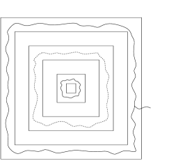
Figure 1: The event in the proof of Theorem 5 (in the case $k\geq m$ and $l<\infty$). The boxes, in order from smallest to largest, are $B(2^{k-m})$, $B(2^{k})$, $B(2^{k+l})$, $B(2^{k+l+m/4})$, $B(2^{k+l+m/2})$ and $B(2^{k+l+m})$. (Boxes are not drawn to scale.) The dotted path is $p_{2^{k+l+m/4}}$-closed, the path to infinity is $p_{2^{k+l+m/4}}$-open and the other two circuits are $p_{c}$-open. If all these paths exist, the sets ${\mathcal{S}}$ and ${\mathcal{G}}(k,l,m)$ coincide in $\operatorname{Ann}(2^{k},2^{k+l})$.

In the case that $k<m$ and $l<\infty$, we exclude condition (1) from the above argument. In the case $k<m$ and $l=\infty$ there is nothing to prove. If $k\geq m$ and $l=\infty$ we argue using only condition (1).

Remark 2.

Similar ideas were used in the proof of the upper bound in Theorem 1.4 in DS . Note that there is a typo there in the definition of $X^{n}_{i}$. It should be specified that $X^{n}_{i}$ counts only disconnecting edges with weights larger than $p_{c}$.

We now present corollaries of Theorem 5 that will help in the proofs of the next section. The first two are about mixing properties of the sequence $(X_{k})$. Recall the notation that $a_{k}=\mathbb{E}O_{k}$ and let $X_{k}=O_{k}-a_{k}$. For any $m_{1}\leq m_{2}$, let $\Sigma_{m_{1}}^{m_{2}}$ be the sigma algebra generated by the variables $X_{m_{1}},\ldots,X_{m_{2}}$. Write $\Sigma_{m_{1}}$ for $\lim_{m_{2}\to\infty}\Sigma_{m_{1}}^{m_{2}}$ and $\Sigma^{m_{2}}$ for $\Sigma_{1}^{m_{2}}$. For $m\geq 0$, define the strong mixing coefficient

$$\alpha(m)={\sup_{k\geq 1}}\sup_{A,B}|\mathbb{P}(A\cap B)-\mathbb{P}(A)\mathbb{P}(B)|,$$ (9)

where the supremum is over all $A\in\Sigma^{k}$ and $B\in\Sigma_{k+m}$.

Corollary 5

There exist constants $C<\infty$ and $\delta>0$ such that for all $m$,

$$\alpha(m)\leq C\exp(-\delta m).$$ (10)

Clearly it suffices to prove the corollary for $m>4$. Fix $k\geq 1$ and let $A\in\Sigma^{k}$, $B\in\Sigma_{k+m}$. For $j=1,\ldots,k$, let $\tilde{Y}_{j}$ be the number of outlets in $\mathcal{O}(0,k,\lfloor m/2\rfloor-1)\cap\operatorname{Ann}(2^{j-1},2^{j})$ with weight $>p_{c}$, and for $j\geq k+m$, let $\tilde{Y}_{j}$ be the number of outlets in $\mathcal{O}(k+m-1,\infty,\lfloor m/2\rfloor-1)\cap\operatorname{Ann}(2^{j-1},2^{j})$ with weight $>p_{c}$. Let $Y_{j}=\tilde{Y}_{j}-a_{j}$. By Theorem 5, there exist constants $C_{1}<\infty$ and $\delta_{1}>0$ such that for all $k\geq 1$, $m>4$,

$$\mathbb{P}(A_{k,m})\geq 1-C_{1}\exp(-\delta_{1}m),$$

where $A_{k,m}$ is the event that $X_{j}=Y_{j}$ for all $j\leq k$ and for all $j\geq k+m$.

Because $A\in\Sigma^{k}$, there exists a Borel set $A^{\prime}\subset{\mathbb{R}}^{k}$ such that $A$ is the event that $(X_{1},\ldots,X_{k})\in A^{\prime}$. Similarly, because $B\in\Sigma_{k+m}$, there exists a Borel set $B^{\prime}\subset{\mathbb{R}}^{\infty}$ (with the product topology) such that $B$ is the event that $(X_{k+m},\ldots)\in B^{\prime}$. Define $A_{Y}$ as the event that $(Y_{1},\ldots,Y_{k})\in A^{\prime}$ and $B_{Y}$ as the event that $(Y_{k+m},\ldots)\in B^{\prime}$. Because $A_{Y}$ and $B_{Y}$ are independent,

$$|\mathbb{P}(A_{Y}\cap B_{Y})-\mathbb{P}(A_{Y})\mathbb{P}(B_{Y})|=0.$$ (11)

Also, when $A_{k,m}$ occurs, the events $A$ and $A_{Y}$ (resp., $B$ and $B_{Y}$) are identical, so

$$|\mathbb{P}(A\cap B)-\mathbb{P}(A_{Y}\cap B_{Y})|\leq\mathbb{P}(A_{k,m}^{c})\leq C_{1}\exp(-\delta_{1}m)$$

and

$$|\mathbb{P}(A)\mathbb{P}(B)-\mathbb{P}(A_{Y})\mathbb{P}(B_{Y})| \leq \mathbb{P}(A)|\mathbb{P}(B)-\mathbb{P}(B_{Y})|$$

$${}+\mathbb{P}(B_{Y})|\mathbb{P}(A)-\mathbb{P}(A_{Y})|$$

$$\leq |\mathbb{P}(B)-\mathbb{P}(B_{Y})|+|\mathbb{P}(A)-\mathbb{P}(A_{Y})|$$

$$\leq 2C_{1}\exp(-\delta_{1}m).$$

Combining the two above inequalities with (11) gives the corollary.

Now that we have a bound on the decay of the sequence $(\alpha(m))$, we can relate this to the decay of covariances using the following classical result.

Corollary 6 ((Davydov , (2.2)))

Let $k,m\geq 1$ and let $f$ and $g$ be functions such that $f$ is $\Sigma^{k}$-measurable and $g$ is $\Sigma_{k+m}$-measurable. Suppose that $1/p+1/q<1$ and that the moments $\mathbb{E}|f|^{p}$ and $\mathbb{E}|g|^{q}$ exist. Then

$$|\mathbb{E}fg-\mathbb{E}f\mathbb{E}g|\leq 12[\mathbb{E}|f|^{p}]^{1/p}[\mathbb{E}|g|^{q}]^{1/q}[\alpha(m)]^{1-1/p-1/q}.$$ (12)

For completeness, we will outline the proof in the Appendix.

Corollaries 5 and 6 tell us that the variables $(X_{k})$ are very weakly dependent. This is one main ingredient for proving the CLT and SLLN for this sequence. In the first part of the following corollary, we will bound moments of the sums $(\sum_{k=1}^{n}X_{k})_{n}$. This is the second main ingredient necessary for proving the CLT. The second part of the corollary will control fluctuations of the sums and will be useful in proving the SLLN.

Corollary 7

The following statements hold. [(2)]

For each $0\leq t\leq 4$, there exists $D(t)<\infty$ such that for all $k\geq 1$ and $m\geq 0$,

$$\mathbb{E}\Biggl{|}\sum_{j=k}^{k+m}X_{j}\Biggr{|}^{t}\leq D(t)m^{t/2}.$$

There exists $C<\infty$ such that for any $\lambda>0$ and $n\geq 1$,

$$\mathbb{P}\Biggl{(}\max_{1\leq i\leq n}\Biggl{|}\sum_{k=1}^{i}X_{k}\Biggr{|}\geq\lambda\Biggr{)}\leq\frac{Cn}{\lambda^{2}}+\frac{C\sqrt{n}}{\lambda}.$$

We will begin with the proof of the first statement. It suffices to consider $t=4$ because for $t<4$ we can use Jensen’s inequality to reduce to this case. The statement will follow from Proposition 2.2 of Withers , which we state below as Lemma 1. For the statement, we need some definitions. For $0\leq k<n$, define

$$c^{(13)}(k,n)=\max_{1\leq x_{1},x_{2}=x_{1}+k\leq x_{3}\leq x_{4}\leq n}\mathbb{E}X_{x_{1}}X_{x_{2}}X_{x_{3}}X_{x_{4}}$$

and

$$c^{(31)}(k,n)=\max_{1\leq x_{1}\leq x_{2}\leq x_{3},x_{4}=x_{3}+k\leq n}\mathbb{E}X_{x_{1}}X_{x_{2}}X_{x_{3}}X_{x_{4}}.$$

Also set

$$c(k;1,3)=\sup_{n\geq k}\bigl{[}c^{(13)}(k,n)+c^{(31)}(k,n)\bigr{]}.$$

Lemma 1

Suppose that $\sup_{k\geq 1}\mathbb{E}X_{k}^{4}<\infty$ and

$$\sum_{k=0}^{m}(k+1)c(k;1,3)=O(m^{\gamma})\qquad\mbox{as }m\to\infty\mbox{ for }\gamma\geq 0.$$ (13)

Then

$$\sup_{b\geq 0}\mathbb{E}(X_{b}+\cdots+X_{b+a})^{4}=O(a^{2+\gamma})\qquad\mbox{as }a\to\infty.$$

We make the choice $\gamma=0$. The condition $\sup_{k\geq 1}\mathbb{E}X_{k}^{4}<\infty$ holds from Theorem 4. As for (13), it is not difficult to see that it will hold as long as we show that there exist constants $C_{1}<\infty$ and $\delta_{1}>0$ such that for any $m\geq 1$ and for any natural numbers $i_{1},\ldots,i_{4}$ such that the distance from $i_{1}$ to the set $\{i_{2},i_{3},i_{4}\}$ is at least equal to $m$,

$$|\mathbb{E}X_{i_{1}}\cdots X_{i_{4}}|\leq C_{1}\exp(-\delta_{1}m).$$ (14)

Condition (14) holds by Corollary 6. To show this, suppose that $i_{1}\leq i_{2}\leq i_{3}\leq i_{4}$ (the other cases are handled similarly). We make the choices $f=X_{i_{1}}$ and $g=X_{i_{2}}X_{i_{3}}X_{i_{4}}$, with $p=2$ and $q=4$. From Theorem 4, there exists $C_{2}$ such that for all $(i_{j})$, both $(\mathbb{E}g^{4})^{1/4}\leq C_{2}$ and $(\mathbb{E}f^{2})^{1/2}\leq C_{2}$. Since $\mathbb{E}f=0$, Corollary 6 gives

$$|\mathbb{E}X_{i_{1}}\cdots X_{i_{4}}|\leq C_{2}^{2}\alpha(m)^{1/4}.$$

Bounding $\alpha(m)$ using Corollary 5 shows (14) and completes the proof of the first statement of Corollary 7.

We now prove the second statement. It is the same as the proof of Lemma 2.2 in Davydov . Let $A_{n}$ be the event in the statement, and write $S_{n}=\sum_{k=1}^{n}X_{k}$. Let

$$A_{n}^{i}=\{|S_{j}|<\lambda\mbox{ for }j=1,\ldots,i-1\mbox{ but }|S_{i}|\geq\lambda\}.$$

Similarly to the proof of Kolmogorov’s maximal inequality for independent random variables, one can show that

$$\mathbb{P}(A_{n})\leq\frac{1}{\lambda^{2}}\Biggl{(}\mathbb{E}S_{n}^{2}+2\sum_{i=1}^{n}\mathbb{E}\bigl{[}I[A_{n}^{i}]S_{i}(S_{n}-S_{i})\bigr{]}\Biggr{)}.$$ (15)

By the first part of this corollary, $\mathbb{E}S_{n}^{2}\leq C_{3}n$. Next, write the summand as

$$\mathbb{E}\bigl{[}I[A_{n}^{i}]X_{i}(S_{n}-S_{i})\bigr{]}+\sum_{j=i+1}^{n}\mathbb{E}[I[A_{n}^{i}]S_{i-1}X_{j}].$$

The absolute value of the first term is bounded by

$$\Biggl{|}\sum_{k=i+1}^{n}\mathbb{E}[I[A_{n}^{i}]X_{i}X_{k}]\Biggr{|}\leq\sum_{k=i+1}^{n}C_{4}[\alpha(k-i)]^{1/4}\leq C_{5},$$

where we use Corollary 6 with $f=I[A_{n}^{i}]X_{i}$ and $g=X_{k}$, with $p=2$ and $q=4$ (bounding the moments using Theorem 4) in the first inequality. For the second term we also use Corollary 6 but choose $f=I[A_{n}^{i}]S_{i-1}$ and $g=X_{j}$, with $p=2$ and $q=4$. This produces the bound

$$C_{6}\sum_{j=i+1}^{n}(\mathbb{E}[S_{i-1}I[A_{n}^{i}]]^{2})^{1/2}[\alpha(j-i)]^{1/4} \leq C_{6}\lambda\sqrt{\mathbb{P}(A_{n}^{i})}\sum_{j=1}^{\infty}[\alpha(j)]^{1/4}$$

$$\leq C_{7}\lambda\sqrt{\mathbb{P}(A_{n}^{i})}.$$

Summing over $i$ and using Jensen’s inequality with the square root function (recalling that the events $A_{n}^{i}$ are disjoint in $i$), we see that the sum in (15) is no bigger than

$$2C_{5}n+2C_{7}\lambda n\Biggl{(}\frac{1}{n}\sum_{i=1}^{n}\sqrt{\mathbb{P}(A_{n}^{i})}\Biggr{)}\leq C_{8}n+C_{9}\lambda\sqrt{n}.$$

Putting both this bound and the one on $\mathbb{E}S_{n}^{2}$ into (15) finishes the proof.

The following corollary shows a way to construct a sequence of $c\log n$-dependent random variables $(\tilde{O}_{k})$ related to $(O_{k})$. We will not use this sequence in the rest of the paper; however, the proofs of the CLT and the SLLN given in Section 4 can be replaced by ones that make reference to neither Davydov nor Withers but that come from corresponding statements involving independent random variables by using the $\tilde{O}_{k}$’s. An example of such an approach is the proof of Theorem 1.4 in DS .

Corollary 8

For any $\gamma>0$, there exists $c<\infty$ such that for all $n\geq 1$, defining $m_{n}=c\log n$, with probability at least $1-cn^{-\gamma}$, all random variables $O_{m_{n}+1},\ldots,O_{n}$ are equal to some random variables $\tilde{O}_{m_{n}+1},\ldots,\tilde{O}_{n}$, which are $m_{n}$-dependent and satisfy Theorem 4.

Let $c$ be an integer to be chosen later and let $k\geq c\log n$. We define $\tilde{O}_{k}$ as the number of outlets in $\mathcal{O}(k-1,1,\lfloor m_{n}/2\rfloor-1)\cap\operatorname{Ann}(2^{k-1},2^{k})$ with $\mathrm{weight}>p_{c}$. The reader may verify that exactly the same argument used in DS for the proof of Theorem 4 applies to each $\tilde{O}_{k}$. Also, the variables $(\tilde{O}_{k})$ are obviously $m_{n}$-dependent. By Theorem 5, there exist $C<\infty$ and $\beta>0$ such that for any $k\geq c\log n$,

$${\mathbb{P}}(\tilde{O}_{k}\neq O_{k})\leq Cn^{-\beta},$$

where $\beta\to\infty$ as $c\to\infty$. Therefore,

$${\mathbb{P}}(\tilde{O}_{k}\neq O_{k}\mbox{ for some }k\in[c\log n,n])\leq Cn^{1-\beta}.$$

4 CLT and SLLN for the outlets

4.1 Proof of Theorem 1

First we will show the statement about the $a_{k}$’s. Theorem 4 implies the upper bound on $a_{k}$, so we need only show the lower bound. The proof is similar to the first part of Theorem 1.4 in DS . For $k\geq 1$, let $A_{k}$ be the event that (a) there is a $p_{2^{k}}$-closed circuit around the origin in $\operatorname{Ann}(2^{k-1},2^{k})$, (b) there is a $p_{2^{k}}$-open circuit in $\operatorname{Ann}(2^{k-1},2^{k})$ and (c) the circuit from (b) is connected by a $p_{2^{k}}$-open path to infinity. By the RSW theorem and (5), there exists $C_{1}>0$ such that for all $k$,

$$\mathbb{P}(A_{k})>C_{1}.$$

But $A_{k}$ implies the event $\{O_{k}\geq 1\}$, so

$$a_{k}=\mathbb{E}O_{k}\geq\mathbb{P}(A_{k})\geq C_{1}.$$

We move on to the statement about $b(n)$. The upper bound follows from the case $t=2$ of the first statement in Corollary 7, so we will focus on the lower bound. Let $k$ be an integer between 1 and $n$ and let $L_{n}:=\log n$. For $i=1,\ldots,5$ define $q_{k}(i)=p_{c}+i(p_{2^{k}}-p_{c})$. We define $A_{n,k}$ as the event that: [(2)]

there is an edge $e_{1}$ in $\operatorname{Ann}(2^{k+1},2^{k+2})$, with weight between $q_{k}(4)$ and $q_{k}(5)$, which is connected by a $p_{c}$-open path to a $p_{c}$-open circuit around the origin that is in $\operatorname{Ann}(2^{k},2^{k+1})$;

the endpoints of $e_{1}^{*}$ are connected by a $q_{k}(5)$-closed dual path in $\operatorname{Ann}(2^{k+1}$, $2^{k+2})^{*}$ such that the union of this path and $e_{1}^{*}$ encloses the origin;

there is an edge $e_{2}$ in $\operatorname{Ann}(2^{k+2},2^{k+3})$, with weight in $[q_{k}(1),q_{k}(2)]\cup[q_{k}(3),q_{k}(4)]$, which is connected by a $p_{c}$-open path to an endpoint of $e_{1}$;

the endpoints of $e_{2}^{*}$ are connected by a $q_{k}(5)$-closed dual path in $\operatorname{Ann}(2^{k+2}$, $2^{k+3})^{*}$ such that the union of this path and $e_{2}^{*}$ encloses the origin;

there is an edge $e_{3}$ in $\operatorname{Ann}(2^{k+3},2^{k+4})$ with weight in $[q_{k}(2),q_{k}(3)]$, which is connected by a $p_{c}$-open path to an endpoint of $e_{2}$;

the endpoints of $e_{3}^{*}$ are connected by a $q_{k}(5)$-closed dual path in $\operatorname{Ann}(2^{k+3}$, $2^{k+4})^{*}$ such that the union of this path and $e_{3}^{*}$ encloses the origin;

an endpoint of $e_{3}$ is connected by a $q_{k}(1)$-open path to $\partial B(2^{k+L_{n}})$. Notice that if $A_{n,k}$ occurs with edges $e_{1}-e_{3}$, it cannot occur with any other edges. It follows from DSV , Lemma 6.3, and RSW arguments (similar to the proof of DSV , Corollary 6.2) that there exists $C_{2}>0$ such that for any $n,k,$

$$\mathbb{P}(A_{n,k})\geq C_{2}.$$ (16)

Since, in addition, the events $A_{n,k}$ are $L_{n}$-dependent for fixed $n$, there exists $C_{3}>0$ such that

$$\mathbb{P}(A_{n,3k}\mbox{ occurs for at least }C_{3}n\mbox{ values of }k\in[1,n/3])\to 1$$ (18)

$$\eqntext{\mbox{as }n\to\infty.}$$

To see this, we will give the proof in Theorem 1.4 of DS . Let $j$ be an integer between 1 and $L_{n}$, and define $B_{i}^{j}=A_{n,3(j+iL_{n})}$. Note that the events $(B_{i}^{j})_{i=0}^{\lfloor n/3L_{n}\rfloor-1}$ are independent. Therefore we may use Lemma 5.2 from DS . Its proof is standard, so we omit it.

Lemma 2

Let $c>0$. There exist $\alpha>0$ and $\beta<1$ depending on $c$ with the following property. If $Y_{i}$ are independent $0/1$ random variables (not necessarily identically distributed) with $\mathbb{P}(Y_{i}=1)>c$ for all $i$, then for all $n$,

$$\mathbb{P}\Biggl{(}\sum_{i=1}^{n}Y_{i}<\alpha n\Biggr{)}<\beta^{n}.$$

In view of this lemma and (16), there exist $\alpha>0$ and $\beta<1$ such that for any $n$ and $1\leq j\leq L_{n}$,

$$\mathbb{P}\Biggl{(}\sum_{i=0}^{\lfloor n/3L_{n}\rfloor-1}I[B_{i}^{j}]<\frac{\alpha n}{3L_{n}}\Biggr{)}<\beta^{n/3L_{n}}.$$

Therefore,

$$\mathbb{P}\Biggl{(}\sum_{j=1}^{L_{n}}\sum_{i=0}^{\lfloor n/3L_{n}\rfloor-1}I[B_{i}^{j}]<\alpha n/3\Biggr{)}$$

$$\qquad\leq\mathbb{P}\Biggl{(}\sum_{i=0}^{\lfloor n/3L_{n}\rfloor-1}I[B_{i}^{j}]<\alpha n/3L_{n}\mbox{ for some }j\in[1,L_{n}]\Biggr{)}$$

$$\qquad\leq L_{n}\beta^{n/3L_{n}},$$

which converges to 0 as $n\to\infty$. This proves (18).

Define $\tilde{A}_{n,k}$ the same way as we defined $A_{n,k}$ except that in item 7, the $q_{k}(1)$-open path connects $e_{3}$ to infinity. (See Figure 2 for an illustration of the event $\tilde{A}_{n,k}$.) Note that if $\tilde{A}_{n,k}$ occurs, then $e_{1}$ and $e_{3}$

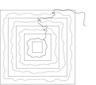
Figure 2: The event $\tilde{A}_{n,k}$. The boxes, in order from smallest to largest, are $B(2^{k+i})$ for $i=0,\ldots,4$. The dotted paths are $q_{k}(5)$-closed, the path from $e_{3}$ to infinity is $q_{k}(1)$-open and all the other paths are $p_{c}$-open. The weight of $e_{1}$ is in $[q_{k}(4),q_{k}(5)]$, the weight of $e_{3}$ is in $[q_{k}(2),q_{k}(3)]$ and the weight of $e_{2}$ is in $[q_{k}(1),q_{k}(2)]\cup[q_{k}(3),q_{k}(4)]$. The edges $e_{1}$ and $e_{3}$ are outlets. The edge $e_{2}$ is an outlet if and only if its weight is in $[q_{k}(3),q_{k}(4)]$.

are outlets, and $e_{2}$ is an outlet if and only if its weight is in $[q_{k}(3),q_{k}(4)]$. If $A_{n,k}$ occurs but $\tilde{A}_{n,k}$ does not, then there exists a $q_{k}(1)$-closed dual circuit around the origin with radius at least $2^{k+L_{n}}$. By (6), there exist constants $C_{4}<\infty$ and $C_{5}>0$ such that for all $n,k$, $\mathbb{P}(A_{n,k}\setminus\tilde{A}_{n,k})\leq C_{4}\exp(-C_{5}2^{k+L_{n}}/2^{k})$, so

$$\mathbb{P}(A_{n,k}\setminus\tilde{A}_{n,k}\mbox{ occurs for some }k\in[1,n])\to 0.$$

Therefore we may find $C_{6}>0$ such that for all $n$,

$$\mathbb{P}(\tilde{A}_{n,3k}\mbox{ occurs for at least }C_{3}n\mbox{ values of }k\in[1,n/3])>C_{6}.$$

Call $A$ the above event whose probability is bounded below by $C_{6}$. On the event $A$, we define the vector $\vec{f}=(f_{1},\ldots,f_{\lfloor C_{3}n\rfloor})$ whose entries are the first $\lfloor C_{3}n\rfloor$ edges $e$ (ordered from distance to the origin) such that there exist edges $\bar{e}_{1}$ and $\bar{e}_{3}$ such that $\bar{e}_{1}$, $e$ and $\bar{e}_{3}$ satisfy the properties of $e_{1},e_{2}$ and $e_{3}$, respectively, in the definition of $A_{n,3k}$ for some $k\in[1,n/3]$. Write $O_{\vec{f}}(n)$ for the number of outlets that appear in the vector $\vec{f}$, and write $U_{\vec{f}}$ for the number of outlets in $B(2^{n})$ that do not appear in $\vec{f}$. At least one of $\{U_{\vec{f}}+(C_{2}n)/2\geq a(n)\}$ or $\{U_{\vec{f}}+(C_{2}n)/2\leq a(n)\}$ has probability at least $C_{6}/3$. Let us assume that it is the first event; if it is the other then the subsequent argument can be easily modified. Write $B=\{U_{\vec{f}}+(C_{2}n)/2\geq a(n)\}$. Since $U_{\vec{f}}$ is defined only on $A$, we have $B\subset A$.

Associated to each $f_{k}$ in $\vec{f}$ in the definition of $A_{n,k}$ are two intervals $I_{k}(1)=[q_{k}(1),q_{k}(2)]$ and $I_{k}(2)=[q_{k}(3),q_{k}(4)]$. Let $\eta(\vec{f})$ be the configuration of weights outside of $\vec{f}$. If $\vec{f}$ and $\eta(\vec{f})$ are fixed, then the variable $U_{\vec{f}}$ is a constant function of the weights $\tau_{f_{k}}$. Also, when these variables are fixed, $O_{\vec{f}}(n)$ is equal to the number of values of $k\in[1,\lfloor C_{3}n\rfloor]$ such that $\tau_{f_{k}}\in I_{k}(2)$. Since the lengths of $I_{k}(1)$ and $I_{k}(2)$ are equal, the distribution of $O_{\vec{f}}(n)$ conditioned on $\vec{f}$, $\eta(\vec{f})$ and $B$ is Binomial$(\lfloor C_{3}n\rfloor,1/2)$. If $Y$ is an independent variable with this distribution, then

$$\mathbb{P}\bigl{(}|{\mathbf{O}}(n)-a_{n}|\geq\sqrt{n}\bigr{)} \geq \mathbb{E}\bigl{[}\mathbb{P}\bigl{(}O_{\vec{f}}(n)\geq(C_{3}n)/2+\sqrt{n}\mid B,\vec{f},\eta(\vec{f})\bigr{)}\bigr{]}\mathbb{P}(B)$$

$$\geq (C_{6}/3)\mathbb{P}\bigl{(}Y\geq(C_{3}n)/2+\sqrt{n}\bigr{)},$$

which is bounded below uniformly in $n$. This completes the proof.

4.2 Proof of Theorem 2

Proof of the CLT We will apply Theorem 2.1 of Withers . To state that theorem, we need to introduce the notion of $l$-mixing. For $k\geq 0$, $n\geq 1$ and $u\in{\mathbb{R}}$, set

$$l_{n}(k,u)=\max_{1\leq j\leq n-k}\sup|\mathbb{E}[e^{iuP}e^{-iuF}]-\mathbb{E}e^{iuP}\mathbb{E}e^{-iuF}|,$$ (19)

where

$$P=b(n)^{-1}\sum_{l=1}^{j}\delta_{l}X_{l},\qquad F=b(n)^{-1}\sum_{l=j+k}^{n}\delta_{l}X_{l},$$

and the supremum in (19) is over all $\{\delta_{l}=0\mbox{ or }1\}$. Now for $k\geq 0$ and $u\in{\mathbb{R}}$, set

$$l(k,u)=\sup_{n\geq 1}l_{n}(k,u).$$

The sequence $(X_{k})$ is called $l$-mixing if for all real $u$, $l(k,u)\to 0$ as $k\to\infty$.

Remark 3.

As mentioned in the discussion below Definition 2.2 in Withers , the inequality

$$l(k,u)\leq 16\alpha(k)$$ (20)

from page 307 in IL holds for all $k\geq 0$ and $u\in{\mathbb{R}}$, so since $\alpha(k)\to 0$ as $k\to\infty$, the sequence $(X_{k})$ of outlet variables is $l$-mixing.

For $k\geq 0$, define

$$\tilde{c}(k)=\sup_{j\geq 1}|\mathbb{E}X_{j}X_{j+k}|.$$

The following is Theorem 2.1 of Withers .

Lemma 3

The following conditions are sufficient for

$$\frac{\sum_{k=1}^{n}X_{k}}{b(n)}\Rightarrow N(0,1).$$

For some $\varepsilon>0$ and $\gamma\geq 0$,

$$\sup_{a\geq 1}\mathbb{E}\Biggl{|}\sum_{k=a}^{a+b}X_{k}\Biggr{|}^{2+\varepsilon}=O(b^{1+\varepsilon/2+\gamma})\qquad\mbox{as }b\to\infty;$$ (21)

the sequence $(X_{k})$ is $l$-mixing and for all real $u$,

$$l(k,u)=o(k^{-\theta})\qquad\mbox{as }k\to\infty,\mbox{ where }\theta=2\gamma/\varepsilon,$$ (22)

and

$$b(n)\to\infty\qquad\mbox{as }n\to\infty\quad\mbox{and}\quad\sum_{j=0}^{\infty}\tilde{c}(j)<\infty.$$ (23)

To prove the CLT, we simply need to verify the conditions of Lemma 3. Condition (21) holds with $\varepsilon=2$ and $\gamma=0$ by the first part of Corollary 7, using $t=4$. Using (20) and Corollary 5, we see that condition (22) holds. Also, the first part of Corollary 7 with $t=2$ shows the first part of condition (23). Finally, to verify the second part of (23), we appeal to Corollary 6 using $f=X_{m}$ and $g=X_{m+k}$ (for fixed $m\geq 1$ and $k\geq 0$), with $p=2$ and $q=4$. It follows that

$$\tilde{c}(k)\leq C_{1}\alpha(k)^{1/4}$$

for some $C_{1}<\infty$. In view of Corollary 5, this proves the second part of (23) and completes the proof of the CLT. Proof of the SLLN For $i\geq 1$, take $n_{i}=2^{i}$. The second statement of Corollary 7 implies that for any $\varepsilon>0$,

$$\mathbb{P}\Bigl{(}{\max_{n_{i}\leq j\leq n_{i+1}}}|{\mathbf{O}}(j)-a(j)|\geq\varepsilon n_{i}^{r}\Bigr{)} \leq \frac{C}{\varepsilon^{2}}\biggl{(}\frac{n_{i+1}}{n_{i}^{2r}}+\frac{\sqrt{n_{i+1}}}{n_{i}}\biggr{)}$$

$$\leq C_{1}\biggl{(}\frac{1}{(2^{2r-1})^{i}}+\frac{1}{(2^{r-1/2})^{i}}\biggr{)}.$$

Since $r>1/2$, this probability is summable in $i$. Since the function $n^{r}$ is monotone, it follows that

$$\sum_{i=1}^{\infty}\mathbb{P}\biggl{(}\max_{n_{i}\leq j\leq n_{i+1}}\frac{|{\mathbf{O}}(j)-a(j)|}{j^{r}}\geq\varepsilon\biggr{)}<\infty.$$

The Borel–Cantelli lemma finishes the proof.

5 Further results for invasion percolation

We begin with a lemma.

Lemma 4

There exist constants $C<\infty$ and $\alpha>0$ such that for all $m,n\geq 1$,

$$\mathbb{P}\bigl{(}{\mathbf{O}}(n,n+m)\leq\alpha m\bigr{)}\leq C\exp(-m^{\alpha}),$$

where ${\mathbf{O}}(n,n+m)$ is the number of outlets in $\operatorname{Ann}(2^{n},2^{n+m})$.

The proof of the lower bound in Theorem 1.4 of DS shows the case $n=1$. For general $n$ the proof is similar. For $i,m\geq 1$, let $G_{i,m}$ be the event that there is no $p_{2^{i}}$-closed dual circuit around the origin with radius larger than $2^{i+\log m}$, and let $K_{i,m}$ be the event that (a) there exists a $p_{2^{i}}$-closed dual circuit ${\mathcal{C}}$ around the origin in $\operatorname{Ann}(2^{i},2^{i+1})^{*}$, (b) there exists a $p_{c}$-open circuit ${\mathcal{C}}^{\prime}$ around the origin in $\operatorname{Ann}(2^{i},2^{i+1})$ and (c) the circuit ${\mathcal{C}}^{\prime}$ is connected to $\partial B(2^{i+\log m})$ by a $p_{2^{i}}$-open path. By the RSW theorem and (5), there exists $C_{1}>0$ such that for all $i\geq 0$ and $m\geq 1$,

$$\mathbb{P}(K_{i,m})\geq C_{1}.$$

Now let $j$ be an integer between $1$ and $\log m$, and define the event $K_{i,m}^{j}=K_{n+j+i\lfloor\log m\rfloor,m}$. Note that for fixed $j$, the events $(K_{i,m}^{j})_{i=0}^{\lfloor m/\log m\rfloor-1}$ are independent. Therefore we can apply Lemma 2 to deduce that there exist $\alpha_{0}>0$ and $\beta_{0}<1$ such that for any $m,n$ and $1\leq j\leq\log m$,

$$\mathbb{P}\Biggl{(}\sum_{i=0}^{\lfloor m/\log m\rfloor-1}I[K_{i,m}^{j}]<\frac{\alpha_{0}m}{\lfloor\log m\rfloor}\Biggr{)}<\beta_{0}^{m/\log m}.$$

Therefore,

$$\mathbb{P}\Biggl{(}\sum_{j=1}^{\lfloor\log m\rfloor}\sum_{i=0}^{\lfloor m/\log m\rfloor-1}I[K_{i,m}^{j}]<\alpha_{0}m\Biggr{)}$$

$$\qquad\leq\mathbb{P}\Biggl{(}\sum_{i=0}^{\lfloor m/\log m\rfloor-1}I[K_{i,m}^{j}]<\alpha_{0}m/\lfloor\log m\rfloor\mbox{ for some }j\in[1,\log m]\Biggr{)}$$

$$\qquad\leq\log m\beta_{0}^{m/\log m}\leq C_{2}\exp(-m^{\alpha})$$

for some $C_{2}<\infty$ and $\alpha>0$. By (6), we also have the estimate

$$\sum_{i=0}^{m}\mathbb{P}(G_{n+i,m}^{c})\leq C_{3}\sum_{i=0}^{m}\exp(-C_{4}m)\leq C_{3}\exp(-C_{5}m).$$

Since the event $K_{i,m}\cap G_{i,m}$ implies $O_{i+1}\geq 1$, we can combine the above estimates to deduce

$$\mathbb{P}\bigl{(}{\mathbf{O}}(n,n+m)\leq\alpha_{0}m\bigr{)}\leq C_{2}\exp(-m^{\alpha})+C_{3}\exp(-C_{5}m),$$

which implies the lemma.

Recall the definitions of $Q_{n}$ and $T_{n}$ from Section 1.3. Since $a(n)\asymp n$, $T_{n}$ is comparable with $n$. Proof of Theorem 3 It follows from the definition of $Q_{n}$, the CLT for ${\mathbf{O}}(n)$ and the fact that for any $x$, $\sigma_{n+x\sqrt{n}}/\sigma_{n}\to 1$ as $n\to\infty$ that

$${\mathbb{P}}(Q_{n}<T_{n+x\sigma_{n}})\to\Phi(x),$$

where $\Phi$ is the standard normal cumulative distribution function. Recall that the $a_{i}$’s [$a_{i}=a(i)-a(i-1)$] are uniformly bounded away from 0 and $\infty$ by Theorem 1. Therefore,

$${\mathbb{P}}(Q_{n}<T_{n+x\sigma_{n}})={\mathbb{P}}\bigl{(}a(Q_{n})<a(T_{n+x\sigma_{n}})\bigr{)}={\mathbb{P}}\bigl{(}a(Q_{n})<n+x\sigma_{n}+r_{n}\bigr{)},$$

where $r_{n}$ is uniformly bounded in $n$. It remains to prove the second part of the proposition. The first statement implies that for any $M>0$,

$${\mathbb{E}}\min\biggl{\{}\biggl{(}\frac{a(Q_{n})-n}{\sigma_{n}}\biggr{)}^{2},M\biggr{\}}\to{\mathbb{E}}\min\{Z^{2},M\},$$

where $Z$ is a standard normal random variable. Therefore, it suffices to show that for any $\varepsilon>0$ there exists $C_{1}>0$ such that

$$\limsup_{n\to\infty}{\mathbb{E}}\biggl{(}\frac{a(Q_{n})-n}{\sigma_{n}}\biggr{)}^{2}I\bigl{(}|a(Q_{n})-n|>C_{1}\sigma_{n}\bigr{)}<\varepsilon.$$

This will follow if we show that there exists $C_{2}$ such that for all $n$,

$${\mathbb{E}}\biggl{(}\frac{a(Q_{n})-n}{\sigma_{n}}\biggr{)}^{4}<C_{2}.$$

In other words, we need to show that ${\mathbb{E}}(a(Q_{n})-n)^{4}=O(n^{2})$. Since the $a_{i}$’s are uniformly bounded away from 0 and $\infty$, it suffices to show that ${\mathbb{E}}(Q_{n}-T_{n})^{4}=O(n^{2})$. For $c>0$, consider

$$A_{n}=\bigl{\{}{\mathbf{O}}(n,n+k)>ck,{\mathbf{O}}(n-k,n)>ck\mbox{ for all }k\geq\sqrt{n}\bigr{\}}.$$

It follows from Lemma 4 that there exists $c>0$ such that

$${\mathbb{P}}(A_{n}^{c})\leq C_{3}\exp(-n^{c}).$$

We write

$${\mathbb{E}}(Q_{n}-T_{n})^{4}={\mathbb{E}}(Q_{n}-T_{n})^{4}I(Q_{n}\leq C_{4}n)+{\mathbb{E}}(Q_{n}-T_{n})^{4}I(Q_{n}>C_{4}n).$$

If $C_{4}$ is large enough, ${\mathbb{E}}(Q_{n}-T_{n})^{4}I(Q_{n}>C_{4}n)=o(n^{2})$ (One can write $I(Q_{n}>C_{4}n)$ as $\sum_{k=1}^{\infty}I(Q_{n}\in(kC_{4}n,(k+1)C_{4}n])$ and use Lemma 4). We now bound the first expectation.

$${\mathbb{E}}(Q_{n}-T_{n})^{4}I(Q_{n}\leq C_{4}n)$$

$$\qquad\leq(C_{4}n)^{4}{\mathbb{P}}(A_{T_{n}}^{c})+T_{n}^{2}+{\mathbb{E}}(Q_{n}-T_{n})^{4}I\bigl{(}|Q_{n}-T_{n}|>\sqrt{T_{n}},A_{T_{n}}\bigr{)}.$$

The first two summands are bounded by $C_{5}n^{2}$. It remains to bound the last summand

$${\mathbb{E}}(Q_{n}-T_{n})^{4}I\bigl{(}Q_{n}-T_{n}>\sqrt{T_{n}},A_{T_{n}}\bigr{)}$$

$$\qquad\leq{\mathbb{E}}(Q_{n}-T_{n})^{4}I\bigl{(}Q_{n}>T_{n},{\mathbf{O}}(T_{n},Q_{n}-1)>c(Q_{n}-1-T_{n})\bigr{)}$$

$$\qquad\leq\frac{8}{c^{4}}{\mathbb{E}}\bigl{(}{\mathbf{O}}(Q_{n}-1)-{\mathbf{O}}(T_{n})\bigr{)}^{4}I(Q_{n}>T_{n})+8$$

$$\qquad\leq\frac{8}{c^{4}}{\mathbb{E}}\bigl{(}{\mathbf{O}}(T_{n})-n\bigr{)}^{4}+8$$

$$\qquad\leq C_{6}n^{2},$$

where the last inequality follows from Corollary 7. Similarly, one can show that ${\mathbb{E}}(Q_{n}-T_{n})^{4}I(Q_{n}-T_{n}<-\sqrt{T_{n}},A_{T_{n}})\leq C_{7}n^{2}$. Proof of Corollary 1 It follows from Theorem 1 that $a(T_{n})=n+O(1)$, $\sigma_{n}\asymp\sqrt{n}$ and $|a(m)-a(n)|\asymp|m-n|$ independently of $m,n$. Therefore, the first statement of Corollary 1 follows directly from Theorem 3. The upper bound in the second statement follows immediately from the upper bound in the first statement. For the lower bound, we may apply the CLT for $(a(Q_{n}))$ to deduce that there exists $C>0$ such that for all $n$,

$$\mathbb{P}\bigl{(}Q_{n}\geq T_{n}+\sqrt{n}\bigr{)}>C\quad\mbox{and}\quad\mathbb{P}\bigl{(}Q_{n}\leq T_{n}-\sqrt{n}\bigr{)}>C.$$

The lower bound follows from these two estimates. Indeed, if $\mathbb{E}Q_{n}\geq T_{n}$, then $Q_{n}\leq T_{n}-\sqrt{n}$ implies that $Q_{n}\leq\mathbb{E}Q_{n}-\sqrt{n}$ and so

$$\mathbb{E}(Q_{n}-\mathbb{E}Q_{n})^{2}\geq n\mathbb{P}\bigl{(}Q_{n}\leq T_{n}-\sqrt{n}\bigr{)}>Cn.$$

If $\mathbb{E}Q_{n}\leq T_{n}$, then the argument is similar. Proof of Corollary 2 The proofs of both statements are similar so we only show the proof of the first. We first prove the lower bound. The CLT for $(a(Q_{n}))$ implies that there exists $C_{1}$ such ${\mathbb{P}}(Q_{n}>T_{n}+\sqrt{n})>C_{1}$. It is obvious that $\hat{R}_{n}\geq 2^{Q_{n}-1}$. Therefore, ${\mathbb{P}}(\hat{R}_{n}\geq 2^{T_{n}+\sqrt{n}-1})>C_{1}$, which implies that ${\mathbb{E}}(\log\hat{R}_{n}-T_{n})^{2}\geq(\sqrt{n}-1)^{2}C_{1}$.

We now prove the upper bound. We first observe that by Theorem 4, using $t=4$,

$$\mathbb{P}\bigl{(}\hat{R}_{n}<2^{\sqrt{n}}\bigr{)} \leq \mathbb{P}\bigl{(}Q_{n}\leq\sqrt{n}\bigr{)}\leq\mathbb{P}\bigl{(}{\mathbf{O}}\bigl{(}\sqrt{n}\bigr{)}\geq n\bigr{)}$$

$$\leq \mathbb{E}\mathbf{O}\bigl{(}\sqrt{n}\bigr{)}^{4}/n^{4}=O(n^{-2}).$$

Therefore, ${\mathbb{E}}(\log\hat{R}_{n}-T_{n})^{2}I(\hat{R}_{n}<2^{\sqrt{n}})=o(n)$. We next rule out the case when $\hat{R}_{n}>2^{C_{2}n}$ for large enough $C_{2}$.

$${\mathbb{E}}(\log\hat{R}_{n}-T_{n})^{2}I(\hat{R}_{n}>2^{C_{2}n}) \leq {\mathbb{E}}(\log\hat{R}_{n})^{2}I(\hat{R}_{n}>2^{C_{2}n})$$

$$\leq \sum_{k=1}^{\infty}\bigl{(}C_{2}n(k+1)\bigr{)}^{2}{\mathbb{P}}(\hat{R}_{n}>2^{C_{2}nk}).$$

Note that ${\mathbb{P}}(\hat{R}_{n}>2^{C_{2}nk})$ is bounded above by

$${\mathbb{P}}\bigl{(}\mbox{there is no }p_{c}\mbox{-open circuit around the origin in }\operatorname{Ann}\bigl{(}2^{C_{2}nk-\sqrt{C_{2}nk}},2^{C_{2}nk}\bigr{)}\bigr{)}$$

$$\qquad{}+{\mathbb{P}}\bigl{(}Q_{n}>C_{2}nk-\sqrt{C_{2}nk}\bigr{)}.$$

Using the RSW theorem and Lemma 4 if $C_{2}$ is large enough, this gives the bound

$${\mathbb{P}}(\hat{R}_{n}>2^{C_{2}nk})\leq C_{3}\exp(-(nk)^{C_{4}}).$$ (25)

Therefore,

$${\mathbb{E}}(\log\hat{R}_{n}-T_{n})^{2}I(\hat{R}_{n}>2^{C_{2}n})=o(n).$$

Let $\tilde{A}_{n}$ be the event that there exists a $p_{c}$-open circuit around the origin in $\operatorname{Ann}(2^{k-\sqrt{k}},2^{k})$ for all $k\geq\sqrt{n}$. It follows from the RSW theorem that

$${\mathbb{P}}(\tilde{A}_{n}^{c})\leq C_{5}\exp(-n^{C_{6}}).$$ (26)

Therefore,

$${\mathbb{E}}(\log\hat{R}_{n}-T_{n})^{2}I(\hat{R}_{n}\leq 2^{C_{2}n},\tilde{A}_{n}^{c})=o(n).$$

Moreover, if $\hat{R}_{n}>2^{\sqrt{n}}$ and $\tilde{A}_{n}$ occurs, then $Q_{n}\geq\log\hat{R}_{n}-\sqrt{\log\hat{R}_{n}}-1$. Hence

$${\mathbb{E}}(\log\hat{R}_{n}-T_{n})^{2}I\bigl{(}2^{\sqrt{n}}\leq\hat{R}_{n}\leq 2^{C_{2}n},\tilde{A}_{n}\bigr{)}$$

$$\qquad\leq 2{\mathbb{E}}(Q_{n}-T_{n})^{2}+2{\mathbb{E}}(\log\hat{R}_{n}-Q_{n})^{2}I\bigl{(}Q_{n}>\log\hat{R}_{n}-\sqrt{C_{2}n}-1\bigr{)}$$

$$\qquad\leq C_{7}n.$$

The last inequality follows from Corollary 1 and from the fact that $Q_{n}\leq\log\hat{R}_{n}+1$. The upper bound is proved. Proof of Corollary 3 For any $n$, let

$$f(n)=\max\{\tau_{e}\dvtx e\mbox{ is an outlet in }B(n)^{c}\}$$

and $g(n)=\min\{\tau_{e}\dvtx e$ is an outlet in $B(n)\}$ if there is an outlet in $B(n)$ and $g(n)=0$ otherwise.

Lemma 5

There exists $C<\infty$ such that for any $t\geq 1$ and $n\geq 1$,

$${\mathbb{E}}\biggl{(}\biggl{|}\log\frac{f(n)-p_{c}}{p_{n}-p_{c}}\biggr{|}^{t}\biggr{)}\leq(Ct)^{Ct}\quad\mbox{and}\quad{\mathbb{E}}\biggl{(}\biggl{|}\log\frac{g(n)-p_{c}}{p_{n}-p_{c}}\biggr{|}^{t}\biggr{)}\leq(Ct)^{Ct}.$$

Using the RSW theorem and (6), respectively, we see that there exist constants $C_{1}<\infty$ and $C_{2}>0$ such that for any $n\geq 1$ and $p\in(0,1)$,

$${\mathbb{P}}\bigl{(}f(n)<p\bigr{)}\leq{\mathbb{P}}\bigl{(}B(n)\stackrel{{\scriptstyle p}}{{\leftrightarrow}}\infty\bigr{)}\leq C_{1}\biggl{(}\frac{n}{L(p)}\biggr{)}^{C_{2}}$$

and

$${\mathbb{P}}\bigl{(}f(n)\geq p\bigr{)}\leq{\mathbb{P}}(B_{n,p})\leq C_{1}\exp\biggl{(}-C_{2}\frac{n}{L(p)}\biggr{)},$$

where $B_{n,p}$ is defined directly above (6). For $k\in{\mathbb{Z}}$, let $q_{k}=p_{2^{k}n}$

$${\mathbb{E}}\biggl{(}\biggl{|}\log\frac{f(n)-p_{c}}{p_{n}-p_{c}}\biggr{|}^{t}\biggr{)}$$

$$\qquad=\sum_{k}{\mathbb{E}}\biggl{(}\biggl{|}\log\frac{f(n)-p_{c}}{p_{n}-p_{c}}\biggr{|}^{t}I\bigl{(}f(n)\in[q_{k+1},q_{k})\bigr{)}\biggr{)}$$

$$\qquad\leq\sum_{k\geq 0}\biggl{|}\log\frac{q_{k+1}-p_{c}}{p_{n}-p_{c}}\biggr{|}^{t}{\mathbb{P}}\bigl{(}f(n)<q_{k}\bigr{)}$$

$$\qquad\quad{}+\sum_{k<0}\biggl{|}\log\frac{q_{k}-p_{c}}{p_{n}-p_{c}}\biggr{|}^{t}{\mathbb{P}}\bigl{(}f(n)\geq q_{k+1}\bigr{)}.$$

The first result of the lemma follows from (7) and the above estimates. It remains to prove the second statement. Note that for any $n\geq 1$ and $p\in(0,1)$,

$${\mathbb{P}}\bigl{(}g(n)<p\bigr{)}\leq{\mathbb{P}}\bigl{(}B(n)\stackrel{{\scriptstyle p}}{{\leftrightarrow}}\infty\bigr{)}\leq C_{1}\biggl{(}\frac{n}{L(p)}\biggr{)}^{C_{2}}.$$

To bound ${\mathbb{P}}(g(n)\geq p)$, note that if $g(n)\geq p$, then there is an outlet in $B(n)$. For $1\leq m\leq\lfloor\log n\rfloor+1$, consider the event $A_{m,n}$ that $\operatorname{Ann}(\lfloor n/2^{m}\rfloor,n)$ contains an outlet. (For the case $m=\lfloor\log n\rfloor+1$, we use the convention that $\operatorname{Ann}(\lfloor n/2^{m}\rfloor,n)=B(n)$.) Note that for $m=0$, $A_{m,n}$ is equal to the null event and that for fixed $n$, the events $A_{m,n}$ are increasing in $m$. By Lemma 4, there exists $C_{3}<\infty$ and $C_{4}>0$ such that for all $m,n$,

$${\mathbb{P}}(A_{m,n}^{c})\leq C_{3}\exp(-m^{C_{4}}).$$

Using this estimate, we get

$${\mathbb{P}}\bigl{(}g(n)\geq p\bigr{)} = \sum_{m=0}^{\lfloor\log n\rfloor}{\mathbb{P}}\bigl{(}g(n)\geq p,A_{m,n}^{c},A_{m+1,n}\bigr{)}$$

$$\leq \sum_{m=0}^{\lfloor\log n\rfloor}{\mathbb{P}}\bigl{(}B_{\lfloor n/2^{m+1}\rfloor,p},A_{m,n}^{c}\bigr{)}$$

$$\leq \sum_{m=0}^{\lfloor\log n\rfloor}{\mathbb{P}}\bigl{(}B_{\lfloor n/2^{m+1}\rfloor,p}\bigr{)}^{1/2}{\mathbb{P}}(A_{m,n}^{c})^{1/2}$$

$$\leq C_{5}\sum_{m=0}^{\lfloor\log n\rfloor}\biggl{[}\exp\biggl{(}-C_{2}\frac{\lfloor n/2^{m+1}\rfloor}{L(p)}\biggr{)}\exp(-m^{C_{4}})\biggr{]}^{1/2}$$

for some $C_{5}<\infty$. In particular, for $k<0$,

$${\mathbb{P}}\bigl{(}g(n)\geq q_{k}\bigr{)}\leq C_{6}\exp(-|k|^{C_{7}}).$$

The remainder of the proof of the lemma is similar to the proof of the first statement.

We proceed with the proof of the corollary. We will only prove the first statement; the proof of the second is similar. Inequality (7) and Corollary 1 imply that

$${\mathbb{E}}\biggl{(}\log\frac{p_{2^{Q_{n}}}-p_{c}}{p_{2^{T_{n}}}-p_{c}}\biggr{)}^{2}\asymp{\mathbb{E}}(Q_{n}-T_{n})^{2}\asymp n.$$

Note that

$$g(2^{Q_{n}})\leq\hat{\tau}_{n}\leq f(2^{Q_{n}-1}).$$

Therefore the corollary will follow if we show that there exists $C_{8}$ such that for all $n$,

$${\mathbb{E}}\biggl{(}\log\frac{g(2^{Q_{n}})-p_{c}}{p_{2^{Q_{n}}}-p_{c}}\biggr{)}^{2}\leq C_{8}\sqrt{n}\quad\mbox{and}\quad{\mathbb{E}}\biggl{(}\log\frac{f(2^{Q_{n}-1})-p_{c}}{p_{2^{Q_{n}}}-p_{c}}\biggr{)}^{2}\leq C_{8}\sqrt{n}.$$

Let $D_{n}$ be the event that (a) there exists a $p_{c}$-open circuit in the annulus $\operatorname{Ann}(2^{n-n^{1/4}},2^{n-1})$, (b) this circuit is connected to infinity by a $p_{2^{n-2n^{1/4}}}$-open path and (c) there exists a $p_{2^{n+n^{1/4}}}$-closed dual circuit around $B(2^{n})^{*}$. The RSW theorem and (6) imply that there exist constants $C_{9}$ and $C_{10}$ such that for all $n$,

$${\mathbb{P}}(D_{n}^{c})\leq C_{9}e^{-n^{C_{10}}}.$$ (27)

Recall that for all $n$,

$${\mathbb{E}}\biggl{(}\log\frac{g(2^{n})-p_{c}}{p_{2^{n}}-p_{c}}\biggr{)}^{4}\leq C_{11}\quad\mbox{and}\quad{\mathbb{E}}\biggl{(}\log\frac{f(2^{n-1})-p_{c}}{p_{2^{n}}-p_{c}}\biggr{)}^{4}\leq C_{11}.$$

Therefore,

$${\mathbb{E}}\biggl{(}\log\frac{g(2^{Q_{n}})-p_{c}}{p_{2^{Q_{n}}}-p_{c}}\biggr{)}^{2}I(D_{Q_{n}}^{c})\leq\sum_{k=1}^{\infty}{\mathbb{E}}\biggl{(}\log\frac{g(2^{k})-p_{c}}{p_{2^{k}}-p_{c}}\biggr{)}^{2}I(D_{k}^{c})\leq C_{12},$$

where $D_{Q_{n}}$ is the event $\bigcup_{k}(D_{k}\cap\{Q_{n}=k\})$. Similarly,

$${\mathbb{E}}\biggl{(}\log\frac{f(2^{Q_{n}-1})-p_{c}}{p_{2^{Q_{n}}}-p_{c}}\biggr{)}^{2}I(D_{Q_{n}}^{c})\leq C_{12}.$$

On the other hand, if $D_{n}$ occurs and, moreover, there is an outlet in the annulus $\operatorname{Ann}(2^{n-1},2^{n})$, then

$$g(2^{n})\mbox{ and }f(2^{n-1})\mbox{ are both in }[p_{2^{n+n^{1/4}}},p_{2^{n-2n^{1/4}}}].$$

This observation and inequality (7) imply [note that $\operatorname{Ann}(2^{Q_{n}-1},2^{Q_{n}})$ always contains an outlet]

$${\mathbb{E}}\biggl{(}\log\frac{g(2^{Q_{n}})-p_{c}}{p_{2^{Q_{n}}}-p_{c}}\biggr{)}^{2}I(D_{Q_{n}})\leq C_{13}{\mathbb{E}}Q_{n}^{1/2}\leq C_{14}\sqrt{n}$$

and, similarly,

$${\mathbb{E}}\biggl{(}\log\frac{f(2^{Q_{n}-1})-p_{c}}{p_{2^{Q_{n}}}-p_{c}}\biggr{)}^{2}I(D_{Q_{n}})\leq C_{14}\sqrt{n}.$$

This completes the proof of the corollary. Proof of Corollary 4 We start with the proof of the first statement. Take $r>1/2$. The SLLN for outlets gives that $({\mathbf{O}}(n)-a(n))/n^{r}\to 0$ a.s. as $n\to\infty$. Theorem 1.4 in DS states that there are constants $C_{1}>0$ and $C_{2}<\infty$ such that with probability $1$, for all large $n$,

$$C_{1}n<{\mathbf{O}}(n)<C_{2}n.$$

This implies that there exist constants $C_{3}>0$ and $C_{4}<\infty$ such that with probability $1$, for all large $n$,

$$C_{3}n<Q_{n}<C_{4}n.$$

Therefore,

$$\frac{{\mathbf{O}}(Q_{n})-a(Q_{n})}{n^{r}}\to 0\qquad\mbox{a.s. as }n\to\infty.$$

Because $a(Q_{n})-n\asymp Q_{n}-T_{n}$, the first statement of the corollary will follow if we show that $({\mathbf{O}}(Q_{n})-n)/n^{r}\to 0$ a.s. Note that $n\leq\mathbf{O}(Q_{n})\leq n+O_{Q_{n}}$ by the definition of $Q_{n}$. Since there exists a finite constant $C_{5}$ such that (a) $Q_{n}<C_{4}n$ a.s. for all large $n$ and (b) $\mathbb{P}(O_{i}>n^{r/2}$ for some $i=1,\ldots,C_{4}n)\leq C_{5}/n^{2}$ (this second statement is a consequence of Theorem 4), it follows that, a.s. for all large $n$, $O_{Q_{n}}\leq n^{r/2}$. The desired convergence follows.

The second and third statements follow easily from the first and from estimates developed in the proofs of Corollaries 2 and 3. Indeed, since $(Q_{n}-T_{n})/n^{r}\to 0$ a.s., the statements about $\log\hat{R}_{n}$ and $\hat{\tau}_{n}$ will follow if we show that

$$\frac{\log\hat{R}_{n}-Q_{n}}{n^{r}}\to 0\quad\mbox{and}\quad\frac{1}{n^{r}}\log\frac{\hat{\tau}_{n}-p_{c}}{p_{2^{Q_{n}}}-p_{c}}\to 0\qquad\mbox{a.s.}$$ (28)

It follows from the proof of Corollary 2 and the Borel–Cantelli lemma that there exists $C_{6}<\infty$ such that, a.s., for all large $n$,

$$\log\hat{R}_{n}-\sqrt{C_{6}n}-1\leq Q_{n}\leq\log\hat{R}_{n}+1.$$ (29)

To see this, note first that by (5), with probability one, $\log\hat{R}_{n}\geq\sqrt{n}$ for all large $n$. Next, let $\tilde{A}_{n}$ be the event that for all $k\geq\sqrt{n}$, there is a $p_{c}$-open circuit around the origin in the annulus $\operatorname{Ann}(2^{k-\sqrt{k}},2^{k})$. By (26), with probability one the events $(\tilde{A}_{n})$ occur for all large $n$. Last, by (25) (setting $k=1$ there), there exists $C_{6}<\infty$ such that with probability one, for all large $n$, $\log\hat{R}_{n}\leq C_{6}n$. Since $\tilde{A}_{n}\cap\{\sqrt{n}<\log\hat{R}_{n}<C_{6}n\}$ implies (29), it in fact occurs a.s. for all large $n$. This implies the desired SLLN for $(\log\hat{R}_{n})$.

Similarly, one may use arguments from the proof of Corollary 3 and the Borel–Cantelli lemma to show that a.s., for all large $n$,

$$p_{2^{Q_{n}+(C_{4}n)^{1/4}}}\leq\hat{\tau}_{n}\leq p_{2^{Q_{n}-2(C_{4}n)^{1/4}}}.$$ (30)

To prove this, define $D_{n}$ as in the proof of that corollary: it is the event that (a) there exists a $p_{c}$-open circuit in $\operatorname{Ann}(2^{n-n^{1/4}},2^{n-1})$, (b) this circuit is connected to infinity by a $p_{2^{n-2n^{1/4}}}$-open path and (c) there exists a $p_{2^{n+n^{1/4}}}$-closed dual circuit around $B(2^{n})^{*}$. By (27), a.s. $D_{n}$ occurs for all large $n$. The fact that if $D_{n}$ occurs and there is an outlet in $\operatorname{Ann}(2^{n-1},2^{n})$, then $g(2^{n})$ and $f(2^{n-1})$ are in the interval $[p_{2^{n+n^{1/4}}},p_{2^{n-2n^{1/4}}}]$, combined with the fact that $\operatorname{Ann}(2^{Q_{n}-1},2^{Q_{n}})$ always contains an outlet, shows (30) a.s. for all large $n$. Along with (7), this implies the second part of (28) and completes the proof of Corollary 4.

Appendix: Covariance estimates

Here we give the proof of Corollary 6. The proof we present is directly from Davydov . We begin with a lemma, which is (17.2.2) from IL .

Lemma 6

Suppose that $f$ is $\Sigma^{k}$-measurable, and $g$ is $\Sigma_{k+m}$-measurable, and there are constants $C_{1},C_{2}<\infty$ such that $|f|\leq C_{1}$ and $|g|\leq C_{2}$ a.s. Then

$$|\mathbb{E}[fg]-\mathbb{E}f\mathbb{E}g|\leq 4C_{1}C_{2}\alpha(m),$$ (1)

where $\alpha(m)$ was defined in (9).

We write the left-hand side of (1) as

$$\bigl{|}\mathbb{E}\bigl{[}f\mathbb{E}[g-\mathbb{E}g\mid\Sigma^{k}]\bigr{]}\bigr{|}\leq C_{1}\mathbb{E}\bigl{[}\bigl{|}\mathbb{E}[g-\mathbb{E}g\mid\Sigma^{k}]\bigr{|}\bigr{]}=C_{1}\mathbb{E}\bigl{[}f_{1}\mathbb{E}[g-\mathbb{E}g\mid\Sigma^{k}]\bigr{]},$$

where $f_{1}=$ sgn$(\mathbb{E}[g-\mathbb{E}g\mid\Sigma^{k}])$. Since $f_{1}$ is $\Sigma^{k}$-measurable,

$$|\mathbb{E}[fg]-\mathbb{E}f\mathbb{E}g|\leq C_{1}|\mathbb{E}[f_{1}g]-\mathbb{E}f_{1}\mathbb{E}g|.$$

Similarly comparing $g$ to $g_{1}=$ sgn$(\mathbb{E}[g-\mathbb{E}g\mid\Sigma_{k+m}])$,

$$|\mathbb{E}[fg]-\mathbb{E}f\mathbb{E}g|\leq C_{1}C_{2}|\mathbb{E}[f_{1}g_{1}]-\mathbb{E}f_{1}\mathbb{E}g_{1}|.$$

Define $A=\{f_{1}=1\}$ and $B=\{g_{1}=1\}$. Then the right-hand side of the above inequality is bounded above by

$$C_{1}C_{2}|\mathbb{P}(A,B)+\mathbb{P}(A^{c},B^{c})-\mathbb{P}(A^{c},B)-\mathbb{P}(A,B^{c})$$

$$\hphantom{C_{1}C_{2}|}{}-\mathbb{P}(A)\mathbb{P}(B)-\mathbb{P}(A^{c})\mathbb{P}(B^{c})+\mathbb{P}(A^{c})\mathbb{P}(B)+\mathbb{P}(A)\mathbb{P}(B^{c})|,$$

which is bounded above by $4C_{1}C_{2}\alpha(m)$.

Now we will suppose that one function is bounded and the other is in $L^{p}$ for $p>1$. The following is Lemma 2.1 from Davydov .

Lemma 7

Suppose that $f$ is $\Sigma^{k}$-measurable, and $g$ is $\Sigma_{k+m}$-measurable and that there exists $C<\infty$ such that $|g|\leq C$ a.s. Further, suppose that there is $p>1$ such that the moment $\mathbb{E}|f|^{p}<\infty$ exists. Then

$$|\mathbb{E}[fg]-\mathbb{E}f\mathbb{E}g|\leq 6C[\mathbb{E}|f|^{p}]^{1/p}\alpha(m)^{1/q},$$ (2)

where $1/p+1/q=1$.

Let $N$ be a positive number to be chosen later and set $f_{N}=fI[|f|<N]$. Applying the previous lemma to $f_{N}$ and $g$, we get

$$|\mathbb{E}[f_{N}g]-\mathbb{E}f_{N}\mathbb{E}g|\leq 4CN\alpha(m).$$ (3)

To estimate the difference between this and the quantity in this lemma, note that the left-hand side of (2) is bounded above by

$$|\mathbb{E}[f_{N}g]-\mathbb{E}f_{N}\mathbb{E}g|+|\mathbb{E}[\tilde{f}_{N}g]-\mathbb{E}\tilde{f}_{N}\mathbb{E}g|,$$

where $\tilde{f}_{N}=f-f_{N}$. Since $|g|\leq C$, we find that the second term is no bigger than $2C\mathbb{E}|\tilde{f}_{N}|$, and

$$\mathbb{E}|\tilde{f}_{N}|=\mathbb{E}\bigl{[}|f|^{p}|f|^{1-p}I[|f|\geq N]\bigr{]}\leq N^{1-p}\mathbb{E}|f|^{p}.$$

Combining this with (3) gives

$$|\mathbb{E}[fg]-\mathbb{E}f\mathbb{E}g|\leq 4CN\alpha(m)+2CN^{1-p}\mathbb{E}|f|^{p}.$$ (4)

Choosing $N=[\mathbb{E}|f|^{p}]^{1/p}\alpha(m)^{-1/p}$ yields (2).

For the proof of Corollary 6 we use a similar method to the one given above. We let $C$ be a positive number to be chosen later and set $g_{C}=gI[|g|<C]$. By Lemma 7,

$$|\mathbb{E}[fg_{C}]-\mathbb{E}f\mathbb{E}g_{C}|\leq 6C[\mathbb{E}|f|^{p}]^{1/p}\alpha(m)^{1/p^{\prime}},$$

where $1/p+1/p^{\prime}=1$. To estimate the difference, we write $\tilde{g}_{C}=g-g_{C}$ and again see that

$$|\mathbb{E}[fg]-\mathbb{E}f\mathbb{E}g|\leq|\mathbb{E}[fg_{C}]-\mathbb{E}f\mathbb{E}g_{C}|+|\mathbb{E}[f\tilde{g}_{C}]-\mathbb{E}f\mathbb{E}\tilde{g}_{C}|.$$

We bound the last term using Hölder’s inequality by

$$[\mathbb{E}|f|^{p}]^{1/p}[\mathbb{E}|\tilde{g}_{C}-\mathbb{E}\tilde{g}_{C}|^{p^{\prime}}]^{1/p^{\prime}}$$

and then use

$$[\mathbb{E}|\tilde{g}_{C}-\mathbb{E}\tilde{g}_{C}|^{p^{\prime}}]^{1/p^{\prime}}\leq 2[\mathbb{E}|\tilde{g}_{C}|^{p^{\prime}}]^{1/p^{\prime}},$$

which we can bound above by $2(C^{p^{\prime}-q}\mathbb{E}|g|^{q})^{1/p^{\prime}}$ as in (4). Choosing $C=[\mathbb{E}|g|^{q}]^{1/q}\alpha(m)^{-1/q}$ and combining the estimates as before completes the proof.

References

- (1) {barticle}[mr] \bauthor\bsnmAngel, \bfnmOmer\binitsO., \bauthor\bsnmGoodman, \bfnmJesse\binitsJ., \bauthor\bparticleden \bsnmHollander, \bfnmFrank\binitsF. and \bauthor\bsnmSlade, \bfnmGordon\binitsG. (\byear2008). \btitleInvasion percolation on regular trees. \bjournalAnn. Probab. \bvolume36 \bpages420–466. \biddoi=10.1214/07-AOP346, issn=0091-1798, mr=2393988 \endbibitem
- (2) {barticle}[auto:STB—2011-03-03—12:04:44] \bauthor\bsnmChandler, \bfnmR.\binitsR., \bauthor\bsnmKoplick, \bfnmJ.\binitsJ., \bauthor\bsnmLerman, \bfnmK.\binitsK. and \bauthor\bsnmWillemsen, \bfnmJ. F.\binitsJ. F. (\byear1982). \btitleCapillary displacement and percolation in porous media. \bjournalJ. Fluid Mech. \bvolume119 \bpages249–267. \endbibitem
- (3) {barticle}[mr] \bauthor\bsnmChayes, \bfnmJ. T.\binitsJ. T., \bauthor\bsnmChayes, \bfnmL.\binitsL. and \bauthor\bsnmNewman, \bfnmC. M.\binitsC. M. (\byear1985). \btitleThe stochastic geometry of invasion percolation. \bjournalComm. Math. Phys. \bvolume101 \bpages383–407. \bidissn=0010-3616, mr=0815191 \endbibitem
- (4) {barticle}[auto:STB—2011-03-03—12:04:44] \bauthor\bsnmDamron, \bfnmM.\binitsM. and \bauthor\bsnmSapozhnikov, \bfnmA.\binitsA. (\byear2011). \btitleOutlets of 2D invasion percolation and multiple-armed incipient infinite clusters. \bjournalProbab. Theory Related Fields \bvolume150 \bpages257–294. \bidmr=2800910 \endbibitem
- (5) {barticle}[mr] \bauthor\bsnmDamron, \bfnmMichael\binitsM., \bauthor\bsnmSapozhnikov, \bfnmArtëm\binitsA. and \bauthor\bsnmVágvölgyi, \bfnmBálint\binitsB. (\byear2009). \btitleRelations between invasion percolation and critical percolation in two dimensions. \bjournalAnn. Probab. \bvolume37 \bpages2297–2331. \biddoi=10.1214/09-AOP462, issn=0091-1798, mr=2573559 \endbibitem
- (6) {barticle}[auto:STB—2011-03-03—12:04:44] \bauthor\bsnmDavydov, \bfnmY.\binitsY. (\byear1968). \btitleConvergence of distributions generated by stationary stochastic processes. \bjournalTheory Probab. Appl. \bvolume13 \bpages691–696. \endbibitem
- (7) {bmisc}[auto:STB—2011-03-03—12:04:44] \bauthor\bsnmGoodman, \bfnmJ.\binitsJ. (\byear2009). \bhowpublishedExponential growth of ponds for invasion percolation on regular trees. Available at arXiv:0912.5205. \endbibitem
- (8) {bbook}[mr] \bauthor\bsnmGrimmett, \bfnmGeoffrey\binitsG. (\byear1999). \btitlePercolation, \bedition2nd ed. \bseriesGrundlehren der Mathematischen Wissenschaften [Fundamental Principles of Mathematical Sciences] \bvolume321. \bpublisherSpringer, \baddressBerlin. \bidmr=1707339 \endbibitem
- (9) {bincollection}[mr] \bauthor\bsnmHäggström, \bfnmOlle\binitsO., \bauthor\bsnmPeres, \bfnmYuval\binitsY. and \bauthor\bsnmSchonmann, \bfnmRoberto H.\binitsR. H. (\byear1999). \btitlePercolation on transitive graphs as a coalescent process: Relentless merging followed by simultaneous uniqueness. In \bbooktitlePerplexing Problems in Probability. \bseriesProgress in Probability \bvolume44 \bpages69–90. \bpublisherBirkhäuser, \baddressBoston, MA. \bidmr=1703125 \endbibitem
- (10) {bbook}[mr] \bauthor\bsnmIbragimov, \bfnmI. A.\binitsI. A. and \bauthor\bsnmLinnik, \bfnmYu. V.\binitsY. V. (\byear1971). \btitleIndependent and Stationary Sequences of Random Variables. \bpublisherWolters-Noordhoff, \baddressGroningen. \bidmr=0322926 \bptnotecheck year \endbibitem
- (11) {barticle}[mr] \bauthor\bsnmJárai, \bfnmAntal A.\binitsA. A. (\byear2003). \btitleInvasion percolation and the incipient infinite cluster in 2D. \bjournalComm. Math. Phys. \bvolume236 \bpages311–334. \biddoi=10.1007/s00220-003-0796-6, issn=0010-3616, mr=1981994 \endbibitem
- (12) {barticle}[mr] \bauthor\bsnmKesten, \bfnmHarry\binitsH. (\byear1987). \btitleScaling relations for D-percolation. \bjournalComm. Math. Phys. \bvolume109 \bpages109–156. \bidissn=0010-3616, mr=0879034 \endbibitem
- (13) {barticle}[mr] \bauthor\bsnmKesten, \bfnmHarry\binitsH. and \bauthor\bsnmZhang, \bfnmYu\binitsY. (\byear1997). \btitleA central limit theorem for “critical” first-passage percolation in two dimensions. \bjournalProbab. Theory Related Fields \bvolume107 \bpages137–160. \biddoi=10.1007/s004400050080, issn=0178-8051, mr=1431216 \endbibitem
- (14) {barticle}[auto:STB—2011-03-03—12:04:44] \bauthor\bsnmLenormand, \bfnmR.\binitsR. and \bauthor\bsnmBories, \bfnmS.\binitsS. (\byear1980). \btitleDescription d’un mecanisme de connexion de liaision destine a l’etude du drainage avec piegeage en milieu poreux. \bjournalC. R. Acad. Sci. \bvolume291 \bpages279–282. \endbibitem
- (15) {barticle}[auto:STB—2011-03-03—12:04:44] \bauthor\bsnmNewman, \bfnmC.\binitsC. and \bauthor\bsnmStein, \bfnmD. L.\binitsD. L. (\byear1995). \btitleBroken ergodicity and the geometry of rugged landscapes. \bjournalPhys. Rev. E \bvolume51 \bpages5228–5238. \endbibitem
- (16) {bmisc}[auto:STB—2011-03-03—12:04:44] \bauthor\bsnmNguyen, \bfnmB. G.\binitsB. G. (\byear1985). \bhowpublishedCorrelation lengths for percolation processes. Ph.D. thesis, Univ. California, Los Angeles. \endbibitem
- (17) {barticle}[mr] \bauthor\bsnmNolin, \bfnmPierre\binitsP. (\byear2008). \btitleNear-critical percolation in two dimensions. \bjournalElectron. J. Probab. \bvolume13 \bpages1562–1623. \bidissn=1083-6489, mr=2438816 \endbibitem
- (18) {barticle}[mr] \bauthor\bparticlevan den \bsnmBerg, \bfnmJacob\binitsJ., \bauthor\bsnmJárai, \bfnmAntal A.\binitsA. A. and \bauthor\bsnmVágvölgyi, \bfnmBálint\binitsB. (\byear2007). \btitleThe size of a pond in 2D invasion percolation. \bjournalElectron. Commun. Probab. \bvolume12 \bpages411–420. \bidissn=1083-589X, mr=2350578 \endbibitem
- (19) {barticle}[mr] \bauthor\bsnmWithers, \bfnmC. S.\binitsC. S. (\byear1981). \btitleCentral limit theorems for dependent variables. I. \bjournalZ. Wahrsch. Verw. Gebiete \bvolume57 \bpages509–534. \biddoi=10.1007/BF01025872, issn=0044-3719, mr=0631374 \endbibitem
- (20) {barticle}[mr] \bauthor\bsnmZhang, \bfnmYu\binitsY. (\byear2001). \btitleA martingale approach in the study of percolation clusters on the lattice. \bjournalJ. Theoret. Probab. \bvolume14 \bpages165–187. \biddoi=10.1023/A:1007877216583, issn=0894-9840, mr=1822899 \bptnotecheck year \endbibitem