Characterization of local dynamics and mobilities in polymer melts - a simulation study

Abstract

The local dynamical features of a PEO melt studied by MD simulations are compared to two model chain systems, namely the well-known Rouse model as well as the semiflexible chain model (SFCM) that additionally incorporates chain stiffness. Apart from the analysis of rather general quantities such as the mean square displacement (MSD), we present a new statistical method to extract the local bead mobility from the simulation data on the basis of the Langevin equation, thus providing a complementary approach to the classical Rouse-mode analysis. This allows us to check the validity of the Langevin equation and, as a consequence, the Rouse model. Moreover, the new method has a broad range of applications for the analysis of the dynamics of more complex polymeric systems like comb-branched polymers or polymer blends.

I Introduction

Characterizing the complex dynamics of a polymer chain in a melt via simplifying models is an important problem in polymer physics. For non-entangled chains the Rouse model Rouse (1953); Doi and Edwards (2003) can be regarded as the standard model. Within this model a polymer chain is regarded to consist of $N$ harmonically bound beads, characterizing the intra-molecular forces. Furthermore, the inter-molecular interactions are described by stochastic forces, uncorrelated in time and space. Considering the overdamped limit one can therefore formulate the resulting Langevin equation. For bead $n$ of a bead-spring chain it is given by

$$\frac{d{\bf R}_{n}\left(t\right)}{dt}=-\frac{k}{\zeta}\left(2{\bf R}_{n}\left(t\right)-{\bf R}_{n+1}\left(t\right)-{\bf R}_{n-1}\left(t\right)\right)+\frac{1}{\zeta}{\bf F}_{n}\left(t\right),$$ (1)

where $\zeta$ is the monomeric friction coefficient and $k=3k_{\mathrm{B}}T/b^{2}$ is the entropic force constant of the springs with the average squared length $b^{2}$. The amplitude of the stochastic Brownian force is determined by the fluctuation-dissipation theorem Doi and Edwards (2003)

$$\langle F_{n,\alpha}\left(t\right)F_{m,\beta}\left(0\right)\rangle=2k_{\mathrm{B}}T\zeta\delta_{nm}\delta_{\alpha,\beta}\delta\left(t\right)\,,$$ (2)

where $n$ and $m$ denote the monomer indices and $\alpha$ and $\beta$ denote the three spatial directions.

An important observable frequently discussed in the context of simulations of polymeric systems and the elucidation of the quality of the Rouse model is the mean square displacement (MSD) Paul and Smith (2004); Paul (2002); Bulacu and van der Giessen (2005); Steinhauser et al. (2009). Naturally, the MSD of the monomers of a polymer chain shows subdiffusive motion on a time scale below the longest relaxation time $\tau_{\mathrm{R}}$ due to the chain connectivity.

Although in general reasonable agreement with the very simple Rouse model and simulation data is observed, some specific deviations are reported. First, from comparison of the MSD with NSE experiments clear deviations from Gaussian behavior were reported Paul and Smith (2004); Krushev et al. (2002); Smith et al. (2001). Second, rather than the predicted proportionality of ${\mathrm{MSD}}\propto{t^{\alpha}}$ with $\alpha=0.5$ for time scales $\tau_{\mathrm{R}}/N^{2}\leq t\leq\tau_{\mathrm{R}}$ simulations of more realistic polymer chains yield ${\alpha}\approx{0.6}$ Paul and Smith (2004); Paul (2002); Bulacu and van der Giessen (2005). Third, memory effects for the stochastic forces were observed Smith et al. (2001); Paul et al. (1998); Smith et al. (2000), giving rise to the formulation of more complicated approaches like the generalized Langevin equation (GLE) and mode coupling theory (MCT) Schweizer et al. (1997); Guenza (1999, 2001). Forth, the short-time monomer displacement, which reflects the motion on a local scale, will additionally contain dynamical features imposed by the detailed chemical structure which go beyond the predictions of the Rouse model.

Alternatively, the quality of the Rouse model is probed by analysis of the normal modes which in the ideal case display a specific dependence on the mode number when analyzing their amplitudes and their relaxation times Rouse (1953); Doi and Edwards (2003). However, the deviations mentioned above are also observed in the behavior of the higher-order Rouse modes Smith et al. (2000, 2001); Bulacu and van der Giessen (2005).

The observables, reported so far, are either the normal modes themselves or, in case of the MSD, can be expressed as a sum over the different normal modes. The specific time-dependence of a mode, however, is naturally determined by the intra- and inter-chain contributions in eq. 1, the latter containing the complex interaction with adjacent chains. As a consequence, a direct identification of the intra-chain contributions is not possible and, as a result, the MSD is prone to all different non-idealities.

More generally, one faces the situation that in order to elucidate the quality of the local Langevin equation one typically analyzes non-local observables such as normal modes or their sum. Here we present a new approach (pq-method) which allows us to directly identify the local intra-molecular interactions in eq. 1. This approach is applied to three different model systems. First, we analyze an ideal Rouse chain in order to verify our statistical approach. Second, we use MD simulations of a chemically realistic PEO melt and compare the results with the predictions from the Rouse model. Third, as a second model system we consider the semiflexible chain model (SFCM) Harnau et al. (1999); Winkler et al. (1994) which is supposed to be superior to the Rouse model to describe the dynamics of chemically realistic polymers.

After introduction of the pq-method we mention some simulation details for all three systems (PEO, Rouse, SFCM). We start with the discussion of standard observables, namely the MSD and some characteristics of forward-backward correlations. Then we apply the pq-method to the three different model systems and characterize in detail the nature of the intra-chain interaction. We conclude by indicating some interesting future applications of the pq-method.

II pq-Method

We start by defining the quantities

$${\bf p}_{n}\left(t,\Delta t\right)=\frac{{\bf R}_{n}\left(t+\Delta t\right)-{\bf R}_{n}\left(t\right)}{\Delta t}$$ (3)

and

$${\bf q}_{n}\left(t\right)=2{\bf R}_{n}\left(t\right)-{\bf R}_{n+1}\left(t\right)-{\bf R}_{n-1}\left(t\right).$$ (4)

Then eq. 1 can be rewritten in the form

$$\lim_{\Delta t\rightarrow 0}{\bf p}_{n}\left(t,\Delta t\right)=-\frac{k}{\zeta}{\bf q}_{n}\left(t\right)+\frac{1}{\zeta}{\bf F}_{n}\left(t,\Delta t\right)\,.$$ (5)

This is a linear relationship between the vectors ${\bf p}_{n}$ and ${\bf q}_{n}$ with a random component ${\bf F}_{n}$. The effective bead mobility $k/\zeta$ can now easily be determined statistically by performing a linear regression, i.e.

$$A:=\frac{k}{\zeta}=\frac{\langle{\bf pq}\rangle-\langle{\bf p}\rangle\langle{\bf q}\rangle}{\langle{\bf q}^{2}\rangle-\langle{\bf q}\rangle^{2}}=\frac{\langle{\bf pq}\rangle}{\langle{\bf q}^{2}\rangle}\,.$$ (6)

Strictly speaking one has to consider the limit of small $\Delta t$ and can average over all inner monomers and all times (because the dynamics is stationary). Naturally, for a Rouse chain one would recover the effective bead mobility as it entered the calculation.

When applying the Rouse model to a chemically realistic polymer chain such as PEO one must be more careful. As a key problem eq. 1 cannot be applied because of ballistic contributions for very small $\Delta t$ and non-universal local contributions for somewhat longer $\Delta t$. This problem can be circumvented as follows. We generalize eq. 5 to

$${\bf p}_{n}\left(t,\Delta t\right)=-\frac{k}{\zeta\left(\Delta t\right)}{\bf q}_{n}\left(t\right)+\frac{1}{\zeta}{\bf F}_{n}\left(t,\Delta t\right)\,.$$ (7)

In this way we introduce a time-dependent friction coefficient $\zeta(\Delta t)$, which for small $\Delta t$ approaches the bare friction coefficient. The slope is determined in analogy to eq. 6 by

$$A(\Delta t)=\frac{\langle{\bf p}(\Delta t){\bf q}\rangle}{\langle{\bf q}^{2}\rangle}.$$ (8)

Strictly speaking the specific value of ${\bf p}_{n}\left(t,\Delta t\right)$, reflecting the dynamics of the n-th monomer during the finite time $\Delta t$, additionally contains contributions beyond its direct neighbors. Exactly these contributions will decrease the relative contribution of ${\bf q}_{n}(t)$ to the overall dynamics. This will show up as a decrease of $k/\zeta(\Delta t)$ with increasing $\Delta t$ (see below). However, this just reflects an intrinsic problem of the Rouse model. The model is applicable only for some finite time scale $\Delta t$ for which the Langevin equation in a strict sense is no longer valid. By comparison with $k/\zeta(\Delta t)$ of an ideal Rouse chain one can directly check the applicability of the Rouse model to the PEO dynamics.

For a direct comparison of PEO with an ideal Rouse chain care must be taken in the definition of eq. 4 because Gaussian chain properties have to be assured. Since adjacent chemical monomers are not independent in their orientation, the distance of the two bond vectors entering ${\bf q}$ have to be of the order of the Kuhn length $b_{\mathrm{K}}$. In order to achieve this we rewrite eq. 4

$${\bf q}_{n}\left(t\right)=2{\bf R}_{n^{\prime}}\left(t\right)-{\bf R}_{n^{\prime}+\Delta n^{\prime}}\left(t\right)-{\bf R}_{n^{\prime}-\Delta n^{\prime}}\left(t\right)\,,$$ (9)

where $n^{\prime}$ numbers the chemical monomers and $\Delta n^{\prime}$ has to be chosen large enough that Gaussian chain properties are assured to a good approximation. The value of $\Delta n^{\prime}$ can be estimated by the characteristic ratio $C_{\infty}$ of the simulated chain by making use of the identity

$$C_{\infty}={\frac{b_{\mathrm{K}}}{b_{0}}}\approx{\left(\frac{\langle\left({\bf R}_{n^{\prime}}-{\bf R}_{n^{\prime}-\Delta n^{\prime}}\right)^{2}\rangle}{\langle\left({\bf R}_{n^{\prime}}-{\bf R}_{n^{\prime}-1}\right)^{2}\rangle}\right)^{\frac{1}{2}}}\,,$$ (10)

where $b_{0}$ is the average bond length between two chemical monomers. For PEO, we obtain $\Delta n^{\prime}=4$. The model chain described via the SFCM is treated in analogy to PEO. Since its bending potential is optimized to reflect the structural properties of PEO we again obtain $\Delta n^{\prime}=4$.

III Simulation Details

For our analysis, MD simulation data of PEO from a previous study have been used Maitra and Heuer (2007). A system consisting of $16$ PEO chains with $48$ monomers each had been simulated in an $NVT$ ensemble with the GROMACS simulation package using the two-body effective polarizable force field described in ref. Borodin et al. (2003). The temperature had been maintained at $T=450\,\mathrm{K}$ by a Nosé-Hoover thermostat.

An idealized Rouse chain has been simulated via Brownian Dynamics Simulations. The ideal Rouse chain consists of $N=16$ monomers, which corresponds to the number of effective beads of the PEO chains with $N=48$ monomers and $C_{\infty}=3.2$ as determined from the MD simulations.

Furthermore, Brownian Dynamics Simulations have been also performed for the SFCM. In this model a Rouse chain is supplemented by the additional potential

$$U_{\theta}\left(\{{\bf R}_{n}\}\right)=k_{\theta}\sum_{n=2}^{N-1}\frac{\left({\bf R}_{n+1}-{\bf R}_{n}\right)\left({\bf R}_{n}-{\bf R}_{n-1}\right)}{|{\bf R}_{n+1}-{\bf R}_{n}||{\bf R}_{n}-{\bf R}_{n-1}|}.$$ (11)

Here the value of $k_{\theta}$ has been chosen such that the characteristic ratio of the model chain matches that of PEO in the MD simulations. Of course, the chains of the SFCM contained the same number of monomers ($N=48$) as the PEO chains.

Using unit values for the friction coefficient $\zeta$, the temperature $k_{B}T$ and the mean squared bond length $b^{2}$, a time-step of $\Delta t=0.002$ turned out to be sufficiently small.

For the determination of $\tau_{\mathrm{R}}$, that will be used for normalization in the following, the autocorrelation function of the longest Rouse mode was fitted via Doi and Edwards (2003)

$$\left<{\bf X}(0){\bf X}(t)\right>=\left<{\bf X}^{2}(0)\right>\exp(-t/\tau_{\mathrm{R}}).$$ (12)

In the following calculations, the two outermost beads of the Rouse chains and the five outermost monomers of the SFCM and the PEO chains were ignored to exclude chain-end effects.

IV Characterization of the Dynamics

We start by analyzing the MSD in the c.o.m.-frame (fig. 1). The scaling of the axes guarantees that the Rouse curve is independent of the specific choice of the parameters $b$, $\zeta$, $T$ or $N$. For later purposes we introduce $\Delta t_{\mathrm{rel}}=\Delta tN^{2}/\tau_{\mathrm{R}}$. Naturally, the subdiffusive dynamics mainly reflects the chain connectivity. Evidently the SFCM reflects the PEO dynamics significantly better than the Rouse model, in particular for shorter times. However, it is difficult to rationalize the nature of the residual deviations of the SFCM for shorter times. A similar mismatch of the MSD-related quantity $S\left(q,t\right)$, i.e. the dynamic structure factor, for the Rouse model, the SFCM and an all-atom MD simulation was reported in ref. Smith et al. (2000). By squaring eq. 7 and expressing the MSD as $\Delta t^{2}\langle{\bf p}^{2}\left(\Delta t\right)\rangle$ and using $\langle{\bf q}{\bf F}\rangle=0$ one obtains the contribution of the restoring and the effective stochastic forces to the overall MSD. The latter is a summation of all forces not acting as restoring force within the correlator $\langle{\bf p}{\bf q}\rangle$ and therefore also containing the motion of more remote monomers and the inter-chain contributions. We find for all time scales that the contribution of the effective stochastic force is $3-10$ times higher (depending on $\Delta t$) than that of the restoring forces, making the MSD very sensitive to the special characteristics of the noise.

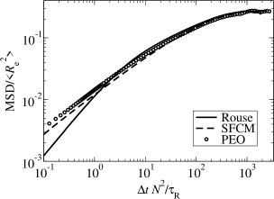
Figure 1: Mean square displacement (MSD) of the monomers in the center-of-mass frame for the Rouse chain, the SFCM and the PEO melt.

A more detailed but related analysis is obtained by directly analyzing the properties of the subdiffusive dynamics. For $\tau_{\mathrm{R}}/N^{2}\leq t\leq\tau_{\mathrm{R}}$, the Rouse theory predicts a subdiffusive motion with a bead mean square displacement proportional to $t^{0.5}$. In contrast to this, a proportionality for the monomer mean square displacement of ${\mathrm{MSD}\left(t\right)}\propto{t^{\alpha}}$ with ${\alpha}\approx{0.6}$ is observed in fig. 1, a value that is generally found in simulations of more realistic polymer models Paul and Smith (2004); Paul (2002); Bulacu and van der Giessen (2005). This indicates that the backdriving forces in a real polymer melt are not only given by the chain connectivity, but also influenced by chain stiffness and intra- and intermolecular excluded volume effects. As an investigation tool for this characteristic dynamics we define the following quantity

$$a=\frac{\langle{\bf r}_{1}\left(t\right){\bf r}_{1}^{\prime}\left(t\right)\rangle}{\langle{\bf r}_{1}^{2}\left(t\right)\rangle}\,,$$ (13)

where ${\bf r}_{1}\left(t\right)$ is the displacement of a given monomer during $t$ and ${\bf r}_{1}^{\prime}\left(t\right)$ subsequent displacement during the next time interval of length $t$. The MSD $\langle{\bf r}_{2}^{2}\left(2t\right)\rangle$ after $2t$ can also be written as the displacement after two successive steps with length $\langle{\bf r}_{1}^{2}\left(t\right)\rangle$ during $t$

$$\langle{\bf r}_{2}^{2}\left(2t\right)\rangle=2\langle{\bf r}_{1}^{2}\left(t\right)\rangle+2\langle{\bf r}_{1}\left(t\right){\bf r}_{1}^{\prime}\left(t\right)\rangle\,,$$ (14)

where the backdriving force is expressed by the second term on the rhs. In cases where the MSD obeys a power law, i.e. $\langle{\bf r}_{1}^{2}\left(t\right)\rangle=\langle{\bf r}_{1}^{\prime 2}\left(t\right)\rangle=ct^{\alpha}$ and $\langle{\bf r}_{2}^{2}\left(2t\right)\rangle=c\left(2t\right)^{\alpha}$, respectively, the exponent $\alpha$ can be related to the backward correlation $a$. By dividing eq. 14 by $\langle{\bf r}_{1}^{2}\left(t\right)\rangle$ and rearranging the expression one obtains

$$\alpha=1+\log_{2}\left(1+a\right)\,.$$ (15)

Figure 2 studies the backward correlation $a$ (left axis) and the exponent $\alpha$ (right axis) for the simulated Rouse chain, the SFCM and the PEO melt (the dotted line corresponds to a freely diffusing particle). The dynamics of the Rouse model for very short times is essentially uncorrelated to its past, as the beads do not experience the connectivity constraint yet (fig. 2). For larger times one observes a long crossover to sublinear diffusion ending in a minimum with $\alpha=0.5$. Note that the time window for this characteristic motion is rather short due to the short chain length ($N=16$). In contrast to this, the local bending potential of the SFCM will immediately push back a monomer bending too far out of the chain curvature. Thus, for the SFCM, the motion of a monomer is very early dominated by backjumps. For larger time scales, $a$ remains nearly constant for the SFCM over several orders of magnitude with slight deviations from ideal behavior (${\alpha}\approx{0.6-0.65}$).

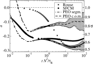
Figure 2: Correlation of two successive displacement vectors (left axis) and exponent of the MSD calculated by eqn 15 (right axis). The dotted line indicates the respective values of a freely diffusing particle.

To a first approximation the PEO dynamics closely resembles the SFCM dynamics in agreement with our observations from the MSD. First, the dynamics of the PEO monomers crosses over from ballistic to backjump-dominated motion at ${\Delta t_{\mathrm{rel}}}\approx{0.1}$ (i.e. approximately $5\,\mathrm{ps}$, during which the monomers move on average $0.75$ times the chemical bond length $b_{0}$). The minimum at ${\Delta t_{\mathrm{rel}}}\approx{0.1}$ can be identified as the confinement of the PEO monomers in a cage imposed by surrounding monomers in the first coordination sphere. The same effect is also observed for low-molecular fluids Doliwa and Heuer (1998). Second, for $\Delta t_{\mathrm{rel}}\geq 1$ the backward-correlations are again somewhat larger. This can at least partly be related to the subdiffusive center-of-mass motion. For real polymer melts, a slightly subdiffusive behavior (with ${\alpha}\approx{0.8}$) on a time scale shorter than the Rouse time was found in simulations Paul et al. (1991, 1998); Smith et al. (2000); Paul and Smith (2004) and NSE experiments Smith et al. (2000); Zamponi et al. (2008) and is predicted by theoretical analyses Guenza (1999, 2001). This is also confirmed in fig. 2 where we also observe a slightly subdiffusive behavior of the PEO chain’s center-of-mass motion throughout the entire observation time larger than the ballistic regime. The trend of the backward-correlation seems to become weaker with increasing time, however, we cannot make clear predictions within the error bars. The additional backdriving motion acting on the PEO chains has been interpreted within the well known correlation hole picture de Gennes (1979), in which regions of the chain that show correlated motion effectively repel each other for entropic reasons. From theoretical and numerical calculations Wittmer et al. (2007) it was shown that the structure of a polymer chain in the melt can be viewed as a hierarchy of correlation holes throughout several length scales, where the repulsion is decreasing with increasing length scale. Of course, for very long time scales standard diffusive behavior would be observed which is, however, beyond the time scales accessible by our simulations.

V Results of the pq-Method

As motivated above the pq-method is supposed to yield a direct check of the intra-molecular interaction. In particular, the specific terms that cause the deviations of the MSDs average out in the quantity $A\left(\Delta t\right)$.

Figure 3 shows a scatterplot of the $p$- and $q$-values of the PEO melt with $\Delta t=84\,\mathrm{ps}$ as well as the corresponding regression line with slope $A(\Delta t)$ (solid line); see eq. 8.

To superimpose the curves obtained by eq. 8 we normalized $A(\Delta t)$ by the value $k/\zeta=N^{2}/(\pi^{2}\tau_{\mathrm{R}})$ expected for the continuous Rouse chain Doi and Edwards (2003). As mentioned already above, $\Delta t$ was normalized by $\tau_{\mathrm{R}}/N^{2}$, characterizing the local relaxation time scale within the Rouse model. In what follows the normalized time is denoted ${\Delta t_{\mathrm{rel}}}$.

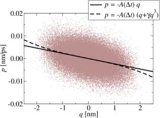
Figure 3: Scatterplot of the corresponding $p$- and $q$-values for the PEO chains with $\Delta n^{\prime}=4$ and $\Delta t=84\,\mathrm{ps}$ as well as the regression line (eq. 7) and an anharmonic third-order fit (eq. 16).

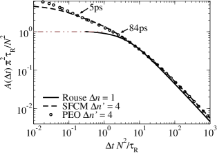
Figure 4: Normalized slope $A\left(\Delta t\right)$ as a function of normalized time for the three different systems analyzed in this work.

The normalized curves for $A_{\mathrm{rel}}(\Delta t_{\mathrm{rel}})$ for a Rouse chain, the SFCM the PEO system are shown in fig. 4. One observes that from about ${\Delta t_{\mathrm{rel}}}\approx{3}$ (i.e. ${\Delta t}\approx{84\,\mathrm{ps}}$) the Rouse and the PEO curve agree very well. At this time, a PEO monomer has moved approximately twice the chemical bond length $b_{0}$, showing that at this point the microscopic influence of the local potentials is averaged out and the coarse-grained Rouse picture becomes applicable. For shorter $\Delta t$ the curve of the Rouse chain converges to the theoretical value of unity. Interestingly, around ${\Delta t_{\mathrm{rel}}}\approx{3}$ the value of $A(\Delta t)$ for the Rouse system has already reached this theoretical short-time limit. One may conclude that at least for PEO the applicability of the Rouse model holds without having to introduce renormalized values for the friction coefficient.

In contrast to the Rouse model, for the SFCM and for PEO $A\left(\Delta t\right)$ further increases with decreasing $\Delta t$. This is a consequence of the chain stiffness which enhances the effect of a local chain curvature. The PEO curve is in perfect agreement with the SFCM from about ${\Delta t_{\mathrm{rel}}}\approx{0.1\mathrm{ps}}$ (${\Delta t}\approx{5\mathrm{ps}}$). Note that this is also the time scale for which the forward-backward coefficient $a$ becomes similar for both systems. This result clearly shows that the dynamical features of a PEO melt are basically captured by the SFCM except for shortest times. The deviations for ${\Delta t}<{5\mathrm{ps}}$ are not due to inertia effects because the velocity autocorrelation function in the MD simulation has already fully decayed around $2\mathrm{ps}$. Thus, the specific properties of the local PEO dynamics is only captured by the SFCM for ${\Delta t}>{5\mathrm{ps}}$.

According to the Rouse model, the restoring force acting on a given bead linearly depends on its elongation (eq. 1), yielding the characteristic harmonic potential. As can already be seen from fig. 3, an anharmonic fit including a third-order term is much more appropriate to describe the data (dashed line). In the following, we wish to examine the assumption of harmonic restoring forces for the SFCM and PEO in more detail. The individual $q$-values were assorted into a histogram, thus yielding the averages $\langle q\rangle$ and $\langle p\rangle$ of the corresponding $p$-values for each bin (fig. 5).

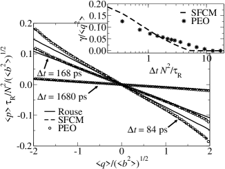
Figure 5: Normalized average $p$ and $q$ values from the histogram of the individual $q$ values for various $\Delta t$. Inset: anharmonicity parameter $\gamma$ defined by eq. 16.

For sufficiently small bead elongations the restoring force indeed is linear. However, when going to larger $q$, this approximation is no longer valid for PEO and the SFCM especially in the limit of short $\Delta t$, and anharmonicities become noticeable. For the SFCM and for PEO, the anharmonicities are similarly pronounced, thus again highlighting that the SFCM effectively incorporates many non-idealities of the PEO melt despite its simplicity. The inset in fig. 5 shows the normalized anharmonicity parameter $\gamma$ defined by

$${\bf p}\left(\Delta t\right)=-A\left(\Delta t\right)\left({\bf q}+\gamma{\bf q}^{3}\right)$$ (16)

when additionally considering third-order terms. The anharmonicity expressed by $\gamma$ for both systems decays on the same timescale. At ${\Delta t_{\mathrm{rel}}}\approx{3}$, where the average bead mobilities of PEO and the Rouse chain become comparable (fig. 4), $\gamma$ has nearly decayed to zero. Although the SFCM and the PEO chains show an anharmonic behavior at large elongations $q$, the linear dependence of the restoring force as assumed in the Rouse model is valid to a good approximation. Deviations become significant only on time scales below the Rouse regime. One might argue that the nonlinear dependence of $p$ on $q$ leads to higher values of $A\left(\Delta t\right)$ for short $\Delta t$, while for larger $\Delta t$ and vanishing anharmonicities the curves of PEO and the SFCM converge to the Rouse curve (fig. 4). However, we find that the data points for large $q$-values in figs. 3 and 5, where higher-order terms become important, have a statistical weight that is negligible compared to the $q$ values near zero. Consistently, the overall value for $A\left(\Delta t\right)$ does not change significantly when the large $q$-values are excluded from the calculation.

VI Conclusions and Outlook

In this article, we presented the pq-method to extract the effective bead mobility from simulation data of polymeric systems. From a conceptual point of the view the main advantage is the direct accessibility of the intra-chain interaction effects. In contrast to this, the analysis of, e.g., the MSD, immediately also involves possibly complex inter-chain contributions. In this way it became possible to show that the SFCM is a perfect model for PEO already for relatively short time scales. Furthermore we could show that the dynamics of the discrete Rouse model is still characterized by the bare friction coefficient at the shortest relevant time scale of $84\mathrm{ps}$.

However, also from a practical perspective the pq-method has a broad range of applications. For example it is possible to determine the friction coefficient of the $n$-th monomer. This may be of importance if the friction coefficients are heterogeneously distributed. Examples are polymer mixtures (e.g. PEO/PMMA) where the local structure of the slow component may determine the local mobility of the fast component. More generally, a detailed characterization of local dynamic properties becomes accessible. In contrast, observables such as the MSD already contain in an uncontrolled way dynamic contributions from adjacent monomers or even complete Rouse modes, thus invalidating a strictly local analysis. Furthermore, the pq-method can be directly applied to the analysis of topologically more complex systems (e.g. branched polymers) where the local friction coefficient may be directly calculated, e.g., in dependence of the distance to the main chain.