From Phase Space Representation to Amplitude Equations in a Pattern Forming Experiment

Abstract

We describe and demonstrate a method to reconstruct an amplitude equation from the nonlinear relaxation dynamics in the succession of the Rosensweig instability. A flat layer of a ferrofluid is cooled such that the liquid has a relatively high viscosity. Consequently, the dynamics of the formation of the Rosensweig pattern becomes very slow. By sudden switching of the magnetic induction, the system is pushed to an arbitrary point in the phase space spanned by the pattern amplitude and the magnetic induction. Afterwards, it is allowed to relax to its equilibrium point. From the dynamics of this relaxation, we reconstruct the underlying fully nonlinear equation of motion of the pattern amplitude. The measured nonlinear dynamics serves to select the best weakly nonlinear expansion which describes this hysteretic transition.

1 Introduction

When aristotle350 described the motion of falling bodies, he incorrectly claimed that the velocity is constant and proportional to the mass of the body, because he did not know the concept of inertia. He has been later proven wrong by galileo1638 and newton1687, who linked acceleration with forces. Aristotles’ idea of motion, however, is a valid approximation in many cases, when a viscous fluid is involved and either the typical dimension $d$ and the velocity $v$ are small, or the kinematic viscosity $\nu$ is high. In this limiting case of small Reynolds numbers $\mathit{Re}={vd}/{\nu}\ll 1$, the viscous forces outweigh inertia, and body and fluid motion is determined entirely by drag forces. Therefore, from a measurement of the velocity field one immediately obtains the acting forces.

A similar dynamics is expected in the neighbourhood of a hydrodynamic instability, namely an amplitude equation of the form $\partial A/\partial t=f(A)$. The coefficients of these functions $f$ can be determined experimentally. As an early example, wesfreid1978 accomplished this in a Rayleigh-Bénard convection experiment by observing the relaxation of the pattern amplitude following a jump in the control parameter. In this way, the coefficients of the amplitude equation of a pitchfork forward bifurcation to stripe-like patterns had been obtained. Here we present such a measurement technique for a transcritical bifurcation to hexagons, which is characteristic for systems with broken up–down symmetry, i.e. a different universality class. As a specific example, we study the hexagonal arrangement of spikes forming in a layer of magnetic fluid.

Magnetic fluids, also known as ferrofluids, are colloidal suspensions of magnetic nanoparticles [rosensweig1985]. When a vertically oriented magnetic field is applied to a horizontal layer of ferrofluid, then a regular pattern of liquid spikes can appear above a certain threshold value of the magnetic induction $B_{c}$. This normal field instability was first reported by cowley1967 and is thus also known as the Rosensweig instability. For an infinitely deep container, these authors provide also a linear stability analysis to find the critical threshold $B_{c}$ of the magnetic induction and the critical wave number $k_{c}$. Their analysis works by computing the dynamics of a regular pattern in the vicinity of the threshold induction and for very small amplitudes. This approach has later been extended to calculate the viscosity dependent growth rate by salin1993, and a finite depth of the container was taken into account by weilepp1996. For the case of a viscous magnetic fluid and an arbitrary layer thickness, lange2000 derived the growth rate and the wave number of maximal growth. The latter is experimentally determined and compared with the theoretical predictions in the same article, and later on compared with the wave number of the nonlinear state [lange2001]. lange2001b calculates the growth rate for ferrofluids of different viscosity and eventually extends his analysis to the case of a nonlinear magnetization curve [knieling2007pre].

The nonlinear aspects of the dynamics have posed additional difficulties to the theoretical analysis [lange2002adjoint]. Only recently, bohlius2007adjoint bohlius2007adjoint,bohlius2008amplitude successfully tackled the issue of systematically deriving nonlinear amplitude equations. For the amplitude $A$ of hexagonal patterns these authors obtained

$$\tau_{0}\frac{\partial A}{\partial t}=\varepsilon A+\gamma_{1}A^{2}-gA^{3}.$$ (1)

Here, $\tau_{0}$ denotes a time scale, $\varepsilon=(B^{2}-B_{c}^{2})/B_{c}^{2}$ measures the distance from the bifurcation point, and $\gamma_{1}$ and $g$ are expansion coefficients. The static solution of this amplitude equation coincides in structure with the result presented by gailitis1977 and by kuznetsov1976b, which was derived for magnetic susceptibilities $\chi\ll 1$ using an energy minimization approach. Using a similar approach, friedrichs2001 present a solution which is applicable up to $\chi\leq 0.4$. This solution is slightly different and corresponds to the amplitude equation with

$$\tau_{0}\frac{\partial A}{\partial t}=\varepsilon A+\gamma_{1}\left(1+\varepsilon\right)A^{2}-gA^{3}.$$ (2)

The difference to the cubic equation (1) is the additional factor $\left(1+\varepsilon\right)$ in the quadratic term. The physical reasoning behind this higher order correction is a scaling of the quadratic coefficient with $B^{2}$, which is proportional to $1+\varepsilon=B^{2}/B_{c}^{2}$. In the limit of $\varepsilon\to 0$, both equations coincide. Now the question arises, which of these solutions compares best to the experiment.

So far, the static solution of equation (2) was successfully fitted to the measured pattern amplitude for a ferrofluid with high susceptibility [richter2005] and moderate susceptibility [gollwitzer2007]. However, the amplitude equation (1) provides much more information, specifically the nonlinear dynamics of the pattern formation. This has not yet been exploited. knieling2007pre observed the nonlinear dynamics in a previous experiment and in related numerical simulations, but a quantitative comparison to an analytical model is performed only in the linear regime of the pattern growth.

The key idea in this paper is now to use a fluid with a very high viscosity to study the pattern formation of the Rosensweig instability. Consequently, the Reynolds number is very small $\mathit{Re}\approx 10^{-3}$, and the relaxation is monotonic and slow. The heavily overdamped system makes it easy to study the nonlinear dynamics quantitatively: due to the strong damping, the pattern amplitude follows a first order equation of motion

$$\frac{\partial A}{\partial t}=f(\varepsilon,A)$$ (3)

even in the nonlinear regime. Here $f$ is an analytic function, which does not directly depend on the time $t$. From the experimental data, $f$ can be reconstructed and directly compared to the theoretical amplitude equations.

In the next section, we describe the experimental setup and the magnetic fluid we use. Subsequently, the measurement protocol and the data analysis are described. Then the experimental data are compared to theoretical models, and finally the results are discussed.

2 Experimental setup

Figure 1: Setup of the apparatus for dynamic measurements of the Rosensweig instability. Scheme of the assembled setup (a), and exploded view of the container with the coils (b).

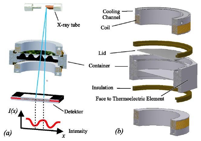
The experimental setup for the measurements of the surface deflections consists of an X-ray apparatus described in detail by richter2001. An X-ray point source emits radiation vertically from above through the container with the ferrofluid, which is placed midway between a Helmholtz pair of coils. Underneath the container, an X-ray camera records the radiation passing through the layer of ferrofluid. The intensity at each pixel of the detector is directly related to the height of the fluid above that pixel. Therefore, the full surface topography can be reconstructed after calibration [gollwitzer2007].

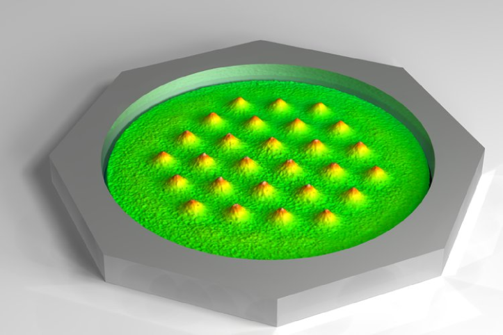
The container, which holds the ferrofluid sample, is depicted in figure 1(b). It is a regular octagon machined from aluminium with a side length of $77\,\mathrm{mm}$ and two concentric inner bores with a diameter of $140\,\mathrm{mm}$. These circular holes are carved from above and below, leaving only a thin base in the middle of the vessel with a thickness of $2\,\mathrm{mm}$. On top of the octagon, a circular lid is placed, which closes the hole from above (see figure 1b). Each side of the octagon is equipped with a thermoelectric element QC-127-1.4-8.5MS from Quick-Ohm. These are powered by a $1.2\,\mathrm{kW}$ Kepco KLP-20-120 power supply. The hot side of the thermoelectric elements is connected to water cooled heat exchangers. The temperature is measured at the bottom of the aluminium container with a Pt100 resistor. A closed loop control, realized using a computer and programmable interface devices, holds the temperature $\theta$ of the vessel constant with an accuracy of $10\,\mathrm{mK}$.

The container is surrounded by a Helmholtz pair of coils, thermally isolated from the vessel with a ring made from a flame resistant composite material (FR-2). The size of the coils is adapted to the size of the vessel in order to introduce a magnetic ramp. With these coils, the magnetic field strength falls off towards the border of the vessel, where it reaches $80\,\%$ of its value in the centre. For details of the magnetic ramp see knieling2010. Filling the container with ferrofluid enhances the magnetic induction in comparison with the empty coils for the same current $I$. Therefore $B(I)$ is measured immediately beneath the bottom of the container, at the central position, and serves as the control parameter in the following.

Table 1: Material properties of the ferrofluid mark APG E32 (Lot G090707A) from Ferrotec Co.

Quantity		Value	Error	Unit
Density	$\rho$	$1168\$	$\pm 1$	$\mathrm{kg\,m^{-3}}$
Surface tension	$\sigma$	$30.9\$	$\pm 5$	$\mathrm{mN\,m^{-1}}$
Viscosity at $10\,$°C	$\eta$	$4.48\$	$\pm 0.1$	$\mathrm{Pa\,s}$
Saturation magnetization	$M_{S}$	$26.6\$	$\pm 0.8$	$\mathrm{kA\,m^{-1}}$
Initial susceptibility at $10\,$°C	$\chi_{0}$	$3.74\$	$\pm 0.005$
Fit of $M(H)$ with the model by ivanov2001:
Exponent of the $\Gamma$-distribution	$\alpha$	$3.8$	$\pm 1$
Typical diameter	$d_{0}$	$1.7$	$\pm 0.2$	$\mathrm{nm}$
Volume fraction	$\phi$	$5.96$	$\pm 0.2$	$\%$
critical induction from $M(H)$	$B_{c}$	10.5	$\pm 0.1$	$\mathrm{mT}$

Figure 2: The dynamic viscosity $\eta$ of the ferrofluid APG E32 versus the temperature $\theta$. The symbols represent measurements, and the solid line is an approximation by equation (4).

Figure 3: Magnetization curve of the ferrofluid APG E32. The symbols show the measured data at $\theta=20\,$°C. The black dashed line marks a fit with the model by ivanov2001. The blue solid line shows an extrapolation to $\theta=10\,$°C according to this model.

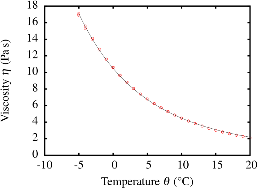
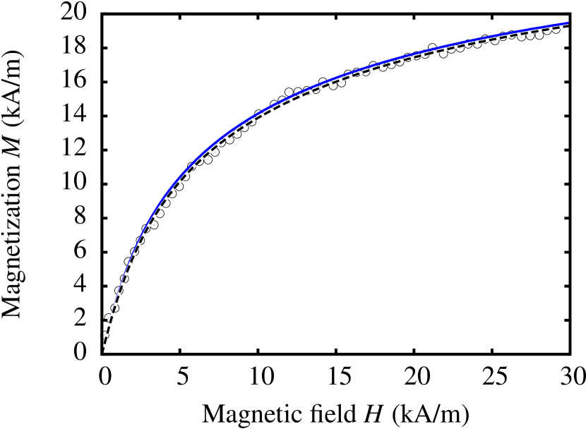
We use the commercial ferrofluid APG E32 from Ferrotec Co, the basic material parameters of which are listed in table 1. The density was measured using a DMA 4100 density meter from Anton-Paar. More problematic is the measurement of the surface tension. We measure the surface tension using a commercial ring tensiometer (LAUDA TE 1) and a pendant drop method (Dataphysics OCA 20). Both methods result in a surface tension of $\sigma=31\pm 0.5\,\mathrm{mN/m}$, but when the liquid is allowed to rest for one day, $\sigma$ drops down to $25\pm 0.5\,\mathrm{mN/m}$. This effect, which is not observed in similar, but less viscous magnetic liquids like APG 512 a, which was used in previous work [gollwitzer2009nfi], gives a hint that our liquid is chemically less stable in the sense that the surfactants change the surface tension on a longer time scale, when the surface is changed. Since the pattern formation experiments do change the surface during the measurements, the uncertainty of the surface tension is about $5\,\mathrm{mN/m}$, as given in table 1.

The viscosity $\eta$ deserves a special attention for the experiments in this paper, as it influences the time scale of the pattern formation. It has been measured in a temperature range of $-5\,\textrm{\textdegree C}\leq\theta\leq 20\,\textrm{\textdegree C}$ using a commercial rheometer (MCR 301, Anton Paar) in cone and plate geometry (figure 3). At room temperature, the ferrofluid we use has a viscosity $\eta=2\,\mathrm{Pa\,s}$, i.e. 2000 times the viscosity of water. This value can be increased by a factor of $9$ when the liquid is cooled to $-5\,$°C. The data from figure 3 can very well be fitted with the Vogel-Fulcher law [rault2000vogelfulcher]

$$\eta=\eta_{0}\exp\left(\frac{\psi}{\theta-\theta_{0}}\right),$$ (4)

with $\eta_{0}=0.48\,\mathrm{mPa\,s},\psi=1074\,\mathrm{K},$ and $\theta_{0}=-107.5\,$°C, as marked by the solid line in figure 3. This means, that the viscosity can easily be adjusted in a wide range by controlling the temperature. For the present measurements, we chose a temperature of $\theta=10\,$°C, where the viscosity amounts to $\eta=4.48\,\mathrm{Pa\,s}$ according to equation (4).

The magnetization curve has been determined using a fluxmetric magnetometer consisting of a Helmholtz pair of sensing coils with $6800$ windings and a commercial integrator (Lakeshore Fluxmeter 480). The sample is held in a spherical cavity with a diameter of $12.4\,\mathrm{mm}$ in order to provide a homogeneous magnetic field inside the sample with a demagnetization factor of $\frac{1}{3}$. The magnetization curve has been measured at a temperature of $\theta=20\,$°C (see figure 3). For a comparison with the pattern formation experiments, this curve must be extrapolated to $\theta=10\,$°C, which is done using the model by ivanov2001. Following rosensweig1985, § 7.1, from this curve and the material parameters a critical induction of $10.5\,\mathrm{mT}$ is estimated (c.f. table 1).

3 Measurement protocol

Figure 4: The multistep measurement protocol for the relaxation measurements. Dotted arrows indicate jumps of the magnetic inductions. Blue arrows denote the path of the system during the relaxation phases. A movie which shows the sequence 1–2a is available from http://ep5.uni-bayreuth.de/ff/movies/Frozensweig2a.html

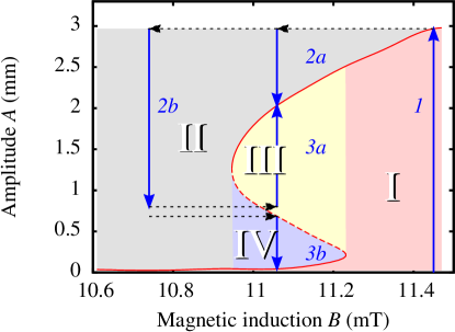
Figure 4 displays the measurement protocol on the basis of the bifurcation diagram. The static pattern amplitude of the Rosensweig instability in our fluid is indicated by the red line. When the system is set onto an arbitrary initial point $(B_{\textrm{\scriptsize ini}},A_{\textrm{\scriptsize ini}})$ in this diagram, and the magnetic induction $B$ is kept constant, the amplitude $A$ monotonically increases or decreases, until the system reaches the stable equilibrium (solid red line). The direction of the change of $A$ depends on the region, where $(B_{\textrm{\scriptsize ini}},A_{\textrm{\scriptsize ini}})$ is situated – in the regions I and III in figure 4, $A$ increases, and in regions II and IV, the amplitude decreases with time.

In order to push the system to an arbitrary initial location $(B_{\textrm{\scriptsize ini}},A_{\textrm{\scriptsize ini}})$, a multistep measurement protocol is employed. The first step (path 1) is always a relaxation of the pattern in region I at the overcritical induction $B_{\textrm{\scriptsize high}}=11.45\,\mathrm{mT}$ for $1\,\mathrm{min}$, to reach the final amplitude of $A_{\textrm{\scriptsize high}}=2.98\,\mathrm{mm}$ at that point. The corresponding pattern is shown in figure 5(a). To get to an arbitrary point in the region II in diagram 4, a second step is needed. When the system is settled at $(B_{\textrm{\scriptsize high}},A_{\textrm{\scriptsize high}})$, the magnetic induction is quickly changed to the desired value $B_{\textrm{\scriptsize ini}}$, and the resulting dynamics is observed (path 2a), until the final amplitude is reached. To get into the inner regions III or IV, three steps are needed in total – coming from $(B_{\textrm{\scriptsize high}},A_{\textrm{\scriptsize high}})$, the second step (path 2b) is a decay of the pattern amplitude at the subcritical induction $B_{\textrm{\scriptsize low}}=10.74\,\mathrm{mT}$, until the intended initial amplitude $A_{\textrm{\scriptsize ini}}$ is reached. The induction is then quickly raised to the desired $B_{\textrm{\scriptsize ini}}$. The system then follows the path 3a or 3b in region III or IV, respectively.

When the desired initial amplitude $A_{\textrm{\scriptsize ini}}$ is zero, for example when the growth of the pattern in region I shall be observed, we also apply the three step protocol with the detour by paths 1 and 2b. At this point, the pattern decays until the amplitude is very small ($A_{\textrm{\scriptsize ini}}=0.05\,\mathrm{mm}$). After that, the induction is raised to $B=B_{\textrm{\scriptsize ini}}$. We use this procedure instead of directly switching the magnetic induction from zero to $B=B_{\textrm{\scriptsize ini}}$ in order to establish the exact same pattern in all regions. Coming from a perfectly flat surface, the pattern would have additional degrees of freedom manifesting themselves in point defects or different orientations of the wave vectors. When we take the detour by the paths 1 and 2b, we seed the wave vectors of the pattern at $(B_{\textrm{\scriptsize high}},A_{\textrm{\scriptsize high}})$, and the final pattern developed is likely to be the same.

We explored all regions in figure 4 in several rounds. In the first round, we examined region I. We used the three step procedure to observe the growth of the pattern from a very small amplitude up to the stable solution for $21$ different inductions in the range $11.19\,\mathrm{mT}\leq B\leq 11.46\,\mathrm{mT}$. In the second round we explored region II. Starting from $A_{\textrm{\scriptsize ini}}=A_{\textrm{\scriptsize high}}$ and $65$ different inductions in the range $10.61\,\mathrm{mT}\leq B\leq 11.46\,\mathrm{mT}$, the decay of the pattern was observed until it reaches the stable solution or zero. The third to sixth rounds covered the regions III and IV. Starting from four different amplitudes, we observed the evolution of the pattern in the range of $10.89\,\mathrm{mT}\leq B\leq 11.27\,\mathrm{mT}$. At each round, we recorded the complete evolution of the surface topography of the ferrofluid during the last step with the fastest possible frame rate ($7.5\,\mathrm{Hz}$) of the X-ray device, in total taking about $170\,000$ frames.

4 Data analysis

4.1 Reconstruction of the pattern amplitude

(a)

(b)

Figure 5: The final pattern at $B=11.45\,\mathrm{mT}$. Chart (a) displays a reconstruction of the surface in real space. The outer dimension of the container is not to scale. The colour code gives the height of the liquid surface above ground in mm. The pattern amplitude is determined from the corresponding power spectrum shown in (b) by the total power in the encircled mode.

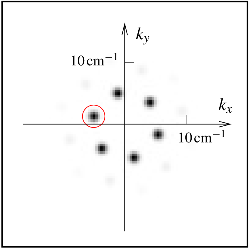
After processing the image data, we finally arrive at the surface topography for every frame. Figure 5(a) shows a reconstruction of the surface at $B=B_{\textrm{\scriptsize high}}$. A description of the technical details of this process can be found in the paper by gollwitzer2007. The amplitude of the pattern, $A$, is then determined in Fourier space (figure 5b). We use a circularly symmetric Hamming window with the weight function

$$w(x,y)=\cases{\left(0.54+0.46\cos\left(\frac{\pi\sqrt{x^{2}+y^{2}}}{r_{w}}\right)\right)^{2}&$x^{2}+y^{2}\leq r_{w}^{2}$\\ 0&else\\ }$$ (5)

for apodization [gollwitzer2006b] with a radius $r_{w}=46\,\mathrm{mm}$. The total power in one of the modes (marked with a red circle in figure 5b) is used to compute the amplitude of the pattern

$$A=N\cdot\sqrt{\sum_{j}\left|c_{j}\right|^{2}},$$ (6)

where $c_{j}$ are the Fourier coefficients inside the circle. In order to get a meaningful estimate, the normalization factor $N$ is chosen such that $A$ is the height difference between maxima and minima, when the input is a perfectly sinusoidal hexagonal pattern.

(a)

(b)

Figure 6: The evolution of the pattern amplitude at an induction $B=11.06\,\mathrm{mT}$, starting from different amplitudes (a). The labels of the datasets correspond to the paths in figure 4. The path 3c ends in a localized state with only one spike (X-ray image shown in b), and has been removed from the data. A movie showing the temporal evolution of the pattern to the final state in (b) is available from http://ep5.uni-bayreuth.de/ff/movies/Frozensweig3c.html

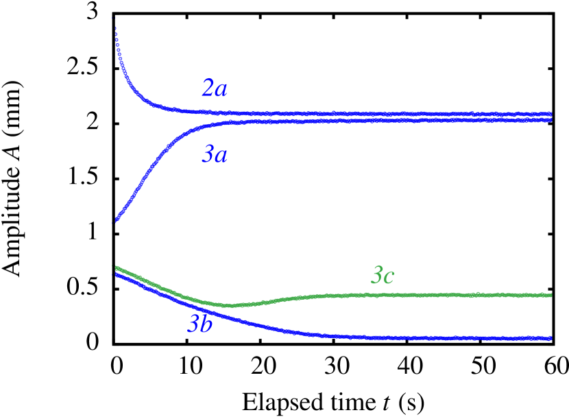
Figure 6(a) displays the resulting amplitude versus time for the paths labelled 2a, 3a and 3b in figure 4. As expected from the bifurcation diagram, the amplitudes for paths 2a and 3b decrease monotonically, and the stable solution is approached in an asymptotic fashion. Similarly, 3a increases monotonically and asymptotically converges to the patterned state. There is, however, a small glitch. The bifurcation diagram 4 provides only a single solution for the patterned state, but the asymptotic amplitudes of the paths 2a and 3a differ by $2.6\,\%$. The reason is that the final pattern is different, in spite of the aforementioned efforts – path 2a ends in a pattern with $20$ spikes, whereas the final pattern of path 3a contains only $11$ spikes. These additional spikes are situated near the border of the window function and therefore contribute only little to the overall amplitude. A further path, 3c, which starts very close from the initial amplitude of the path 3b, ends in a finite intermediate amplitude. Path 3c finally ends in a localized solution with only one single spike as depicted in figure 6(b).

We are currently unable to control these additional degrees of freedom for the system. In the following, the datasets with a reduced number of spikes have not been treated in a special way. Only when the final pattern does not fill the full width at half maximum of the window function, that is for less than $10$ spikes, the estimated amplitude would be more than $9\,\%$ too small for the given window function. These datasets have been sorted out.

Out of $205$ datasets, $32$ have been rejected, the final pattern of which consists of only a small number of spikes. Every pattern from a single spike up to a cluster of $9$ has been found, whereas the fully developed pattern contains up to $27$ spikes. These patterns emerged in the bistable regime of the fully developed pattern and have been previously observed by richter2005. In their experiment, the localized spikes have been initiated by a local disturbance of the magnetic induction. In the present experiment, these patterns emerge spontaneously from a starting point $(B_{\textrm{\scriptsize ini}},A_{\textrm{\scriptsize ini}})$ near the unstable solution branch. In this study, however, we focus only on the fully developed patterns.

4.2 Recovery of the amplitude equation

Figure 7: Reconstruction of the amplitude equation at an induction $B=11.05\,\mathrm{mT}$. The symbols are central differences from equation (7). The red line serves as a guide to the eye. The blue arrows indicate the range of the corresponding data sets presented in Fig. 6 (a).

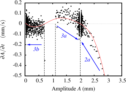
In the following, we will describe a method to extract the amplitude equation from the experimental data. So far, we have measured the evolution of the amplitude $A(t)$ for different values of the induction $B$ and a set of initial amplitudes $A_{\textrm{\scriptsize ini}}$. Suppose, that the system can indeed be described by an amplitude equation of the form (3). Then $A(t)$ is the solution of this equation for different initial conditions $(B_{\textrm{\scriptsize ini}},A_{\textrm{\scriptsize ini}})$, and we want to get the function $f$ on the right hand side of (3). Because this function should not depend on time, the time derivative $\dot{A}=\partial A/\partial t$ of our measured $A(t)$ directly gives the value of this function at the corresponding amplitude. We therefore plot $\dot{A}$ as a function of $A$ in figure 7 for one selected induction in the bistable region. The time derivative has been estimated from the measured data by central differences [abramowitz1970, §25.1.2]

$$\left.\frac{\partial A}{\partial t}\right|_{n+\frac{1}{2}} \approx \frac{A_{n+1}-A_{n}}{\Delta t}$$

$$\left.A\right|_{n+\frac{1}{2}} \approx \frac{A_{n+1}+A_{n}}{2},$$ (7)

where $\Delta t=0.134\,\mathrm{ms}$ is the time between consecutive frames, and $A_{i}$ denotes the pattern amplitude of the $i$^th frame. The plot in figure 7 comprises three different data sets. The sets 2a and 3a stem from a relaxation to a pattern amplitude of about $2\,\mathrm{mm}$; set 3b describes the decay to a flat surface layer. Because the time derivative of the experimental data suffers heavily from noise, we also plot a smooth approximation explained later in § 5 as a guide to the eye (red line in figure 7). In the bistable regime, the amplitude equation has three roots, corresponding to one unstable and two stable solutions. In figure 7, these stable and unstable solutions are characterized by zero-crossings with a negative or positive slope, respectively.

5 Experimental results

Figure 8: The measured amplitude dynamics for the whole phase space. The colour indicates the velocity $\partial A/\partial t$ in mm/s. Red (blue) means rising (falling) amplitude, respectively. Green indicates the zero (root of the amplitude equation).

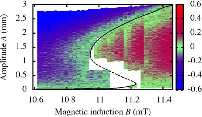
Figure 8 displays the dynamics of the amplitude determined from equation (7) in the full range of $A$ and $B$. The colour indicates sign and strength of the "force" $f(B,A)$ and confirms the bifurcation diagram suggested in figure 4. However, the data points are not only affected by noise, they are also irregularly distributed. The density is high at the stable solution branch, and on the contrary there are voids in the diagram, where no data is available at all. These voids belong to data sets which have been sorted out, because they converge to a localized solution (cf. § 4.2).

In order to further interpret the data, a smooth approximation is helpful. The next section shows a way to construct such an approximation. Thereafter it is compared with analytical model equations (§ 5.2)

5.1 Approximation with radial basis functions

Figure 9: The multiquadric RBF approximation of $\partial A/\partial t(A,B)$. The colour indicates this velocity in mm/s. The red dots correspond to the measured data. The blue crosses show the position of the centres of the radial basis functions. The black solid (dashed) line represents the stable (unstable) zero of the approximant.

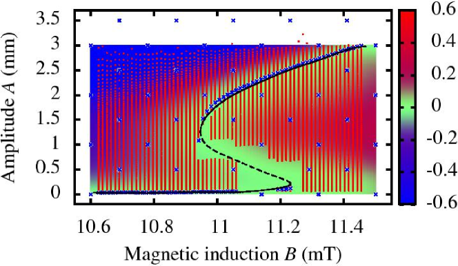
We use a multiquadric radial basis function (RBF) network to compute a smooth sensible approximation to the amplitude equation [powell1990rbftheory]. A RBF network is a linear combination of shifted basis functions

$$s(\boldsymbol{x})=\sum_{j}\lambda_{j}\phi(\left\|\boldsymbol{x}-\boldsymbol{c}_{j}\right\|)+p(\boldsymbol{x}),$$ (8)

with the weights $\lambda_{j}$, a basis function $\phi$, the arbitrarily chosen centres $\boldsymbol{c}_{j}$ and the low order multivariate polynomial $p(\boldsymbol{x})$. We choose the multiquadric basis function

$$\phi(x)=\sqrt{1+x^{2}}$$ (9)

and a linear polynomial $p(\boldsymbol{x})$. The vector $\boldsymbol{x}$ is a scaled combination of the coordinates of the phase space

$$\boldsymbol{x} = \left(B/\delta_{B},A/\delta_{A}\right)$$ (10)

$$\delta_{B} = 0.2\,\mathrm{mT}$$

$$\delta_{A} = 1\,\mathrm{mm}.$$

The scale variables $\delta_{A,B}$ are chosen according to the empirical rule, that they should be approximately equal to the distance between centres in the corresponding direction.

RBF networks with the basis function (9) are infinitely differentiable and thus well-suited to the approximation of smooth functions. This kind of approximation has been proven useful in many applications. For an overview, see the review by hardy1990rbf.

Figure 9 displays the result from fitting the measured data from figure 8 with equation (8). The centres $\boldsymbol{c}_{j}$ can be chosen almost arbitrarily; we have selected $50$ centres equally distributed in the measured region and additionally placed $68$ centres near the stable solution branch. The location of these $118$ centres is marked in figure 9 by the blue crosses.

Only the weights $\lambda_{j}$ in equation (8) are adjusted, while the position of the centres $\boldsymbol{c}_{j}$ are held constant. The problem of adjusting equation (8) to our data is therefore reduced to a general linear least squares fitting problem with $118$ free parameters. In order to avoid the problem of overfitting, we do not fit the data directly with equation (8), but instead apply Tikhonov regularization [neumaier1998regularization]

$$\sum_{j}\left|s(\boldsymbol{x}_{j})-f(\boldsymbol{x}_{j})\right|^{2}+\xi\sum_{k}\lambda_{k}^{2}\ =\textrm{min!},$$ (11)

where $f(\boldsymbol{x}_{j})$ are the measured data and $\xi$ is the regularization parameter. This parameter controls the complexity of the model. A value near zero results in a standard least squares fit of the model to the data, while a larger value makes the resulting model more smooth. To find the optimal value for the regularization parameter, we apply standard 2-fold cross validation [picard1984gcv], which yields an optimal regularization parameter of $\xi=0.4$.

The zero from this fit gives an estimate for the stable and unstable solution of the amplitude equation and is indicated by the solid and dashed black line in figure 9, respectively. For comparison, the original data are also shown with the red dots. The RBF reconstruction of the solution gives a very plausible result, which captures the essential features of the raw data, namely the imperfection, and provides an estimate for the unstable solution, which can only be approached to a certain limit by this method (see the voids in diagram 8). This result of the RBF reconstruction has also been used to display the equilibrium in the figures 4 and 8 above.

Such an approximation of the measured data by a RBF network has proven useful to get an unbiased estimate of the equilibrium and to fill in missing data. However, such a non-parametric regression technique cannot provide physically meaningful parameters [green1994nonparametric]. In the next section, we compare the experimental data with nonlinear model equations for the bifurcation.

5.2 Comparison to nonlinear model equations

A model equation for the imperfect, hysteretic bifurcation diagram like in figure 4 is given by

$$\tau_{0}\frac{\partial A}{\partial t}=\varepsilon A+\gamma_{1}\left(1+\gamma_{2}\varepsilon\right)A^{2}-gA^{3}+b,$$ (12)

where $\tau_{0}$ denotes a time scale and $\varepsilon=(B^{2}-B_{c}^{2})/B_{c}^{2}$ measures the distance from the bifurcation point [reimann2005]. For the diagram depicted in figure 4, $\gamma_{1}$ must be positive, and the width of the hysteresis increases with the magnitude of $\gamma_{1}$. In order to get stable patterns for $\varepsilon>0$, $g$ must be positive, and the final amplitude decreases with the magnitude of $g$. The constant term $b$ represents the imperfection of the system. For $b>0$, the transcritical bifurcation at $\varepsilon=0,A=0$ dissolves into two saddle-node bifurcations, the distance of which is controlled by the magnitude of $b$.

In the perfect case ($b=0$) and for $\gamma_{2}=0$ equation (12) simplifies to equation (1). For $\gamma_{2}=1$ equation (12) comprises the amplitude equation (2), where the quadratic term is augmented by the factor $\left(1+\varepsilon\right)$. From a formal point of view, one might ask, whether this additional factor could also incorporate another adjustable parameter, the blend parameter $\gamma_{2}$, resulting in the more general equation (12). Therefore, a comparison of the experimental data with this equation provides some hint, whether it is empirically advantageous to incorporate the $\varepsilon$-dependence in the quadratic coefficient.

The coefficients in the equations (1) and (2) are in principle given by bohlius2008amplitude and friedrichs2001, respectively, as functions of the material parameters. However, these analyses are carried out for a linear magnetization curve $M(H)=\chi H$ and, in the latter case, small values of $\chi$ only, and therefore cannot be directly applied to our fluid. By treating $\tau_{0},B_{c},\gamma_{1},\gamma_{2},g,$ and $b$ as adjustable parameters, these equations can nevertheless be fitted to the measured data. The coefficients are listed in table 2.

Figure 10: Comparison of different models for the amplitude equation. (a) cubic equation (1), (b) augmented equation (2), and (c) blended equation (12) with $\gamma_{2}=0.755$. The white line is the neutral curve obtained from the RBF approximation, while the black line and the colour code comes from the corresponding model.

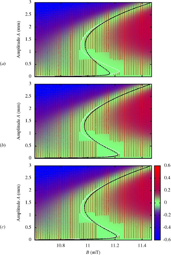
Figure 10 displays the result of fitting the model equations to the experimental data together with the neutral curve of the RBF approximation (white line) for reference. At a first glance, all models give reasonable approximations to the experimental data and the differences are minor. One such difference becomes apparent when looking at the equilibrium line (black solid line). The experimental data (red dots) evidently contain the final static amplitude in almost all cases, so the equilibrium should pass through, or very nearby the endpoints of the experimental data lines. This condition does not hold for the plain cubic equation in figure 10(a). The width of the bistable regime $\Delta B_{\textrm{\scriptsize hyst}}$ suggested by the experimental data amounts to $0.29\,\mathrm{mT}$, but the cubic equation provides only $0.18\,\mathrm{mT}$ (c.f. table 2). The equation (2), which is augmented with $\left(1+\varepsilon\right)$, gives a much better approximation of the equilibrium line (figure 10b). Here, the width of the hysteresis amounts to $0.25\,\mathrm{mT}$, which is better but still smaller than the true value. Finally equation (12), which is a blend of the two former models, scores in between them in this test with $\Delta B_{\textrm{\scriptsize hyst}}=0.24\,\mathrm{mT}$ (figure 10c). The comparison of $\Delta B_{\textrm{\scriptsize hyst}}$ takes only the two saddle-node points into account. To compare the whole equilibrium line, we provide an integral measure, namely the deviation in $B$ on the static solution

$$\aleph=\frac{1}{A_{\textrm{\scriptsize max}}\cdot\bar{B}_{c}^{2}}\int\limits_{0}^{A_{\textrm{\scriptsize max}}}\left(B_{\textrm{\scriptsize RBF}}-B\right)^{2}\mathrm{d}A,$$ (13)

which is integrated over the whole amplitude range covered in the experiment. Here, $B_{\textrm{\scriptsize RBF}}$ serves as a smooth approximation to the experimental data, and $\bar{B}_{c}=11.36\,\mathrm{mT}$ is the mean value of the critical inductions of the three model equations.

For a list of $\aleph$, see the 7th column of table 2. In this measure, the augmented equation (2) comes closer to the RBF by a factor of $3$. Both inspected measures, $\Delta B_{\textrm{\scriptsize hyst}}$ and $\aleph$ demonstrate that the augmented equation (2) provides a better approximation than the pure cubic equation (1). A description by the blended model (12) yields a best fit blend parameter $\gamma_{2}=0.891$. This tends more to the augmented equation (2) than to the plain cubic equation (1). It is thus safe to conclude, that equation (2) provides a wider range of applicability compared to equation (1), with the same number of adjustable parameters.

Table 2: The different models and their coefficients (columns 1-5). To elucidate their applicability to the experimental data we compare the width $\Delta B_{\textrm{\scriptsize hyst}}$ of the bistable regime, the integral deviation $\aleph$ of the static solutions from the RBF approximation in the investigated range $A\in[0.04\,\mathrm{mm}\dots 2.97\,\mathrm{mm}]$, and the residual sum of squares $\hat{\chi}^{2}$ of all time dependent data (columns 6-8). For the amplitude equations, also the critical threshold $B_{c}$ is given in the last column.

Model	$\tau_{0}$	$\gamma_{1}$	$\gamma_{2}$	$g$	$b$	$\Delta B_{\textrm{\scriptsize hyst}}$	$\aleph$	$\hat{\chi}^{2}$	$B_{c}$
	(s)	$(\mathrm{1/mm})$		$(\mathrm{1/mm^{2}})$	$(\mathrm{mm})$	($\mathrm{mT})$	$10^{-6}$	$(\mathrm{mm/s})^{2}$	$(\mathrm{mT})$
Eq. (1)	0.4897	0.0773	$0$	0.0297	0.0013	0.1809	7.58	327.638	11.27
Eq. (2)	0.5933	0.1171	$1$	0.0407	0.0024	0.2468	2.56	326.834	11.40
Eq. (12)	0.5770	0.1111	$0.891$	0.0391	0.0023	0.2372	2.85	326.816	11.39
RBF	N/A	N/A	N/A	N/A	N/A	0.2834	N/A	278.12	N/A

(a)

(b)

Figure 11: Comparison of the amplitude equations for a constant induction $B=10.80\,\mathrm{mT}$ (a) and $B=11.35\,\mathrm{mT}$ (b). The symbols display the original measured data, the dashed line is the RBF approximation, and the solid lines represent the parametric model equations (1, red), (2, blue) and (12, green).

Figure 12: Comparison of the time evolution of the amplitude for the paths 2a and 2b with the integrated model equations. The black dots display the original measured data, the lines represent the solution of equation (3) for different right hand sides, namely RBF (red dashed line) and the amplitude equations (1, red), (2, blue) and (12, green).

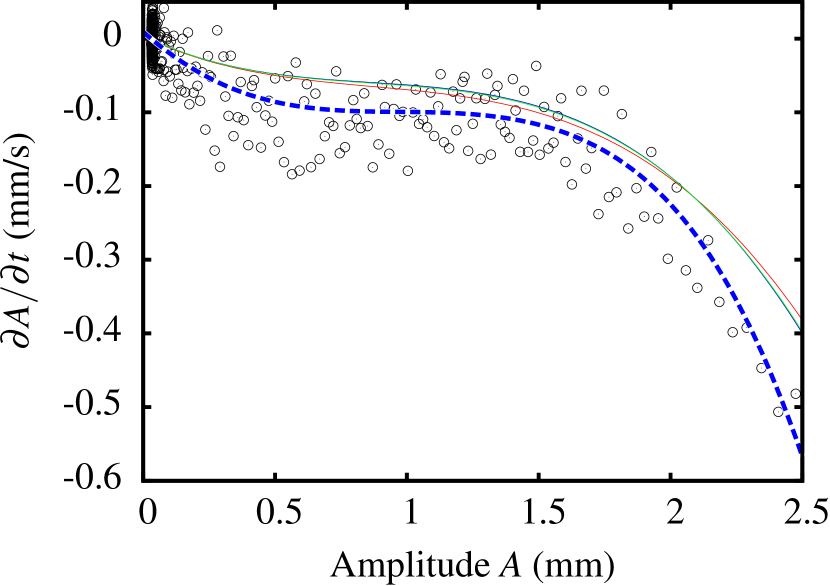
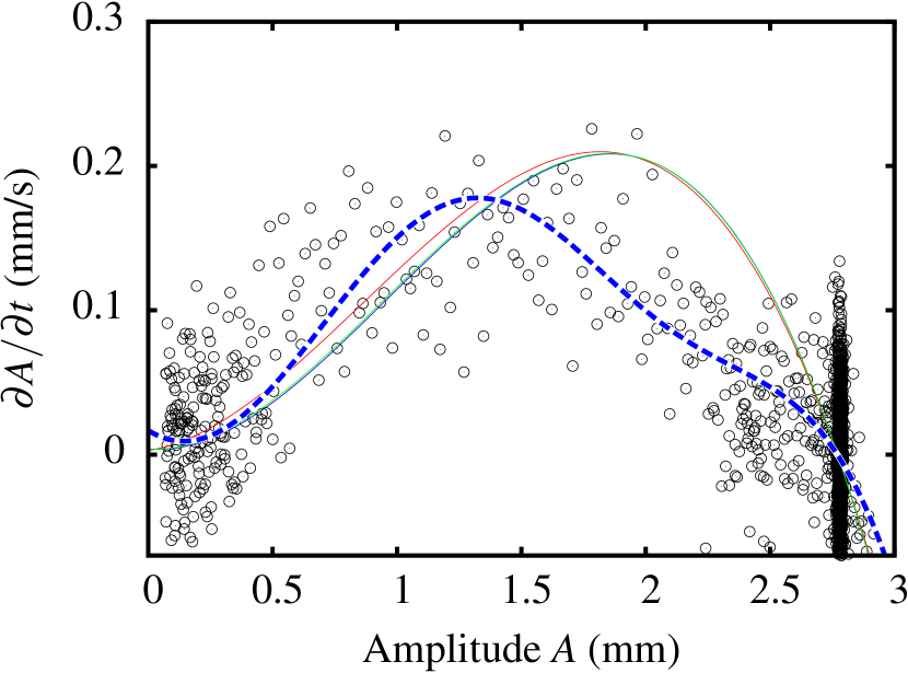
Even though the equilibrium curve can be represented reasonably well by at least the augmented amplitude equation, the fitted models all deviate from the measured data off the equilibrium curve in two ways. At small inductions, the model equations underestimate the velocity of the pattern decay. Figure 11(a) depicts the amplitude equations for an undercritical induction of $B=10.80\,\mathrm{mT}$. Here, the model equations all yield approximately the same result, but the difference to the measured data is roughly $30\,\%$. At overcritical inductions (figure 11b), the model equations culminate around $A=2$mm, while the RBF-approximation has its maximum around 1.5 mm, which coincides with the experimental observation.

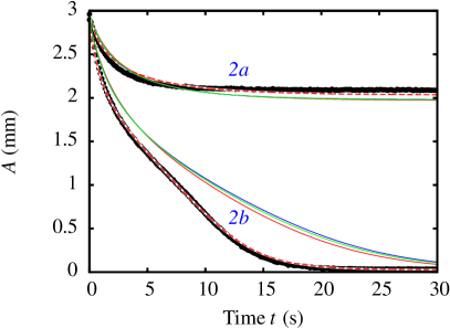
The quality of the theoretical descriptions becomes especially apparent when comparing the temporal evolution of the amplitude with numerical solutions of the amplitude equations, as shown in figure 12. These solutions are obtained by solving for $A$ in equations (1,2,12), with the first experimental data point as the initial condition. The solutions in the bistable regime (path 2a) describe the relaxation well, whereas the path 2b, observed at lower induction, differs notably from the integrated solution. This difference results from the underestimation of the decay rate far from the critical point, which was discussed above. Of course, the model equations are expansions about the critical point, and are not expected to be accurate far from the critical induction. In contrast, the temporal relaxation obtained from the RBF network fits the experimental data well for both paths.

A quantitative measure for the deviations of the model equations $s(\boldsymbol{x}_{j})$ from the experimental data $f(\boldsymbol{x}_{j})$ is given by the sum of squared residuals

$$\hat{\chi}^{2}=\sum_{j}\left|s(\boldsymbol{x}_{j})-f(\boldsymbol{x}_{j})\right|^{2}.$$ (14)

For the computation of $\hat{\chi}^{2}$, the dynamic evolution of the amplitudes in the whole range of the control parameter has been taken into account. The resulting values of $\hat{\chi}^{2}$ are listed in the 8th column of table 2. The values obtained for the equations (1,2,12) are larger than the one obtained for the RBF approximation. This indicates, that the dynamics away from the equilibrium curve is better described by the latter approximation. Note that in contrast to $\aleph$, $\hat{\chi}^{2}$ cannot discriminate between the different model equations  (1,2, 12).

For the overcritical induction, also the RBF approximation shows artefacts, as can be seen in figure 11(b). The measured data suggest a smooth shape of the amplitude equation, while the RBF approximation shows a bump near $A=2\dots 2.5\,\mathrm{mm}$. This irregularity stems from the double equilibrium point, which can be seen in figure 6 (c.f. traces 2a and 3a) and figure 7. These double equilibrium points represent similar, but different stable patterns and exist also in the neighbourhood of the data shown in figure 11(b). They influence the RBF network, because it is a global approximation scheme.

6 Discussion and Outlook

Using a highly viscous ferrofluid, the pattern evolution in the succession of the Rosensweig instability can be slowed down to the order of minutes. Therefore, it is possible to conveniently observe the dynamics using a two-dimensional imaging technique based on the absorption of X-rays. We have explored the full phase space in the vicinity of a hysteresis loop formed by a transcritical bifurcation and a saddle-node. From the measured data we have reconstructed a nonlinear equation of motion. A smooth approximation of the noisy experimental data with radial basis functions (RBF) provides an estimate for missing data and for the static amplitude. Amplitude equations for the instability were successfully fitted to the experimental data. The estimate of the equilibrium curve based on the cubic amplitude equation, as derived by bohlius2008amplitude, can be significantly improved by augmenting the quadratic coefficient with the factor $\left(1+\varepsilon\right)$. This factor can be extracted from the free energy functional of friedrichs2001 and reduces the deviation $\aleph$ between the equilibrium curve and the RBF reference by a factor of three.

However, a comparison of the absolute magnitude of both amplitude equations with the experimental data at an induction $5\,\%$ below the critical induction $B_{c}$ reveals, that neither amplitude equation can exactly describe all of the recorded dynamics. At least the agreement between the experiment and the model equations is within $30\,\%$. This is surprising, when considering that these equations are low order expansions about the critical threshold $B_{c}$, while the investigated range of about $7.5\,\%$ of $B_{c}$ even includes another critical point at a saddle node.

So far, the experimentally determined expansion coefficients can not sensibly be compared with the ones derived by theory, because the latter does not include a nonlinear magnetisation curve, which has a major influence on the instability. For example, for our fluid the critical threshold $B_{c}$ is shifted by about $10\%$. The change of the expansion coefficients is unknown. Its calculation remains a challenge for theory.

While we have extracted a nonlinear equation of motion for the specific example of the Rosensweig instability, it seems worth mentioning that the method is applicable to a wide set of overdamped pattern forming systems. A necessary precondition is that the control parameter can be switched much faster than the characteristic relaxation time.

In this paper only space filling homogeneous patterns have been considered for the method. However, the real system has additional degrees of freedom, which are manifested in the formation of localized states as observed previously by richter2005. Whereas in the latter work a local disturbance of the magnetic induction was needed to ignite localized states, here localized spikes and hexagonal patches emerge spontaneously when the measurement protocol pushes the system into the neighbourhood of the unstable branch. While a nuisance for the particular task of this paper, this multistability of hexagonal patches is an interesting phenomenon in itself, and may be seen in connection with homoclinic snaking lloyd2008lhpsee e.g.. However, for a clear picture further measurements are needed.

References

- [1] \harvarditemAbramowitz \harvardand Stegun1965abramowitz1970 Abramowitz M \harvardand Stegun I 1965 Handbook of mathematical functions: with formulas, graphs, and mathematical tables 9 edn Courier Dover Publications.
- [2] \harvarditemAristotle350 B.C.aristotle350 Aristotle 350 B.C. Physics Athens.
- [3] \harvarditemBohlius et al.2008bohlius2008amplitude Bohlius S, Brand H R \harvardand Pleiner H 2008 Prog. Theor. Phys. Supp. 175, 27.
- [4] \harvarditemBohlius et al.2007bohlius2007adjoint Bohlius S, Pleiner H \harvardand Brand H R 2007 Phys. Fluids 19, 094103.
- [5] \harvarditemCowley \harvardand Rosensweig1967cowley1967 Cowley M D \harvardand Rosensweig R E 1967 J. Fluid Mech. 30, 671.
- [6] \harvarditemCross \harvardand Hohenberg1993cross1993 Cross M C \harvardand Hohenberg P C 1993 Rev. Mod. Phys. 65, 851.
- [7] \harvarditemFriedrichs \harvardand Engel2001friedrichs2001 Friedrichs R \harvardand Engel A 2001 Phys. Rev. E 64, 021406.
- [8] \harvarditemGailitis1977gailitis1977 Gailitis A 1977 J. Fluid Mech. 82, 401.
- [9] \harvarditemGalilei1638galileo1638 Galilei G 1638 Discorsi e dimostrazioni matematiche Elsevier Leiden.
- [10] \harvarditemGollwitzer et al.2007gollwitzer2007 Gollwitzer C, Matthies G, Richter R, Rehberg I \harvardand Tobiska L 2007 J. Fluid Mech. 571, 455.
- [11] \harvarditemGollwitzer et al.2006gollwitzer2006b Gollwitzer C, Rehberg I \harvardand Richter R 2006 J. Phys.: Condens. Matter 18, 2643.
- [12] \harvarditemGollwitzer et al.2009gollwitzer2009nfi Gollwitzer C, Spyropoulos A N, Papathanasiou A G, Boudouvis A G \harvardand Richter R 2009 New Journal of Physics 11, 053016.
- [13] \harvarditemGreen \harvardand Silverman1994green1994nonparametric Green P \harvardand Silverman B 1994 Nonparametric regression and generalized linear models: a roughness penalty approach Chapman & Hall/CRC.
- [14] \harvarditemHardy1990hardy1990rbf Hardy R 1990 Computers & Mathematics with Applications 19, 163.
- [15] \harvarditemIvanov \harvardand Kuznetsova2001ivanov2001 Ivanov A O \harvardand Kuznetsova O B 2001 Phys. Rev. E 64, 041405.
- [16] \harvarditemKnieling et al.2010knieling2010 Knieling H, Rehberg I \harvardand Richter R 2010 J. Magn. Magn. Mater., submitted.
- [17] \harvarditemKnieling et al.2007knieling2007pre Knieling H, Richter R, Rehberg I, Matthies G \harvardand Lange A 2007 Phys. Rev. E 76, 66301.
- [18] \harvarditemKuznetsov \harvardand Spektor1976kuznetsov1976b Kuznetsov E A \harvardand Spektor M D 1976 Sov. Phys. JETP 44, 136.
- [19] \harvarditemLange2001lange2001b Lange A 2001 Europhys. Lett. 55(5), 327.
- [20] \harvarditemLange2002lange2002adjoint Lange A 2002 Int. J. Modern Phys. B 16, 1155.
- [21] \harvarditemLange et al.2000lange2000 Lange A, Reimann B \harvardand Richter R 2000 Phys. Rev. E 61, 5528.
- [22] \harvarditemLange et al.2001lange2001 Lange A, Reimann B \harvardand Richter R 2001 Magnetohydrodynamics 37, 261.
- [23] \harvarditemLloyd et al.2008lloyd2008lhp Lloyd D, Sandstede B, Avitabile D \harvardand Champneys A 2008 SIAM J. Appl. Dyn. Syst 7(3), 1049.
- [24] \harvarditemNeumaier1998neumaier1998regularization Neumaier A 1998 SIAM Review 40, 636.
- [25] \harvarditemNewton1687newton1687 Newton I 1687 Philosophiae naturalis principia mathematica Royal Society London.
- [26] \harvarditemPicard \harvardand Cook1984picard1984gcv Picard R R \harvardand Cook R D 1984 J. Am. Stat. Assoc 79, 575.
- [27] \harvarditemPowell1990powell1990rbftheory Powell M J D 1990 Vol. 2 of Advances in Numerical Analysis Oxford University Press pp. 105.
- [28] \harvarditemRault2000rault2000vogelfulcher Rault J 2000 Journal of Non-Crystalline Solids 271, 177.
- [29] \harvarditemReimann et al.2005reimann2005 Reimann B, Richter R, Knieling H \harvardand Rehberg I 2005 Phys. Rev. E 71, 055202(R).
- [30] \harvarditemRichter \harvardand Barashenkov2005richter2005 Richter R \harvardand Barashenkov I 2005 Phys. Rev. Lett. 94, 184503.
- [31] \harvarditemRichter \harvardand Bläsing2001richter2001 Richter R \harvardand Bläsing J 2001 Rev. Sci. Instrum. 72, 1729.
- [32] \harvarditemRosensweig1985rosensweig1985 Rosensweig R E 1985 Ferrohydrodynamics Cambridge University Press Cambridge, New York, Melbourne.
- [33] \harvarditemSalin1993salin1993 Salin D 1993 Europhys. Lett. 21, 667.
- [34] \harvarditemWeilepp \harvardand Brand1996weilepp1996 Weilepp J \harvardand Brand H R 1996 J. Phys. II France 6, 419.
- [35] \harvarditemWesfreid et al.1978wesfreid1978 Wesfreid J, Pomeau Y, Dubois M, Normand C \harvardand Bergé P 1978 J. Phys. Lett. Paris 39, 725.