โ€œIf the proof is correct, then no other recognition is neededโ€

by Grigori Y. Perelman

On the homotopy multiple-variable method
and its applications in the interactions
of nonlinear gravity waves

Shi-Jun LIAO

State Key Laboratory of Ocean Engineering

School of Naval Architecture, Ocean and Civil Engineering

Shanghai Jiao Tong University, Shanghai 200240, China

( Email address: sjliao@sjtu.edu.cn )

Abstract The basic ideas of a homotopy-based multiple-variable method is proposed and applied to investigate the nonlinear interactions of periodic traveling waves. Mathematically, this method does not depend upon any small physical parameters at all and thus is more general than the traditional multiple-scale perturbation techniques. Physically, it is found that, for a fully developed wave system, the amplitudes of all wave components are finite even if the wave resonance condition given by Phillips (1960) is exactly satisfied. Besides, it is revealed that there exist multiple resonant waves, and that the amplitudes of resonant wave may be much smaller than those of primary waves so that the resonant waves sometimes contain rather small part of wave energy. Furthermore, a wave resonance condition for arbitrary numbers of traveling waves with large wave amplitudes is given, which logically contains Phillipsโ€™ four-wave resonance condition but opens a way to investigate the strongly nonlinear interaction of more than four traveling waves with large amplitudes. This work also illustrates that the homotopy multiple-variable method is helpful to gain solutions with important physical meanings of nonlinear problems, if the multiple variables are properly defined with clear physical meanings.

Key Words nonlinearity, wave resonance, multiple-variable, HAM

1 Introduction

In his pioneering work about nonlinear interaction of four gravity waves in deep water, Phillips [1] gave the criterion condition for wave resonance

๐ค1ยฑ๐ค2ยฑ๐ค3ยฑ๐ค4=0,ฯƒ1ยฑฯƒ2ยฑฯƒ3ยฑฯƒ4=0,formulae-sequenceplus-or-minussubscript๐ค1subscript๐ค2subscript๐ค3subscript๐ค40plus-or-minussubscript๐œŽ1subscript๐œŽ2subscript๐œŽ3subscript๐œŽ40{\bf k}_{1}\pm{\bf k}_{2}\pm{\bf k}_{3}\pm{\bf k}_{4}=0,\;\;\;\sigma_{1}\pm\sigma_{2}\pm\sigma_{3}\pm\sigma_{4}=0, (1)

where ฯƒi=gโ€‹kisubscript๐œŽ๐‘–๐‘”subscript๐‘˜๐‘–\sigma_{i}=\sqrt{gk_{i}} with ki=|๐คi|subscript๐‘˜๐‘–subscript๐ค๐‘–k_{i}=|{\bf k}_{i}| (i=1,2,3,4๐‘–1234i=1,2,3,4) is the wave angular frequency, and ๐คisubscript๐ค๐‘–{\bf k}_{i} denotes the wave number. Note that, Phillips resonance condition (1) works only for weakly nonlinear waves with small amplitudes, because ฯƒi=gโ€‹kisubscript๐œŽ๐‘–๐‘”subscript๐‘˜๐‘–\sigma_{i}=\sqrt{gk_{i}} is the angular frequency of linear theory for a single gravity wave with small amplitude.

Especially, in case of ๐ค4=๐ค1subscript๐ค4subscript๐ค1{\bf k}_{4}={\bf k}_{1}, Phillips [1] showed that, if ๐ค3=2โ€‹๐ค1โˆ’๐ค๐Ÿsubscript๐ค32subscript๐ค1subscript๐ค2{\bf k}_{3}=2{\bf k}_{1}-{\bf k_{2}} and ฯƒ3=2โ€‹ฯƒ1โˆ’ฯƒ2subscript๐œŽ32subscript๐œŽ1subscript๐œŽ2\sigma_{3}=2\sigma_{1}-\sigma_{2}, then a steady-state solution for the triad did not exist, and the amplitude of the third wave, if initially zero, would grow linearly in time. This conclusion was confirmed by Longuet-Higgins [2] via perturbation theory and supported by some experiments [3, 4]. Besides, Benney [5] solved the equations governing the time dependence of the resonant modes and studied the energy-sharing mechanism involved.

Although half century passed since Phillipsโ€™ pioneering work [1], there exist still some open questions about nonlinear interaction between gravity waves. First, Bretherton [6] pointed out that the perturbation scheme used by Phillips breaks down for large time, and suggested by investigating a one-dimensional dispersive wave model that the amplitude of each wave component should be bounded. Are the amplitudes of each component waves bounded when the resonance condition is exactly satisfied? Besides, based on perturbation method, Phillips [1] gave the condition (1) of wave resonance for only four waves. What is the resonance condition for more waves with large amplitude? It seems difficult to apply the perturbation scheme used by Phillips [1] and Longuet-Higgins [2] to answer these questions, because the related algebra was daunting and โ€œextraordinarily tediousโ€, as mentioned by Phillips [7].

Perturbation techniques are powerful analytic tools for nonlinear equations, especially when there indeed exists a small physical parameter, i.e. perturbation quantity: the solution is often expressed in a series of the small physical parameter, and the original nonlinear equation is transformed into a sequence of (mostly linear) sub-problems. Frankly speaking, perturbation techniques greatly enrich our knowledge and deepen our understandings about many nonlinear problems. It has a golden times before the times of computer when people calculated mostly by hand and wrote the โ€œanalyticโ€ results on one page (or a few pages) of paper. However, some restrictions of perturbation techniques are well-known. First of all, it depends too strongly on the small physical parameters, but unfortunately many nonlinear problems have no such kind of small parameters. Besides, perturbation approximations often break down when the so-called perturbation quantity increases. All of these disadvantages greatly restrict the applications of perturbation techniques.

In history, the calculating tools have a deep impression on the mathematical methods. One example is the development of numerical methods such as the finite element method, the finite difference method, and so on. Fortunately, we are now in the times of computer: a computer can do more than 1017superscript101710^{17} fundamental operations and save a great lot of data in diskette within a seconds! Besides, there are some powerful symbolic computation software such as Maple, Mathematica, MathLab and so on. Today, using these software on a laptop, one can deduce lengthy formulas, calculate a rather complicated expression, and save analytic results on diskette in a seconds which might be hundreds of papers long if printed out. So, when the pencil and paper are replaced by the keyboard, diskette and CPU of a personal computer, the revolution of analytic approximation methods comes, although it is much later than the revolution of numerical approximation methods.

What kind of analytic approximation methods should we have in the times of computer? Can we overcome the restrictions of the traditional perturbation methods? The answer is rather positive and stimulant. Note that, the traditional concept of โ€œanalyticโ€ solution came into being in the times of pen and paper, and it was traditionally believed that a โ€œanalyticโ€ result must be short and should be written on less than one paper. Today, it needs only a few seconds to save a rather complicated formula in diskette which might be even more than hundreds of papers. Besides, one needs only a few seconds to calculate such a lengthy expression by a personal computer. In fact, one spends much less time to save and calculate such lengthy formula by computer than to calculate and write a simple formula with half-page length by hand. Therefore, in the times of computer, the concept of โ€œanalyticโ€ result must be modified, and an โ€œanalyticโ€ formula can be very lengthy. Secondly, due to the high performance of symbolic computation of a computer, it should be easy to obtain high-order approximations by means of the new analytic methods. And more importantly, some efficient approaches should be provided to ensure the high accuracy of analytic approximations even for strongly nonlinear problems. In a short, the new analytic method should belong to the times of computer, and besides should overcome the restrictions of traditional methods mentioned above.

Such a kind of analytic method has been developed in 1990s when the early symbolic computation software just appeared: based on the homotopy, a fundamental concept in topology, the homotopy analysis method (HAM) was first proposed by Liao [8, 9, 10, 11, 12, 13, 14, 15, 16]. Different from perturbation methods, the HAM has nothing to do with any physical parameters. More importantly, different from other previous analytic methods, the HAM provides us a simple way to ensure the convergence of solution series. Besides, it has been proved that the HAM logically contains the previous non-perturbation methods such as Lyapunov artificial small parameter method, Adomian decomposition method, the ฮด๐›ฟ\delta-expansion method and so on. Therefore, the HAM is valid for strongly nonlinear problems and thus is more general. The HAM has been successfully applied to solve different types of nonlinear ODEs and PDEs in science and finance.

The idea of multiple-scales of perturbation methods has clear physical meanings. In this article, based on the homotopy analysis method (HAM), we propose a multiple-variable technique for general nonlinear differential equations, which keeps the clear physical meaning of multiple-scales but abandons completely the small physical parameters of perturbation techniques. In ยง2, the nonlinear interaction of primary periodic traveling waves in deep water is used as an example to describe the basic ideas of this approach. In ยง3, we give convergent series solution of a fully developed system of two primary waves even when Phillipsโ€™ resonance condition is exactly satisfied. Besides, some interesting results related to multiple resonant waves are reported. Especially, we reveal that Phillips resonance wave condition is mathematically equivalent to the zero eigenvalue of the eigenfunction related to the resonant wave. In ยง4.1, the expression of the eigenvalue of a fully developed wave system for arbitrary number of traveling waves is derived, and then a resonance condition for arbitrary number of small-amplitude waves is given. In ยง4.2, a more general resonance condition is further obtained from the physical points of view, which logically contains Phillipsโ€™ resonance condition (1) but works for arbitrary number of traveling waves with large amplitudes. In ยง5, the concluding remarks, open questions and discussions are given. The detailed mathematical derivation is given in Appendix A, and the proof of a convergence theorem is given briefly in Appendix B.

2 Mathematical description

Let z๐‘งz denote the vertical co-ordinate, x,y๐‘ฅ๐‘ฆx,y the horizontal co-ordinates, t๐‘กt the time, z=ฮถโ€‹(x,y,t)๐‘ง๐œ๐‘ฅ๐‘ฆ๐‘กz=\zeta(x,y,t) the free surface, respectively. The three axises of x,y,z๐‘ฅ๐‘ฆ๐‘งx,y,z are perpendicular to each other, with the unit vector ๐ข,๐ฃ,๐ค๐ข๐ฃ๐ค{\bf i},{\bf j},{\bf k}, respectively, i.e. ๐ขโ‹…๐ฃ=๐ขโ‹…๐ค=๐ฃโ‹…๐ค=0โ‹…๐ข๐ฃโ‹…๐ข๐คโ‹…๐ฃ๐ค0{\bf i}\cdot{\bf j}={\bf i}\cdot{\bf k}={\bf j}\cdot{\bf k}=0, where โ‹…โ‹…\cdot is the multiplication dot. Assume that the vorticity is negligible and there exists a potential ฯ†โ€‹(x,y,z,t)๐œ‘๐‘ฅ๐‘ฆ๐‘ง๐‘ก\varphi(x,y,z,t) for the velocity ๐ฎ๐ฎ\bf u that ๐ฎ=โˆ‡ฯ†๐ฎโˆ‡๐œ‘{\bf u}=\nabla\varphi and

โˆ‡2ฯ†=0,zโ‰คฮถโ€‹(x,y,t)formulae-sequencesuperscriptโˆ‡2๐œ‘0๐‘ง๐œ๐‘ฅ๐‘ฆ๐‘ก\nabla^{2}\varphi=0,\;\;\;z\leq\zeta(x,y,t) (2)

in an incompressible flow, where

โˆ‡=๐ขโ€‹โˆ‚โˆ‚x+๐ฃโ€‹โˆ‚โˆ‚y+๐คโ€‹โˆ‚โˆ‚z.โˆ‡๐ข๐‘ฅ๐ฃ๐‘ฆ๐ค๐‘ง\nabla={\bf i}\frac{\partial}{\partial x}+{\bf j}\frac{\partial}{\partial y}+{\bf k}\frac{\partial}{\partial z}.

On the free surface z=ฮถโ€‹(x,y,t)๐‘ง๐œ๐‘ฅ๐‘ฆ๐‘กz=\zeta(x,y,t), the pressure is constant, which gives from Bernoulliโ€™s equation the dynamic boundary condition

gโ€‹ฮถ+โˆ‚ฯ†โˆ‚t+12โ€‹๐ฎ2=0,onย z=ฮถโ€‹(x,y,t),๐‘”๐œ๐œ‘๐‘ก12superscript๐ฎ20onย z=ฮถ(x,y,t)g\;\zeta+\frac{\partial\varphi}{\partial t}+\frac{1}{2}{\bf u}^{2}=0,\;\;\;\mbox{on $z=\zeta(x,y,t)$}, (3)

where g๐‘”g is the acceleration due to gravity. Besides, zโˆ’ฮถ๐‘ง๐œz-\zeta vanishes following a particle, which gives the kinematic boundary condition

โˆ‚ฮถโˆ‚tโˆ’โˆ‚ฯ†โˆ‚z+(โˆ‚ฯ†โˆ‚xโ€‹โˆ‚ฮถโˆ‚x+โˆ‚ฯ†โˆ‚yโ€‹โˆ‚ฮถโˆ‚y)=0,onย z=ฮถโ€‹(x,y,t).๐œ๐‘ก๐œ‘๐‘ง๐œ‘๐‘ฅ๐œ๐‘ฅ๐œ‘๐‘ฆ๐œ๐‘ฆ0onย z=ฮถ(x,y,t)\frac{\partial\zeta}{\partial t}-\frac{\partial\varphi}{\partial z}+\left(\frac{\partial\varphi}{\partial x}\frac{\partial\zeta}{\partial x}+\frac{\partial\varphi}{\partial y}\frac{\partial\zeta}{\partial y}\right)=0,\;\;\;\mbox{on $z=\zeta(x,y,t)$}. (4)

Combining the above two equations gives the boundary condition

โˆ‚2ฯ†โˆ‚t2+gโ€‹โˆ‚ฯ†โˆ‚z+โˆ‚(๐ฎ2)โˆ‚t+๐ฎโ‹…โˆ‡(12โ€‹๐ฎ2)=0,onย z=ฮถโ€‹(x,y,t),superscript2๐œ‘superscript๐‘ก2๐‘”๐œ‘๐‘งsuperscript๐ฎ2๐‘กโ‹…๐ฎโˆ‡12superscript๐ฎ20onย z=ฮถ(x,y,t)\frac{\partial^{2}\varphi}{\partial t^{2}}+g\frac{\partial\varphi}{\partial z}+\frac{\partial({\bf u}^{2})}{\partial t}+{\bf u}\cdot\nabla\left(\frac{1}{2}{\bf u}^{2}\right)=0,\;\;\;\mbox{on $z=\zeta(x,y,t)$}, (5)

where ๐ฎ=โˆ‡ฯ†๐ฎโˆ‡๐œ‘{\bf u}=\nabla\varphi and ๐ฎ2=โˆ‡ฯ†โ‹…โˆ‡ฯ†superscript๐ฎ2โ‹…โˆ‡๐œ‘โˆ‡๐œ‘{\bf u}^{2}=\nabla\varphi\cdot\nabla\varphi. On the bottom, it holds

โˆ‚ฯ†โˆ‚z=0,asย zโ†’โˆ’โˆž.๐œ‘๐‘ง0asย zโ†’โˆ’โˆž\frac{\partial\varphi}{\partial z}=0,\;\;\;\mbox{as $z\rightarrow-\infty$}. (6)

For details, please refer to Phillips [1] and Longuet-Higgins [2] .

Without loss of generality, let us first consider a wave system basically composed of two trains of primary traveling gravity waves in deep water with wave numbers ๐ค1,๐ค2subscript๐ค1subscript๐ค2{\bf k}_{1},{\bf k}_{2} and the corresponding angular frequencies ฯƒ1,ฯƒ2subscript๐œŽ1subscript๐œŽ2\sigma_{1},\sigma_{2}, respectively, where ๐ค1ร—๐ค2โ‰ 0subscript๐ค1subscript๐ค20{\bf k}_{1}\times{\bf k}_{2}\neq 0 (i.e. the two traveling waves are not collinear). Due to nonlinear interaction, this wave system contains an infinite number of wave components with the corresponding wave number mโ€‹๐ค1+nโ€‹๐ค2๐‘šsubscript๐ค1๐‘›subscript๐ค2m{\bf k}_{1}+n{\bf k}_{2}, where m,n๐‘š๐‘›m,n are integers. Assume that the wave system is in equilibrium so that each wave amplitude is constant, i.e. independent of the time. Let ฮฑ1,ฮฑ2subscript๐›ผ1subscript๐›ผ2\alpha_{1},\alpha_{2} denote the angles between the positive x๐‘ฅx-axis ๐ข๐ข{\bf i} and the wave number vectors ๐ค1subscript๐ค1{\bf k}_{1} and ๐ค2subscript๐ค2{\bf k}_{2}, respectively, where ๐ค1โ‹…๐ค=๐ค2โ‹…๐ค=0โ‹…subscript๐ค1๐คโ‹…subscript๐ค2๐ค0{\bf k}_{1}\cdot{\bf k}={\bf k}_{2}\cdot{\bf k}=0, i.e. the z๐‘งz-axis is perpendicular to the wave numbers ๐ค1,๐ค2subscript๐ค1subscript๐ค2{\bf k}_{1},{\bf k}_{2}. Then,

๐ค1subscript๐ค1\displaystyle{\bf k}_{1} =\displaystyle= k1โ€‹(cosโกฮฑ1โ€‹๐ข+sinโกฮฑ1โ€‹๐ฃ),subscript๐‘˜1subscript๐›ผ1๐ขsubscript๐›ผ1๐ฃ\displaystyle k_{1}\;\left(\cos\alpha_{1}\;{\bf i}+\sin\alpha_{1}\;{\bf j}\right), (7)
๐ค2subscript๐ค2\displaystyle{\bf k}_{2} =\displaystyle= k2โ€‹(cosโกฮฑ2โ€‹๐ข+sinโกฮฑ2โ€‹๐ฃ),subscript๐‘˜2subscript๐›ผ2๐ขsubscript๐›ผ2๐ฃ\displaystyle k_{2}\;\left(\cos\alpha_{2}\;{\bf i}+\sin\alpha_{2}\;{\bf j}\right), (8)

where k1=|๐ค1|subscript๐‘˜1subscript๐ค1k_{1}=|{\bf k}_{1}| and k2=|๐ค2|subscript๐‘˜2subscript๐ค2k_{2}=|{\bf k}_{2}|.

Write ๐ซ=xโ€‹๐ข+yโ€‹๐ฃ๐ซ๐‘ฅ๐ข๐‘ฆ๐ฃ{\bf r}=x{\bf i}+y{\bf j}. According to linear gravity wave theory, the two trains of primary waves traveling with the wave numbers ๐ค1subscript๐ค1{\bf k}_{1} and ๐ค2subscript๐ค2{\bf k}_{2} are given by a1โ€‹cosโกฮพ1,a2โ€‹cosโกฮพ2,subscript๐‘Ž1subscript๐œ‰1subscript๐‘Ž2subscript๐œ‰2a_{1}\cos\xi_{1},\;a_{2}\cos\xi_{2}, respectively, where

ฮพ1subscript๐œ‰1\displaystyle\xi_{1} =\displaystyle= ๐ค1โ‹…๐ซโˆ’ฯƒ1โ€‹t=k1โ€‹cosโกฮฑ1โ€‹x+k1โ€‹sinโกฮฑ1โ€‹yโˆ’ฯƒ1โ€‹tโ‹…subscript๐ค1๐ซsubscript๐œŽ1๐‘กsubscript๐‘˜1subscript๐›ผ1๐‘ฅsubscript๐‘˜1subscript๐›ผ1๐‘ฆsubscript๐œŽ1๐‘ก\displaystyle{\bf k}_{1}\cdot{\bf r}-\sigma_{1}\;t=k_{1}\cos\alpha_{1}\;x+k_{1}\sin\alpha_{1}\;y-\sigma_{1}\;t (9)
ฮพ2subscript๐œ‰2\displaystyle\xi_{2} =\displaystyle= ๐ค2โ‹…๐ซโˆ’ฯƒ2โ€‹t=k2โ€‹cosโกฮฑ2โ€‹x+k2โ€‹sinโกฮฑ2โ€‹yโˆ’ฯƒ2โ€‹t.โ‹…subscript๐ค2๐ซsubscript๐œŽ2๐‘กsubscript๐‘˜2subscript๐›ผ2๐‘ฅsubscript๐‘˜2subscript๐›ผ2๐‘ฆsubscript๐œŽ2๐‘ก\displaystyle{\bf k}_{2}\cdot{\bf r}-\sigma_{2}\;t=k_{2}\cos\alpha_{2}\;x+k_{2}\sin\alpha_{2}\;y-\sigma_{2}\;t. (10)

So, the above two variables have very clear physical meaning: for the considered problem, the wave profile must be a periodic function of ฮพ1subscript๐œ‰1\xi_{1} and ฮพ2subscript๐œ‰2\xi_{2}. Mathematically, using these two variables, the time t๐‘กt should not appear explicitly for a fully develop wave system. In other words, one can express the potential function ฯ†โ€‹(x,y,z,t)=ฯ•โ€‹(ฮพ1,ฮพ2,z)๐œ‘๐‘ฅ๐‘ฆ๐‘ง๐‘กitalic-ฯ•subscript๐œ‰1subscript๐œ‰2๐‘ง\varphi(x,y,z,t)=\phi(\xi_{1},\xi_{2},z) and the wave surface ฮถโ€‹(x,y,t)=ฮทโ€‹(ฮพ1,ฮพ2)๐œ๐‘ฅ๐‘ฆ๐‘ก๐œ‚subscript๐œ‰1subscript๐œ‰2\zeta(x,y,t)=\eta(\xi_{1},\xi_{2}) for two trains of primary traveling waves. In this way, the mathematical expressions of the unknown potential function and wave surface are clear, with clear physical meanings.

Obviously, it holds

โˆ‚ฯ†โˆ‚x=โˆ‚ฯ•โˆ‚ฮพ1โ€‹โˆ‚ฮพ1โˆ‚x+โˆ‚ฯ•โˆ‚ฮพ2โ€‹โˆ‚ฮพ2โˆ‚x=(k1โ€‹cosโกฮฑ1)โ€‹โˆ‚ฯ•โˆ‚ฮพ1+(k2โ€‹cosโกฮฑ2)โ€‹โˆ‚ฯ•โˆ‚ฮพ2,๐œ‘๐‘ฅitalic-ฯ•subscript๐œ‰1subscript๐œ‰1๐‘ฅitalic-ฯ•subscript๐œ‰2subscript๐œ‰2๐‘ฅsubscript๐‘˜1subscript๐›ผ1italic-ฯ•subscript๐œ‰1subscript๐‘˜2subscript๐›ผ2italic-ฯ•subscript๐œ‰2\frac{\partial\varphi}{\partial x}=\frac{\partial\phi}{\partial\xi_{1}}\frac{\partial\xi_{1}}{\partial x}+\frac{\partial\phi}{\partial\xi_{2}}\frac{\partial\xi_{2}}{\partial x}=\left(k_{1}\cos\alpha_{1}\right)\frac{\partial\phi}{\partial\xi_{1}}+\left(k_{2}\cos\alpha_{2}\right)\frac{\partial\phi}{\partial\xi_{2}},

and similarly

โˆ‚ฯ†โˆ‚y๐œ‘๐‘ฆ\displaystyle\frac{\partial\varphi}{\partial y} =\displaystyle= (k1โ€‹sinโกฮฑ1)โ€‹โˆ‚ฯ•โˆ‚ฮพ1+(k2โ€‹sinโกฮฑ2)โ€‹โˆ‚ฯ•โˆ‚ฮพ2,subscript๐‘˜1subscript๐›ผ1italic-ฯ•subscript๐œ‰1subscript๐‘˜2subscript๐›ผ2italic-ฯ•subscript๐œ‰2\displaystyle\left(k_{1}\sin\alpha_{1}\right)\frac{\partial\phi}{\partial\xi_{1}}+\left(k_{2}\sin\alpha_{2}\right)\frac{\partial\phi}{\partial\xi_{2}},
โˆ‚ฯ†โˆ‚z๐œ‘๐‘ง\displaystyle\frac{\partial\varphi}{\partial z} =\displaystyle= โˆ‚ฯ•โˆ‚z,italic-ฯ•๐‘ง\displaystyle\frac{\partial\phi}{\partial z},
โˆ‚ฯ†โˆ‚t๐œ‘๐‘ก\displaystyle\frac{\partial\varphi}{\partial t} =\displaystyle= โˆ’ฯƒ1โ€‹โˆ‚ฯ•โˆ‚ฮพ1โˆ’ฯƒ2โ€‹โˆ‚ฯ•โˆ‚ฮพ2,subscript๐œŽ1italic-ฯ•subscript๐œ‰1subscript๐œŽ2italic-ฯ•subscript๐œ‰2\displaystyle-\sigma_{1}\frac{\partial\phi}{\partial\xi_{1}}-\sigma_{2}\frac{\partial\phi}{\partial\xi_{2}},
โˆ‚2ฯ†โˆ‚t2superscript2๐œ‘superscript๐‘ก2\displaystyle\frac{\partial^{2}\varphi}{\partial t^{2}} =\displaystyle= ฯƒ12โ€‹โˆ‚2ฯ•โˆ‚ฮพ12+2โ€‹ฯƒ1โ€‹ฯƒ2โ€‹โˆ‚2ฯ•โˆ‚ฮพ1โ€‹โˆ‚ฮพ2+ฯƒ22โ€‹โˆ‚2ฯ•โˆ‚ฮพ22.superscriptsubscript๐œŽ12superscript2italic-ฯ•superscriptsubscript๐œ‰122subscript๐œŽ1subscript๐œŽ2superscript2italic-ฯ•subscript๐œ‰1subscript๐œ‰2superscriptsubscript๐œŽ22superscript2italic-ฯ•superscriptsubscript๐œ‰22\displaystyle\sigma_{1}^{2}\;\frac{\partial^{2}\phi}{\partial\xi_{1}^{2}}+2\sigma_{1}\sigma_{2}\;\frac{\partial^{2}\phi}{\partial\xi_{1}\partial\xi_{2}}+\sigma_{2}^{2}\;\frac{\partial^{2}\phi}{\partial\xi_{2}^{2}}.

Then,

โˆ‡ฯ†โˆ‡๐œ‘\displaystyle\nabla\varphi =\displaystyle= ๐ขโ€‹โˆ‚ฯ†โˆ‚x+๐ฃโ€‹โˆ‚ฯ†โˆ‚y+๐คโ€‹โˆ‚ฯ†โˆ‚z๐ข๐œ‘๐‘ฅ๐ฃ๐œ‘๐‘ฆ๐ค๐œ‘๐‘ง\displaystyle{\bf i}\frac{\partial\varphi}{\partial x}+{\bf j}\frac{\partial\varphi}{\partial y}+{\bf k}\frac{\partial\varphi}{\partial z} (11)
=\displaystyle= k1โ€‹(cosโกฮฑ1โ€‹๐ข+sinโกฮฑ1โ€‹๐ฃ)โ€‹โˆ‚ฯ•โˆ‚ฮพ1+k2โ€‹(cosโกฮฑ2โ€‹๐ข+sinโกฮฑ2โ€‹๐ฃ)โ€‹โˆ‚ฯ•โˆ‚ฮพ2+๐คโ€‹โˆ‚ฯ•โˆ‚zsubscript๐‘˜1subscript๐›ผ1๐ขsubscript๐›ผ1๐ฃitalic-ฯ•subscript๐œ‰1subscript๐‘˜2subscript๐›ผ2๐ขsubscript๐›ผ2๐ฃitalic-ฯ•subscript๐œ‰2๐คitalic-ฯ•๐‘ง\displaystyle k_{1}\;\left(\cos\alpha_{1}\;{\bf i}+\sin\alpha_{1}\;{\bf j}\right)\frac{\partial\phi}{\partial\xi_{1}}+k_{2}\;\left(\cos\alpha_{2}\;{\bf i}+\sin\alpha_{2}\;{\bf j}\right)\frac{\partial\phi}{\partial\xi_{2}}+{\bf k}\frac{\partial\phi}{\partial z}
=\displaystyle= ๐ค1โ€‹โˆ‚ฯ•โˆ‚ฮพ1+๐ค2โ€‹โˆ‚ฯ•โˆ‚ฮพ2+๐คโ€‹โˆ‚ฯ•โˆ‚z=โˆ‡^โ€‹ฯ•=๐ฎ,subscript๐ค1italic-ฯ•subscript๐œ‰1subscript๐ค2italic-ฯ•subscript๐œ‰2๐คitalic-ฯ•๐‘ง^โˆ‡italic-ฯ•๐ฎ\displaystyle{\bf k}_{1}\frac{\partial\phi}{\partial\xi_{1}}+{\bf k}_{2}\frac{\partial\phi}{\partial\xi_{2}}+{\bf k}\frac{\partial\phi}{\partial z}=\hat{\nabla}\phi={\bf u},

where

โˆ‡^=๐ค1โ€‹โˆ‚โˆ‚ฮพ1+๐ค2โ€‹โˆ‚โˆ‚ฮพ2+๐คโ€‹โˆ‚โˆ‚z.^โˆ‡subscript๐ค1subscript๐œ‰1subscript๐ค2subscript๐œ‰2๐ค๐‘ง\hat{\nabla}={\bf k}_{1}\frac{\partial}{\partial\xi_{1}}+{\bf k}_{2}\frac{\partial}{\partial\xi_{2}}+{\bf k}\frac{\partial}{\partial z}. (12)

Thus,

๐ฎ2superscript๐ฎ2\displaystyle{\bf u}^{2} =\displaystyle= โˆ‡ฯ†โ‹…โˆ‡ฯ†=โˆ‡^โ€‹ฯ•โ‹…โˆ‡^โ€‹ฯ•โ‹…โˆ‡๐œ‘โˆ‡๐œ‘โ‹…^โˆ‡italic-ฯ•^โˆ‡italic-ฯ•\displaystyle\nabla\varphi\cdot\nabla\varphi=\hat{\nabla}\phi\cdot\hat{\nabla}\phi (13)
=\displaystyle= k12โ€‹(โˆ‚ฯ•โˆ‚ฮพ1)2+2โ€‹๐ค1โ‹…๐ค2โ€‹โˆ‚ฯ•โˆ‚ฮพ1โ€‹โˆ‚ฯ•โˆ‚ฮพ2+k22โ€‹(โˆ‚ฯ•โˆ‚ฮพ2)2+(โˆ‚ฯ•โˆ‚z)2,superscriptsubscript๐‘˜12superscriptitalic-ฯ•subscript๐œ‰12โ‹…2subscript๐ค1subscript๐ค2italic-ฯ•subscript๐œ‰1italic-ฯ•subscript๐œ‰2superscriptsubscript๐‘˜22superscriptitalic-ฯ•subscript๐œ‰22superscriptitalic-ฯ•๐‘ง2\displaystyle k_{1}^{2}\left(\frac{\partial\phi}{\partial\xi_{1}}\right)^{2}+2{\bf k}_{1}\cdot{\bf k}_{2}\;\frac{\partial\phi}{\partial\xi_{1}}\frac{\partial\phi}{\partial\xi_{2}}+k_{2}^{2}\left(\frac{\partial\phi}{\partial\xi_{2}}\right)^{2}+\left(\frac{\partial\phi}{\partial z}\right)^{2},

where ๐ค1โ‹…๐ค=๐ค2โ‹…๐ค=0โ‹…subscript๐ค1๐คโ‹…subscript๐ค2๐ค0{\bf k}_{1}\cdot{\bf k}={\bf k}_{2}\cdot{\bf k}=0 is used, and

๐ค1โ‹…๐ค2=k1โ€‹k2โ€‹cosโก(ฮฑ1โˆ’ฮฑ2).โ‹…subscript๐ค1subscript๐ค2subscript๐‘˜1subscript๐‘˜2subscript๐›ผ1subscript๐›ผ2{\bf k}_{1}\cdot{\bf k}_{2}=k_{1}k_{2}\cos(\alpha_{1}-\alpha_{2}).

In general, it holds

โˆ‡^โ€‹ฯ•โ‹…โˆ‡^โ€‹ฯˆโ‹…^โˆ‡italic-ฯ•^โˆ‡๐œ“\displaystyle\hat{\nabla}\phi\cdot\hat{\nabla}\psi =\displaystyle= k12โ€‹โˆ‚ฯ•โˆ‚ฮพ1โ€‹โˆ‚ฯˆโˆ‚ฮพ1+๐ค1โ‹…๐ค2โ€‹(โˆ‚ฯ•โˆ‚ฮพ1โ€‹โˆ‚ฯˆโˆ‚ฮพ2+โˆ‚ฯˆโˆ‚ฮพ1โ€‹โˆ‚ฯ•โˆ‚ฮพ2)+k22โ€‹โˆ‚ฯ•โˆ‚ฮพ2โ€‹โˆ‚ฯˆโˆ‚ฮพ2+โˆ‚ฯ•โˆ‚zโ€‹โˆ‚ฯˆโˆ‚zsuperscriptsubscript๐‘˜12italic-ฯ•subscript๐œ‰1๐œ“subscript๐œ‰1โ‹…subscript๐ค1subscript๐ค2italic-ฯ•subscript๐œ‰1๐œ“subscript๐œ‰2๐œ“subscript๐œ‰1italic-ฯ•subscript๐œ‰2superscriptsubscript๐‘˜22italic-ฯ•subscript๐œ‰2๐œ“subscript๐œ‰2italic-ฯ•๐‘ง๐œ“๐‘ง\displaystyle k_{1}^{2}\;\frac{\partial\phi}{\partial\xi_{1}}\frac{\partial\psi}{\partial\xi_{1}}+{\bf k}_{1}\cdot{\bf k}_{2}\;\left(\frac{\partial\phi}{\partial\xi_{1}}\frac{\partial\psi}{\partial\xi_{2}}+\frac{\partial\psi}{\partial\xi_{1}}\frac{\partial\phi}{\partial\xi_{2}}\right)+k_{2}^{2}\;\frac{\partial\phi}{\partial\xi_{2}}\frac{\partial\psi}{\partial\xi_{2}}+\frac{\partial\phi}{\partial z}\frac{\partial\psi}{\partial z}\;\;\;\;\; (14)

for arbitrary functions ฯ•โ€‹(ฮพ1,ฮพ2,z)italic-ฯ•subscript๐œ‰1subscript๐œ‰2๐‘ง\phi(\xi_{1},\xi_{2},z) and ฯˆโ€‹(ฮพ1,ฮพ2,z)๐œ“subscript๐œ‰1subscript๐œ‰2๐‘ง\psi(\xi_{1},\xi_{2},z).

Similarly, we have

โˆ‡2ฯ†superscriptโˆ‡2๐œ‘\displaystyle\nabla^{2}\varphi =\displaystyle= โˆ‡^2โ€‹ฯ•=k12โ€‹โˆ‚2ฯ•โˆ‚ฮพ12+2โ€‹๐ค1โ‹…๐ค2โ€‹โˆ‚2ฯ•โˆ‚ฮพ1โ€‹โˆ‚ฮพ2+k22โ€‹โˆ‚2ฯ•โˆ‚ฮพ22+โˆ‚2ฯ•โˆ‚z2.superscript^โˆ‡2italic-ฯ•superscriptsubscript๐‘˜12superscript2italic-ฯ•superscriptsubscript๐œ‰12โ‹…2subscript๐ค1subscript๐ค2superscript2italic-ฯ•subscript๐œ‰1subscript๐œ‰2superscriptsubscript๐‘˜22superscript2italic-ฯ•superscriptsubscript๐œ‰22superscript2italic-ฯ•superscript๐‘ง2\displaystyle\hat{\nabla}^{2}\phi=k_{1}^{2}\;\frac{\partial^{2}\phi}{\partial\xi_{1}^{2}}+2{\bf k}_{1}\cdot{\bf k}_{2}\;\frac{\partial^{2}\phi}{\partial\xi_{1}\partial\xi_{2}}+k_{2}^{2}\;\frac{\partial^{2}\phi}{\partial\xi_{2}^{2}}+\frac{\partial^{2}\phi}{\partial z^{2}}. (15)

Then, the governing equation reads

โˆ‡^2โ€‹ฯ•=k12โ€‹โˆ‚2ฯ•โˆ‚ฮพ12+2โ€‹๐ค1โ‹…๐ค2โ€‹โˆ‚2ฯ•โˆ‚ฮพ1โ€‹โˆ‚ฮพ2+k22โ€‹โˆ‚2ฯ•โˆ‚ฮพ22+โˆ‚2ฯ•โˆ‚z2=0,โˆ’โˆž<zโ‰คฮทโ€‹(ฮพ1,ฮพ2),formulae-sequencesuperscript^โˆ‡2italic-ฯ•superscriptsubscript๐‘˜12superscript2italic-ฯ•superscriptsubscript๐œ‰12โ‹…2subscript๐ค1subscript๐ค2superscript2italic-ฯ•subscript๐œ‰1subscript๐œ‰2superscriptsubscript๐‘˜22superscript2italic-ฯ•superscriptsubscript๐œ‰22superscript2italic-ฯ•superscript๐‘ง20๐‘ง๐œ‚subscript๐œ‰1subscript๐œ‰2\displaystyle\hat{\nabla}^{2}\phi=k_{1}^{2}\;\frac{\partial^{2}\phi}{\partial\xi_{1}^{2}}+2{\bf k}_{1}\cdot{\bf k}_{2}\;\frac{\partial^{2}\phi}{\partial\xi_{1}\partial\xi_{2}}+k_{2}^{2}\;\frac{\partial^{2}\phi}{\partial\xi_{2}^{2}}+\frac{\partial^{2}\phi}{\partial z^{2}}=0,\;\;\;\;-\infty<z\leq\eta(\xi_{1},\xi_{2}), (16)

which has the general solution

[Aโ€‹cosโก(mโ€‹ฮพ1+nโ€‹ฮพ2)+Bโ€‹sinโก(mโ€‹ฮพ1+nโ€‹ฮพ2)]โ€‹e|mโ€‹๐ค1+nโ€‹๐ค2|โ€‹z,delimited-[]๐ด๐‘šsubscript๐œ‰1๐‘›subscript๐œ‰2๐ต๐‘šsubscript๐œ‰1๐‘›subscript๐œ‰2superscript๐‘’๐‘šsubscript๐ค1๐‘›subscript๐ค2๐‘ง\left[A\;\cos(m\xi_{1}+n\xi_{2})+B\;\sin(m\xi_{1}+n\xi_{2})\right]e^{|m{\bf k}_{1}+n{\bf k}_{2}|z}, (17)

where m,n๐‘š๐‘›m,n are integers and A,B๐ด๐ตA,B are integral constants.

For the sake of simplicity, define

f๐‘“\displaystyle f =\displaystyle= 12โ€‹โˆ‡^โ€‹ฯ•โ‹…โˆ‡^โ€‹ฯ•=๐ฎ22โ‹…12^โˆ‡italic-ฯ•^โˆ‡italic-ฯ•superscript๐ฎ22\displaystyle\frac{1}{2}\hat{\nabla}\phi\cdot\hat{\nabla}\phi=\frac{{\bf u}^{2}}{2} (18)
=\displaystyle= 12โ€‹[k12โ€‹(โˆ‚ฯ•โˆ‚ฮพ1)2+2โ€‹๐ค1โ‹…๐ค2โ€‹โˆ‚ฯ•โˆ‚ฮพ1โ€‹โˆ‚ฯ•โˆ‚ฮพ2+k22โ€‹(โˆ‚ฯ•โˆ‚ฮพ2)2+(โˆ‚ฯ•โˆ‚z)2].12delimited-[]superscriptsubscript๐‘˜12superscriptitalic-ฯ•subscript๐œ‰12โ‹…2subscript๐ค1subscript๐ค2italic-ฯ•subscript๐œ‰1italic-ฯ•subscript๐œ‰2superscriptsubscript๐‘˜22superscriptitalic-ฯ•subscript๐œ‰22superscriptitalic-ฯ•๐‘ง2\displaystyle\frac{1}{2}\left[k_{1}^{2}\left(\frac{\partial\phi}{\partial\xi_{1}}\right)^{2}+2{\bf k}_{1}\cdot{\bf k}_{2}\;\frac{\partial\phi}{\partial\xi_{1}}\frac{\partial\phi}{\partial\xi_{2}}+k_{2}^{2}\left(\frac{\partial\phi}{\partial\xi_{2}}\right)^{2}+\left(\frac{\partial\phi}{\partial z}\right)^{2}\right].

Using the new variables ฮพ1subscript๐œ‰1\xi_{1} and ฮพ2subscript๐œ‰2\xi_{2}, the dynamic boundary condition (3) becomes

ฮท=1gโ€‹(ฯƒ1โ€‹โˆ‚ฯ•โˆ‚ฮพ1+ฯƒ2โ€‹โˆ‚ฯ•โˆ‚ฮพ2โˆ’f),onย z=ฮทโ€‹(ฮพ1,ฮพ2).๐œ‚1๐‘”subscript๐œŽ1italic-ฯ•subscript๐œ‰1subscript๐œŽ2italic-ฯ•subscript๐œ‰2๐‘“onย z=ฮท(ฮพ1,ฮพ2)\eta=\frac{1}{g}\left(\sigma_{1}\;\frac{\partial\phi}{\partial\xi_{1}}+\sigma_{2}\;\frac{\partial\phi}{\partial\xi_{2}}-f\right),\;\;\;\mbox{on $z=\eta(\xi_{1},\xi_{2})$}. (19)

On the free surface z=ฮทโ€‹(ฮพ1,ฮพ2)๐‘ง๐œ‚subscript๐œ‰1subscript๐œ‰2z=\eta(\xi_{1},\xi_{2}), the kinematic boundary condition (5) reads

ฯƒ12โ€‹โˆ‚2ฯ•โˆ‚ฮพ12+2โ€‹ฯƒ1โ€‹ฯƒ2โ€‹โˆ‚2ฯ•โˆ‚ฮพ1โ€‹โˆ‚ฮพ2+ฯƒ22โ€‹โˆ‚2ฯ•โˆ‚ฮพ22+gโ€‹โˆ‚ฯ•โˆ‚zโˆ’2โ€‹(ฯƒ1โ€‹โˆ‚fโˆ‚ฮพ1+ฯƒ2โ€‹โˆ‚fโˆ‚ฮพ2)+โˆ‡^โ€‹ฯ•โ‹…โˆ‡^โ€‹f=0,superscriptsubscript๐œŽ12superscript2italic-ฯ•superscriptsubscript๐œ‰122subscript๐œŽ1subscript๐œŽ2superscript2italic-ฯ•subscript๐œ‰1subscript๐œ‰2superscriptsubscript๐œŽ22superscript2italic-ฯ•superscriptsubscript๐œ‰22๐‘”italic-ฯ•๐‘ง2subscript๐œŽ1๐‘“subscript๐œ‰1subscript๐œŽ2๐‘“subscript๐œ‰2โ‹…^โˆ‡italic-ฯ•^โˆ‡๐‘“0\displaystyle\sigma_{1}^{2}\;\frac{\partial^{2}\phi}{\partial\xi_{1}^{2}}+2\sigma_{1}\sigma_{2}\;\frac{\partial^{2}\phi}{\partial\xi_{1}\partial\xi_{2}}+\sigma_{2}^{2}\;\frac{\partial^{2}\phi}{\partial\xi_{2}^{2}}+g\frac{\partial\phi}{\partial z}-2\left(\sigma_{1}\;\frac{\partial f}{\partial\xi_{1}}+\sigma_{2}\;\frac{\partial f}{\partial\xi_{2}}\right)+\hat{\nabla}\phi\cdot\hat{\nabla}f=0, (20)

where

โˆ‚fโˆ‚ฮพ1=โˆ‡^โ€‹ฯ•โ‹…โˆ‡^โ€‹(โˆ‚ฯ•โˆ‚ฮพ1),โˆ‚fโˆ‚ฮพ2=โˆ‡^โ€‹ฯ•โ‹…โˆ‡^โ€‹(โˆ‚ฯ•โˆ‚ฮพ2)formulae-sequence๐‘“subscript๐œ‰1โ‹…^โˆ‡italic-ฯ•^โˆ‡italic-ฯ•subscript๐œ‰1๐‘“subscript๐œ‰2โ‹…^โˆ‡italic-ฯ•^โˆ‡italic-ฯ•subscript๐œ‰2\frac{\partial f}{\partial\xi_{1}}=\hat{\nabla}\phi\cdot\hat{\nabla}\left(\frac{\partial\phi}{\partial\xi_{1}}\right),\;\;\frac{\partial f}{\partial\xi_{2}}=\hat{\nabla}\phi\cdot\hat{\nabla}\left(\frac{\partial\phi}{\partial\xi_{2}}\right)

and

โˆ‡^โ€‹ฯ•โ‹…โˆ‡^โ€‹fโ‹…^โˆ‡italic-ฯ•^โˆ‡๐‘“\displaystyle\hat{\nabla}\phi\cdot\hat{\nabla}f =\displaystyle= k12โ€‹โˆ‚ฯ•โˆ‚ฮพ1โ€‹โˆ‚fโˆ‚ฮพ1+๐ค1โ‹…๐ค2โ€‹(โˆ‚ฯ•โˆ‚ฮพ1โ€‹โˆ‚fโˆ‚ฮพ2+โˆ‚fโˆ‚ฮพ1โ€‹โˆ‚ฯ•โˆ‚ฮพ2)+k22โ€‹โˆ‚ฯ•โˆ‚ฮพ2โ€‹โˆ‚fโˆ‚ฮพ2+โˆ‚ฯ•โˆ‚zโ€‹โˆ‚fโˆ‚z.superscriptsubscript๐‘˜12italic-ฯ•subscript๐œ‰1๐‘“subscript๐œ‰1โ‹…subscript๐ค1subscript๐ค2italic-ฯ•subscript๐œ‰1๐‘“subscript๐œ‰2๐‘“subscript๐œ‰1italic-ฯ•subscript๐œ‰2superscriptsubscript๐‘˜22italic-ฯ•subscript๐œ‰2๐‘“subscript๐œ‰2italic-ฯ•๐‘ง๐‘“๐‘ง\displaystyle k_{1}^{2}\;\frac{\partial\phi}{\partial\xi_{1}}\frac{\partial f}{\partial\xi_{1}}+{\bf k}_{1}\cdot{\bf k}_{2}\;\left(\frac{\partial\phi}{\partial\xi_{1}}\frac{\partial f}{\partial\xi_{2}}+\frac{\partial f}{\partial\xi_{1}}\frac{\partial\phi}{\partial\xi_{2}}\right)+k_{2}^{2}\;\frac{\partial\phi}{\partial\xi_{2}}\frac{\partial f}{\partial\xi_{2}}+\frac{\partial\phi}{\partial z}\frac{\partial f}{\partial z}.

On the bottom, it holds

โˆ‚ฯ•โˆ‚z=0,asย zโ†’โˆ’โˆž.italic-ฯ•๐‘ง0asย zโ†’โˆ’โˆž\frac{\partial\phi}{\partial z}=0,\;\;\;\mbox{as $z\rightarrow-\infty$}. (21)

Given two angular frequencies ฯƒ1subscript๐œŽ1\sigma_{1} and ฯƒ2subscript๐œŽ2\sigma_{2}, our aim is to find out the corresponding unknown potential function ฯ•โ€‹(ฮพ1,ฮพ2,z)italic-ฯ•subscript๐œ‰1subscript๐œ‰2๐‘ง\phi(\xi_{1},\xi_{2},z) and the unknown free surface ฮทโ€‹(ฮพ1,ฮพ2)๐œ‚subscript๐œ‰1subscript๐œ‰2\eta(\xi_{1},\xi_{2}), which are governed by the linear partial differential equation (16) subject to two nonlinear boundary conditions (19) and (20) on the unknown free surface z=ฮทโ€‹(ฮพ1,ฮพ2)๐‘ง๐œ‚subscript๐œ‰1subscript๐œ‰2z=\eta(\xi_{1},\xi_{2}), and one linear boundary condition (21) on the bottom. Here, it should be emphasized that, by means of the two independent variables ฮพ1subscript๐œ‰1\xi_{1} and ฮพ2subscript๐œ‰2\xi_{2}, the time t๐‘กt does not appear explicitly in the unknown potential function and wave surface. More importantly, these new variables have clear physical meanings. This greatly simplifies the problem solving, as shown later in this article.

3 Homotopy-based approach

As mentioned before, the two variables ฮพ1subscript๐œ‰1\xi_{1} and ฮพ2subscript๐œ‰2\xi_{2} have clear physical meanings and the solutions of considered problem should be periodic functions of ฮพ1subscript๐œ‰1\xi_{1} and ฮพ2subscript๐œ‰2\xi_{2}. From physical points of view, it is clear that the wave surface should be in the form

ฮทโ€‹(ฮพ1,ฮพ2)=โˆ‘m=0+โˆžโˆ‘n=โˆ’โˆž+โˆžam,nโ€‹cosโก(mโ€‹ฮพ1+nโ€‹ฮพ2),๐œ‚subscript๐œ‰1subscript๐œ‰2superscriptsubscript๐‘š0superscriptsubscript๐‘›subscript๐‘Ž๐‘š๐‘›๐‘šsubscript๐œ‰1๐‘›subscript๐œ‰2\eta(\xi_{1},\xi_{2})=\sum_{m=0}^{+\infty}\sum_{n=-\infty}^{+\infty}a_{m,n}\cos(m\xi_{1}+n\xi_{2}), (22)

where am,nsubscript๐‘Ž๐‘š๐‘›a_{m,n} is the amplitude of wave component cosโก(mโ€‹ฮพ1+nโ€‹ฮพ2)๐‘šsubscript๐œ‰1๐‘›subscript๐œ‰2\cos(m\xi_{1}+n\xi_{2}). Note that (17) is the general solution of the governing equation (16). So, the corresponding potential function should be in the form

ฯ•โ€‹(ฮพ1,ฮพ2,z)=โˆ‘m=0+โˆžโˆ‘n=โˆ’โˆž+โˆžbm,nโ€‹ฮจm,nโ€‹(ฮพ1,ฮพ2,z)italic-ฯ•subscript๐œ‰1subscript๐œ‰2๐‘งsuperscriptsubscript๐‘š0superscriptsubscript๐‘›subscript๐‘๐‘š๐‘›subscriptฮจ๐‘š๐‘›subscript๐œ‰1subscript๐œ‰2๐‘ง\phi(\xi_{1},\xi_{2},z)=\sum_{m=0}^{+\infty}\sum_{n=-\infty}^{+\infty}b_{m,n}\;\Psi_{m,n}(\xi_{1},\xi_{2},z) (23)

where

ฮจm,nโ€‹(ฮพ1,ฮพ2,z)=sinโก(mโ€‹ฮพ1+nโ€‹ฮพ2)โ€‹e|mโ€‹๐ค1+nโ€‹๐ค2|โ€‹z,subscriptฮจ๐‘š๐‘›subscript๐œ‰1subscript๐œ‰2๐‘ง๐‘šsubscript๐œ‰1๐‘›subscript๐œ‰2superscript๐‘’๐‘šsubscript๐ค1๐‘›subscript๐ค2๐‘ง\Psi_{m,n}(\xi_{1},\xi_{2},z)=\sin(m\xi_{1}+n\xi_{2})\;e^{|m{\bf k}_{1}+n{\bf k}_{2}|z}, (24)

and bm,nsubscript๐‘๐‘š๐‘›b_{m,n} is unknown coefficient independent of ฮพ1,ฮพ2,zsubscript๐œ‰1subscript๐œ‰2๐‘ง\xi_{1},\xi_{2},z. Note that the potential function ฯ•โ€‹(ฮพ1,ฮพ2,z)italic-ฯ•subscript๐œ‰1subscript๐œ‰2๐‘ง\phi(\xi_{1},\xi_{2},z) defined by (23) automatically satisfies the governing equation (16). The above expressions are called the solution expressions of ฮท๐œ‚\eta and ฯ•italic-ฯ•\phi, respectively, which have important role in the frame of the homotopy analysis method.

For simplicity, define a nonlinear operator

๐’ฉโ€‹[ฯ•โ€‹(ฮพ1,ฮพ2,z)]๐’ฉdelimited-[]italic-ฯ•subscript๐œ‰1subscript๐œ‰2๐‘ง\displaystyle{\cal N}\left[\phi(\xi_{1},\xi_{2},z)\right] =\displaystyle= ฯƒ12โ€‹โˆ‚2ฯ•โˆ‚ฮพ12+2โ€‹ฯƒ1โ€‹ฯƒ2โ€‹โˆ‚2ฯ•โˆ‚ฮพ1โ€‹โˆ‚ฮพ2+ฯƒ22โ€‹โˆ‚2ฯ•โˆ‚ฮพ22+gโ€‹โˆ‚ฯ•โˆ‚zsuperscriptsubscript๐œŽ12superscript2italic-ฯ•superscriptsubscript๐œ‰122subscript๐œŽ1subscript๐œŽ2superscript2italic-ฯ•subscript๐œ‰1subscript๐œ‰2superscriptsubscript๐œŽ22superscript2italic-ฯ•superscriptsubscript๐œ‰22๐‘”italic-ฯ•๐‘ง\displaystyle\sigma_{1}^{2}\;\frac{\partial^{2}\phi}{\partial\xi_{1}^{2}}+2\sigma_{1}\sigma_{2}\;\frac{\partial^{2}\phi}{\partial\xi_{1}\partial\xi_{2}}+\sigma_{2}^{2}\;\frac{\partial^{2}\phi}{\partial\xi_{2}^{2}}+g\frac{\partial\phi}{\partial z} (25)
โˆ’2โ€‹(ฯƒ1โ€‹โˆ‚fโˆ‚ฮพ1+ฯƒ2โ€‹โˆ‚fโˆ‚ฮพ2)+โˆ‡^โ€‹ฯ•โ‹…โˆ‡^โ€‹f,2subscript๐œŽ1๐‘“subscript๐œ‰1subscript๐œŽ2๐‘“subscript๐œ‰2โ‹…^โˆ‡italic-ฯ•^โˆ‡๐‘“\displaystyle-2\left(\sigma_{1}\;\frac{\partial f}{\partial\xi_{1}}+\sigma_{2}\;\frac{\partial f}{\partial\xi_{2}}\right)+\hat{\nabla}\phi\cdot\hat{\nabla}f,

where the angular frequencies ฯƒ1,ฯƒ2subscript๐œŽ1subscript๐œŽ2\sigma_{1},\sigma_{2} are given. This nonlinear operator is based on the nonlinear boundary condition (20). Note that it contains a linear operator

โ„’0โ€‹(ฯ•)=ฯƒ12โ€‹โˆ‚2ฯ•โˆ‚ฮพ12+2โ€‹ฯƒ1โ€‹ฯƒ2โ€‹โˆ‚2ฯ•โˆ‚ฮพ1โ€‹โˆ‚ฮพ2+ฯƒ22โ€‹โˆ‚2ฯ•โˆ‚ฮพ22+gโ€‹โˆ‚ฯ•โˆ‚z.subscriptโ„’0italic-ฯ•superscriptsubscript๐œŽ12superscript2italic-ฯ•superscriptsubscript๐œ‰122subscript๐œŽ1subscript๐œŽ2superscript2italic-ฯ•subscript๐œ‰1subscript๐œ‰2superscriptsubscript๐œŽ22superscript2italic-ฯ•superscriptsubscript๐œ‰22๐‘”italic-ฯ•๐‘ง{\cal L}_{0}\left(\phi\right)=\sigma_{1}^{2}\;\frac{\partial^{2}\phi}{\partial\xi_{1}^{2}}+2\sigma_{1}\sigma_{2}\;\frac{\partial^{2}\phi}{\partial\xi_{1}\partial\xi_{2}}+\sigma_{2}^{2}\;\frac{\partial^{2}\phi}{\partial\xi_{2}^{2}}+g\frac{\partial\phi}{\partial z}. (26)

Let โ„’โ„’\cal L denote an auxiliary linear differential operator with the property โ„’โ€‹[0]=0โ„’delimited-[]00{\cal L}[0]=0. As mentioned in many articles, one of advantages of the homotopy analysis method is the freedom on the choice of the auxiliary linear operator. Based on the results of linear wave theory, i.e.

ฯƒ1โ‰ˆgโ€‹k1=ฯƒยฏ1,ฯƒ2โ‰ˆgโ€‹k2=ฯƒยฏ2,formulae-sequencesubscript๐œŽ1๐‘”subscript๐‘˜1subscriptยฏ๐œŽ1subscript๐œŽ2๐‘”subscript๐‘˜2subscriptยฏ๐œŽ2{\sigma}_{1}\approx\sqrt{g\;k_{1}}=\bar{\sigma}_{1},\;\;\;{\sigma}_{2}\approx\sqrt{g\;k_{2}}=\bar{\sigma}_{2}, (27)

we choose such an auxiliary linear operator

โ„’โ€‹ฯ•โ„’italic-ฯ•\displaystyle{\cal L}\phi =\displaystyle= ฯƒยฏ12โ€‹โˆ‚2ฯ•โˆ‚ฮพ12+2โ€‹ฯƒยฏ1โ€‹ฯƒยฏ2โ€‹โˆ‚2ฯ•โˆ‚ฮพ1โ€‹โˆ‚ฮพ2+ฯƒยฏ22โ€‹โˆ‚2ฯ•โˆ‚ฮพ22+gโ€‹โˆ‚ฯ•โˆ‚z.superscriptsubscriptยฏ๐œŽ12superscript2italic-ฯ•superscriptsubscript๐œ‰122subscriptยฏ๐œŽ1subscriptยฏ๐œŽ2superscript2italic-ฯ•subscript๐œ‰1subscript๐œ‰2superscriptsubscriptยฏ๐œŽ22superscript2italic-ฯ•superscriptsubscript๐œ‰22๐‘”italic-ฯ•๐‘ง\displaystyle\bar{\sigma}_{1}^{2}\;\frac{\partial^{2}\phi}{\partial\xi_{1}^{2}}+2\bar{\sigma}_{1}\bar{\sigma}_{2}\;\frac{\partial^{2}\phi}{\partial\xi_{1}\partial\xi_{2}}+\bar{\sigma}_{2}^{2}\;\frac{\partial^{2}\phi}{\partial\xi_{2}^{2}}+g\frac{\partial\phi}{\partial z}. (28)

Then, let qโˆˆ[0,1]๐‘ž01q\in[0,1] denote the embedding parameter, c0โ‰ 0subscript๐‘00c_{0}\neq 0 an auxiliary parameter (called convergence-control parameter), ฯ•0โ€‹(ฮพ1,ฮพ2,z)subscriptitalic-ฯ•0subscript๐œ‰1subscript๐œ‰2๐‘ง\phi_{0}(\xi_{1},\xi_{2},z) an initial approximation of the potential function with โˆ‡^โ€‹ฯ•0=0^โˆ‡subscriptitalic-ฯ•00\hat{\nabla}\phi_{0}=0, respectively. We construct such a parameterized family of equations (called the zeroth-order deformation equation) in the embedding parameter qโˆˆ[0,1]๐‘ž01q\in[0,1]:

โˆ‡^2โ€‹ฯ•ห‡โ€‹(ฮพ1,ฮพ2,z;q)=0,โˆ’โˆž<zโ‰คฮทห‡โ€‹(ฮพ1,ฮพ2;q),formulae-sequencesuperscript^โˆ‡2ห‡italic-ฯ•subscript๐œ‰1subscript๐œ‰2๐‘ง๐‘ž0๐‘งห‡๐œ‚subscript๐œ‰1subscript๐œ‰2๐‘ž\hat{\nabla}^{2}\;\check{\phi}(\xi_{1},\xi_{2},z;q)=0,\;\;\;-\infty<z\leq\check{\eta}(\xi_{1},\xi_{2};q), (29)

subject to the two boundary conditions on z=ฮทห‡โ€‹(ฮพ1,ฮพ2;q)๐‘งห‡๐œ‚subscript๐œ‰1subscript๐œ‰2๐‘žz=\check{\eta}(\xi_{1},\xi_{2};q):

(1โˆ’q)โ€‹โ„’โ€‹[ฯ•ห‡โ€‹(ฮพ1,ฮพ2,z;q)โˆ’ฯ•0โ€‹(ฮพ1,ฮพ2,z)]=qโ€‹c0โ€‹๐’ฉโ€‹[ฯ•ห‡โ€‹(ฮพ1,ฮพ2,z;q)],1๐‘žโ„’delimited-[]ห‡italic-ฯ•subscript๐œ‰1subscript๐œ‰2๐‘ง๐‘žsubscriptitalic-ฯ•0subscript๐œ‰1subscript๐œ‰2๐‘ง๐‘žsubscript๐‘0๐’ฉdelimited-[]ห‡italic-ฯ•subscript๐œ‰1subscript๐œ‰2๐‘ง๐‘ž(1-q)\;{\cal L}\left[\check{\phi}(\xi_{1},\xi_{2},z;q)-\phi_{0}(\xi_{1},\xi_{2},z)\right]=q\;c_{0}\;{\cal N}\left[\check{\phi}(\xi_{1},\xi_{2},z;q)\right], (30)

and

(1โˆ’q)โ€‹ฮทห‡โ€‹(ฮพ1,ฮพ2;q)1๐‘žห‡๐œ‚subscript๐œ‰1subscript๐œ‰2๐‘ž\displaystyle(1-q)\check{\eta}(\xi_{1},\xi_{2};q) (31)
=\displaystyle= qโ€‹c0โ€‹{ฮทห‡โ€‹(ฮพ1,ฮพ2;q)โˆ’1gโ€‹[ฯƒ1โ€‹โˆ‚ฯ•ห‡โ€‹(ฮพ1,ฮพ2,z;q)โˆ‚ฮพ1+ฯƒ2โ€‹โˆ‚ฯ•ห‡โ€‹(ฮพ1,ฮพ2,z;q)โˆ‚ฮพ2โˆ’fห‡]},๐‘žsubscript๐‘0ห‡๐œ‚subscript๐œ‰1subscript๐œ‰2๐‘ž1๐‘”delimited-[]subscript๐œŽ1ห‡italic-ฯ•subscript๐œ‰1subscript๐œ‰2๐‘ง๐‘žsubscript๐œ‰1subscript๐œŽ2ห‡italic-ฯ•subscript๐œ‰1subscript๐œ‰2๐‘ง๐‘žsubscript๐œ‰2ห‡๐‘“\displaystyle q\;c_{0}\left\{\check{\eta}(\xi_{1},\xi_{2};q)-\frac{1}{g}\left[{\sigma}_{1}\;\frac{\partial\check{\phi}(\xi_{1},\xi_{2},z;q)}{\partial\xi_{1}}+{\sigma}_{2}\;\frac{\partial\check{\phi}(\xi_{1},\xi_{2},z;q)}{\partial\xi_{2}}-\check{f}\right]\right\},\hskip 21.33955pt

where

fห‡=12โ€‹โˆ‡^โ€‹ฯ•ห‡โ€‹(ฮพ1,ฮพ2,z;q)โ‹…โˆ‡^โ€‹ฯ•ห‡โ€‹(ฮพ1,ฮพ2,z;q).ห‡๐‘“โ‹…12^โˆ‡ห‡italic-ฯ•subscript๐œ‰1subscript๐œ‰2๐‘ง๐‘ž^โˆ‡ห‡italic-ฯ•subscript๐œ‰1subscript๐œ‰2๐‘ง๐‘ž\check{f}=\frac{1}{2}\hat{\nabla}\check{\phi}(\xi_{1},\xi_{2},z;q)\cdot\hat{\nabla}\check{\phi}(\xi_{1},\xi_{2},z;q).

Besides, at the bottom, it holds

โˆ‚ฯ•ห‡โ€‹(ฮพ1,ฮพ2,z;q)โˆ‚z=0,ย asย zโ†’โˆ’โˆž.ห‡italic-ฯ•subscript๐œ‰1subscript๐œ‰2๐‘ง๐‘ž๐‘ง0ย asย zโ†’โˆ’โˆž\frac{\partial\check{\phi}(\xi_{1},\xi_{2},z;q)}{\partial z}=0,\;\;\;\mbox{ as $z\rightarrow-\infty$}. (32)

Thus, using the property โ„’โ€‹(0)=0โ„’00{\cal L}\left(0\right)=0 of the auxiliary linear operator (28), we have when q=0๐‘ž0q=0 the following relationships

ฯ•ห‡โ€‹(ฮพ1,ฮพ2,z;0)=ฯ•0โ€‹(ฮพ1,ฮพ2,z),ห‡italic-ฯ•subscript๐œ‰1subscript๐œ‰2๐‘ง0subscriptitalic-ฯ•0subscript๐œ‰1subscript๐œ‰2๐‘ง\check{\phi}(\xi_{1},\xi_{2},z;0)=\phi_{0}(\xi_{1},\xi_{2},z), (33)

and

ฮทห‡โ€‹(ฮพ1,ฮพ2;0)=0,ห‡๐œ‚subscript๐œ‰1subscript๐œ‰200\check{\eta}(\xi_{1},\xi_{2};0)=0, (34)

which provide us the initial approximations of the potential function ฯ•โ€‹(ฮพ1,ฮพ2,z)italic-ฯ•subscript๐œ‰1subscript๐œ‰2๐‘ง\phi(\xi_{1},\xi_{2},z) and the free surface ฮทโ€‹(ฮพ1,ฮพ2)๐œ‚subscript๐œ‰1subscript๐œ‰2\eta(\xi_{1},\xi_{2}). Since c0โ‰ 0subscript๐‘00c_{0}\neq 0, when q=1๐‘ž1q=1, Eqs. (29) to (32) are equivalent to the original equations (16),(19), (20) and (21), respectively, provided

ฯ•ห‡โ€‹(ฮพ1,ฮพ2,z;1)=ฯ•โ€‹(ฮพ1,ฮพ2,z),ฮทห‡โ€‹(ฮพ1,ฮพ2;1)=ฮทโ€‹(ฮพ1,ฮพ2).formulae-sequenceห‡italic-ฯ•subscript๐œ‰1subscript๐œ‰2๐‘ง1italic-ฯ•subscript๐œ‰1subscript๐œ‰2๐‘งห‡๐œ‚subscript๐œ‰1subscript๐œ‰21๐œ‚subscript๐œ‰1subscript๐œ‰2\check{\phi}(\xi_{1},\xi_{2},z;1)=\phi(\xi_{1},\xi_{2},z),\;\check{\eta}(\xi_{1},\xi_{2};1)=\eta(\xi_{1},\xi_{2}). (35)

So, as the embedding parameter qโˆˆ[0,1]๐‘ž01q\in[0,1] increases from 0 to 1, ฯ•ห‡โ€‹(ฮพ1,ฮพ2,z;q)ห‡italic-ฯ•subscript๐œ‰1subscript๐œ‰2๐‘ง๐‘ž\check{\phi}(\xi_{1},\xi_{2},z;q) deforms (or varies) continuously from the initial approximation ฯ•0โ€‹(ฮพ1,ฮพ2,z)subscriptitalic-ฯ•0subscript๐œ‰1subscript๐œ‰2๐‘ง\phi_{0}(\xi_{1},\xi_{2},z) to the unknown potential function ฯ•โ€‹(ฮพ1,ฮพ2,z)italic-ฯ•subscript๐œ‰1subscript๐œ‰2๐‘ง\phi(\xi_{1},\xi_{2},z), so does ฮทห‡โ€‹(ฮพ1,ฮพ2;q)ห‡๐œ‚subscript๐œ‰1subscript๐œ‰2๐‘ž\check{\eta}(\xi_{1},\xi_{2};q) from 0 to the unknown wave profile ฮทโ€‹(ฮพ1,ฮพ2)๐œ‚subscript๐œ‰1subscript๐œ‰2\eta(\xi_{1},\xi_{2}), respectively. Mathematically speaking, Eqs.ย (29) to (32) define two homotopies:

ฯ•ห‡โ€‹(ฮพ1,ฮพ2,z;q)ห‡italic-ฯ•subscript๐œ‰1subscript๐œ‰2๐‘ง๐‘ž\displaystyle\check{\phi}(\xi_{1},\xi_{2},z;q) :=assign\displaystyle:= ฯ•0โ€‹(ฮพ1,ฮพ2,z)โˆผฯ•โ€‹(ฮพ1,ฮพ2,z),similar-tosubscriptitalic-ฯ•0subscript๐œ‰1subscript๐œ‰2๐‘งitalic-ฯ•subscript๐œ‰1subscript๐œ‰2๐‘ง\displaystyle\phi_{0}(\xi_{1},\xi_{2},z)\sim\phi(\xi_{1},\xi_{2},z),
ฮทห‡โ€‹(ฮพ1,ฮพ2;q)ห‡๐œ‚subscript๐œ‰1subscript๐œ‰2๐‘ž\displaystyle\check{\eta}(\xi_{1},\xi_{2};q) :=assign\displaystyle:= 0โˆผฮทโ€‹(ฮพ1,ฮพ2),similar-to0๐œ‚subscript๐œ‰1subscript๐œ‰2\displaystyle 0\sim\eta(\xi_{1},\xi_{2}),

This is exactly the reason why Eqs.ย (29) to (32) are called the zeroth-order deformation equations.

Note that we have freedom to choose the value of the convergence-control parameter c0subscript๐‘0c_{0}. Assuming that c0subscript๐‘0c_{0} is so properly chosen that the Taylor series

ฯ•ห‡โ€‹(ฮพ1,ฮพ2,z;q)ห‡italic-ฯ•subscript๐œ‰1subscript๐œ‰2๐‘ง๐‘ž\displaystyle\check{\phi}(\xi_{1},\xi_{2},z;q) =\displaystyle= ฯ•0โ€‹(ฮพ1,ฮพ2,z)+โˆ‘n=1+โˆžฯ•nโ€‹(ฮพ1,ฮพ2,z)โ€‹qn,subscriptitalic-ฯ•0subscript๐œ‰1subscript๐œ‰2๐‘งsuperscriptsubscript๐‘›1subscriptitalic-ฯ•๐‘›subscript๐œ‰1subscript๐œ‰2๐‘งsuperscript๐‘ž๐‘›\displaystyle\phi_{0}(\xi_{1},\xi_{2},z)+\sum_{n=1}^{+\infty}\phi_{n}(\xi_{1},\xi_{2},z)\;q^{n}, (36)
ฮทห‡โ€‹(ฮพ1,ฮพ2;q)ห‡๐œ‚subscript๐œ‰1subscript๐œ‰2๐‘ž\displaystyle\check{\eta}(\xi_{1},\xi_{2};q) =\displaystyle= โˆ‘n=1+โˆžฮทnโ€‹(ฮพ1,ฮพ2)โ€‹qn,superscriptsubscript๐‘›1subscript๐œ‚๐‘›subscript๐œ‰1subscript๐œ‰2superscript๐‘ž๐‘›\displaystyle\sum_{n=1}^{+\infty}\eta_{n}(\xi_{1},\xi_{2})\;q^{n}, (37)

exist and converge at q=1๐‘ž1q=1, then we have due to (35) the homotopy-series solution

ฯ•โ€‹(ฮพ1,ฮพ2,z)italic-ฯ•subscript๐œ‰1subscript๐œ‰2๐‘ง\displaystyle\phi(\xi_{1},\xi_{2},z) =\displaystyle= ฯ•0โ€‹(ฮพ1,ฮพ2,z)+โˆ‘n=1+โˆžฯ•nโ€‹(ฮพ1,ฮพ2,z),subscriptitalic-ฯ•0subscript๐œ‰1subscript๐œ‰2๐‘งsuperscriptsubscript๐‘›1subscriptitalic-ฯ•๐‘›subscript๐œ‰1subscript๐œ‰2๐‘ง\displaystyle\phi_{0}(\xi_{1},\xi_{2},z)+\sum_{n=1}^{+\infty}\phi_{n}(\xi_{1},\xi_{2},z), (38)
ฮทโ€‹(ฮพ1,ฮพ2)๐œ‚subscript๐œ‰1subscript๐œ‰2\displaystyle\eta(\xi_{1},\xi_{2}) =\displaystyle= โˆ‘n=1+โˆžฮทnโ€‹(ฮพ1,ฮพ2),superscriptsubscript๐‘›1subscript๐œ‚๐‘›subscript๐œ‰1subscript๐œ‰2\displaystyle\sum_{n=1}^{+\infty}\eta_{n}(\xi_{1},\xi_{2}), (39)

where

ฯ•nโ€‹(ฮพ1,ฮพ2,z)subscriptitalic-ฯ•๐‘›subscript๐œ‰1subscript๐œ‰2๐‘ง\displaystyle\phi_{n}(\xi_{1},\xi_{2},z) =\displaystyle= 1n!โ€‹โˆ‚nฯ•ห‡โ€‹(ฮพ1,ฮพ2,z;q)โˆ‚qn|q=0,evaluated-at1๐‘›superscript๐‘›ห‡italic-ฯ•subscript๐œ‰1subscript๐œ‰2๐‘ง๐‘žsuperscript๐‘ž๐‘›๐‘ž0\displaystyle\left.\frac{1}{n!}\frac{\partial^{n}\check{\phi}(\xi_{1},\xi_{2},z;q)}{\partial q^{n}}\right|_{q=0},
ฮทnโ€‹(ฮพ1,ฮพ2)subscript๐œ‚๐‘›subscript๐œ‰1subscript๐œ‰2\displaystyle\eta_{n}(\xi_{1},\xi_{2}) =\displaystyle= 1n!โ€‹โˆ‚nฮทห‡โ€‹(ฮพ1,ฮพ2;q)โˆ‚qn|q=0,evaluated-at1๐‘›superscript๐‘›ห‡๐œ‚subscript๐œ‰1subscript๐œ‰2๐‘žsuperscript๐‘ž๐‘›๐‘ž0\displaystyle\left.\frac{1}{n!}\frac{\partial^{n}\check{\eta}(\xi_{1},\xi_{2};q)}{\partial q^{n}}\right|_{q=0},

are called homotopy-derivatives. In the above formulas, the relationships (33) and (34) are used. At the m๐‘šmth-order of approximations, we have

ฯ•โ€‹(ฮพ1,ฮพ2,z)italic-ฯ•subscript๐œ‰1subscript๐œ‰2๐‘ง\displaystyle\phi(\xi_{1},\xi_{2},z) โ‰ˆ\displaystyle\approx ฯ•0โ€‹(ฮพ1,ฮพ2,z)+โˆ‘n=1mฯ•nโ€‹(ฮพ1,ฮพ2,z),subscriptitalic-ฯ•0subscript๐œ‰1subscript๐œ‰2๐‘งsuperscriptsubscript๐‘›1๐‘šsubscriptitalic-ฯ•๐‘›subscript๐œ‰1subscript๐œ‰2๐‘ง\displaystyle\phi_{0}(\xi_{1},\xi_{2},z)+\sum_{n=1}^{m}\phi_{n}(\xi_{1},\xi_{2},z),
ฮทโ€‹(ฮพ1,ฮพ2)๐œ‚subscript๐œ‰1subscript๐œ‰2\displaystyle\eta(\xi_{1},\xi_{2}) โ‰ˆ\displaystyle\approx โˆ‘n=1mฮทnโ€‹(ฮพ1,ฮพ2).superscriptsubscript๐‘›1๐‘šsubscript๐œ‚๐‘›subscript๐œ‰1subscript๐œ‰2\displaystyle\sum_{n=1}^{m}\eta_{n}(\xi_{1},\xi_{2}).

The equations for ฯ•nโ€‹(ฮพ1,ฮพ2,z)subscriptitalic-ฯ•๐‘›subscript๐œ‰1subscript๐œ‰2๐‘ง\phi_{n}(\xi_{1},\xi_{2},z) and ฮทnโ€‹(ฮพ1,ฮพ2)subscript๐œ‚๐‘›subscript๐œ‰1subscript๐œ‰2\eta_{n}(\xi_{1},\xi_{2}) can be derived directly from the zeroth-order deformation equations (29) to (32). Substituting the series (36) into the governing equation (29) and the boundary condition (32) at bottom, and equating the like-power of the embedding parameter q๐‘žq, we have

โˆ‡^โ€‹ฯ•mโ€‹(ฮพ1,ฮพ2,z)=0,^โˆ‡subscriptitalic-ฯ•๐‘šsubscript๐œ‰1subscript๐œ‰2๐‘ง0\hat{\nabla}\;\phi_{m}(\xi_{1},\xi_{2},z)=0,\;\; (40)

subject to the boundary condition at bottom

โˆ‚ฯ•mโ€‹(ฮพ1,ฮพ2,z)โˆ‚z=0,asย zโ†’โˆ’โˆž,subscriptitalic-ฯ•๐‘šsubscript๐œ‰1subscript๐œ‰2๐‘ง๐‘ง0asย zโ†’โˆ’โˆž\frac{\partial\phi_{m}(\xi_{1},\xi_{2},z)}{\partial z}=0,\;\;\mbox{as $z\rightarrow-\infty$}, (41)

where mโ‰ฅ1๐‘š1m\geq 1. It should be emphasized that the two boundary conditions (30) and (31) are satisfied on the unknown boundary z=ฮทห‡โ€‹(ฮพ1,ฮพ2;q)๐‘งห‡๐œ‚subscript๐œ‰1subscript๐œ‰2๐‘žz=\check{\eta}(\xi_{1},\xi_{2};q), which itself is now dependent upon the embedding parameter q๐‘žq, too. So, it is relatively more complicated to deduce the corresponding equations. Briefly speaking, substituting the series (36) and (37) into the boundary condition (30) and (31) with z=ฮทห‡โ€‹(ฮพ1,ฮพ2;q)๐‘งห‡๐œ‚subscript๐œ‰1subscript๐œ‰2๐‘žz=\check{\eta}(\xi_{1},\xi_{2};q), then equating the like-power of q๐‘žq, we have two linear boundary conditions on z=0๐‘ง0z=0:

โ„’ยฏโ€‹(ฯ•m)ยฏโ„’subscriptitalic-ฯ•๐‘š\displaystyle\bar{\cal L}\left(\phi_{m}\right) =\displaystyle= c0โ€‹ฮ”mโˆ’1ฯ•+ฯ‡mโ€‹Smโˆ’1โˆ’Sยฏm,mโ‰ฅ1,subscript๐‘0superscriptsubscriptฮ”๐‘š1italic-ฯ•subscript๐œ’๐‘šsubscript๐‘†๐‘š1subscriptยฏ๐‘†๐‘š๐‘š1\displaystyle c_{0}\;\Delta_{m-1}^{\phi}+\chi_{m}\;S_{m-1}-\bar{S}_{m},\;\;m\geq 1, (42)

and

ฮทmโ€‹(ฮพ1,ฮพ2)subscript๐œ‚๐‘šsubscript๐œ‰1subscript๐œ‰2\displaystyle\eta_{m}(\xi_{1},\xi_{2}) =\displaystyle= c0โ€‹ฮ”mโˆ’1ฮท+ฯ‡mโ€‹ฮทmโˆ’1,subscript๐‘0superscriptsubscriptฮ”๐‘š1๐œ‚subscript๐œ’๐‘šsubscript๐œ‚๐‘š1\displaystyle c_{0}\;\Delta_{m-1}^{\eta}+\chi_{m}\;\eta_{m-1}, (43)

where

ฮ”mโˆ’1ฮท=ฮทmโˆ’1โˆ’1gโ€‹[(ฯƒ1โ€‹ฯ•ยฏmโˆ’11,0+ฯƒ2โ€‹ฯ•ยฏmโˆ’10,1)โˆ’ฮ“mโˆ’1,0]superscriptsubscriptฮ”๐‘š1๐œ‚subscript๐œ‚๐‘š11๐‘”delimited-[]subscript๐œŽ1superscriptsubscriptยฏitalic-ฯ•๐‘š110subscript๐œŽ2superscriptsubscriptยฏitalic-ฯ•๐‘š101subscriptฮ“๐‘š10\Delta_{m-1}^{\eta}=\eta_{m-1}-\frac{1}{g}\left[\left(\sigma_{1}\;\bar{\phi}_{m-1}^{1,0}+\sigma_{2}\;\bar{\phi}_{m-1}^{0,1}\right)-\Gamma_{m-1,0}\right] (44)

and

โ„’ยฏโ€‹(ฯ•m)=(ฯƒยฏ12โ€‹โˆ‚2ฯ•mโˆ‚ฮพ12+2โ€‹ฯƒยฏ1โ€‹ฯƒยฏ2โ€‹โˆ‚2ฯ•mโˆ‚ฮพ1โ€‹โˆ‚ฮพ2+ฯƒยฏ22โ€‹โˆ‚2ฯ•mโˆ‚ฮพ22+gโ€‹โˆ‚ฯ•mโˆ‚z)|z=0.ยฏโ„’subscriptitalic-ฯ•๐‘ševaluated-atsuperscriptsubscriptยฏ๐œŽ12superscript2subscriptitalic-ฯ•๐‘šsuperscriptsubscript๐œ‰122subscriptยฏ๐œŽ1subscriptยฏ๐œŽ2superscript2subscriptitalic-ฯ•๐‘šsubscript๐œ‰1subscript๐œ‰2superscriptsubscriptยฏ๐œŽ22superscript2subscriptitalic-ฯ•๐‘šsuperscriptsubscript๐œ‰22๐‘”subscriptitalic-ฯ•๐‘š๐‘ง๐‘ง0\bar{\cal L}\left(\phi_{m}\right)=\left.\left(\bar{\sigma}_{1}^{2}\frac{\partial^{2}\phi_{m}}{\partial\xi_{1}^{2}}+2\;\bar{\sigma}_{1}\bar{\sigma}_{2}\;\frac{\partial^{2}\phi_{m}}{\partial\xi_{1}\partial\xi_{2}}+\bar{\sigma}_{2}^{2}\frac{\partial^{2}\phi_{m}}{\partial\xi_{2}^{2}}+g\;\frac{\partial\phi_{m}}{\partial z}\right)\right|_{z=0}. (45)

The detailed derivation of the above equations and the definitions of ฮ”mโˆ’1ฯ•subscriptsuperscriptฮ”italic-ฯ•๐‘š1\Delta^{\phi}_{m-1}, Smโˆ’1subscript๐‘†๐‘š1S_{m-1}, Sยฏmsubscriptยฏ๐‘†๐‘š\bar{S}_{m}, ฯ‡msubscript๐œ’๐‘š\chi_{m}, ฮ“mโˆ’1,0subscriptฮ“๐‘š10\Gamma_{m-1,0}, ฯ•ยฏmโˆ’11,0superscriptsubscriptยฏitalic-ฯ•๐‘š110\bar{\phi}_{m-1}^{1,0}, ฯ•ยฏmโˆ’10,1superscriptsubscriptยฏitalic-ฯ•๐‘š101\bar{\phi}_{m-1}^{0,1} are given in Appendixย A. Note that, the sub-problems for ฯ•msubscriptitalic-ฯ•๐‘š\phi_{m} and ฮทmsubscript๐œ‚๐‘š\eta_{m} are not only linear but also decoupled: given ฯ•mโˆ’1subscriptitalic-ฯ•๐‘š1\phi_{m-1} and ฮทmโˆ’1subscript๐œ‚๐‘š1\eta_{m-1}, it is straightforward to get ฮทmsubscript๐œ‚๐‘š\eta_{m} directly, and then ฯ•msubscriptitalic-ฯ•๐‘š\phi_{m} is obtained by solving the linear Laplace equation (40) with two linear boundary conditions (41) and (42). Thus, the high-order deformation equations can be easily solved by means of the symbolic computation software.

Liao [8] proved in general that the homotopy-series solutions satisfy the original nonlinear equations as long as they are convergent. Similarly, we have such a theorem:

Convergence Theorem The homotopy-series solution (38) and (39) satisfy the original governing equation (16) and the boundary conditions (19), (20) and (21), provided that

โˆ‘m=0+โˆžฮ”mฯ•=0,โˆ‘m=0+โˆžฮ”mฮท=0,formulae-sequencesuperscriptsubscript๐‘š0superscriptsubscriptฮ”๐‘šitalic-ฯ•0superscriptsubscript๐‘š0superscriptsubscriptฮ”๐‘š๐œ‚0\sum_{m=0}^{+\infty}\Delta_{m}^{\phi}=0,\hskip 28.45274pt\sum_{m=0}^{+\infty}\Delta_{m}^{\eta}=0, (46)

where ฮ”mฯ•,ฮ”mฮทsuperscriptsubscriptฮ”๐‘šitalic-ฯ•superscriptsubscriptฮ”๐‘š๐œ‚\Delta_{m}^{\phi},\Delta_{m}^{\eta} are defined by (126) and (44), respectively.

A mathematical proof of the above convergence theorem is given briefly in Appendixย B. Because the terms ฮ”mฯ•superscriptsubscriptฮ”๐‘šitalic-ฯ•\Delta_{m}^{\phi} and ฮ”mฮทsuperscriptsubscriptฮ”๐‘š๐œ‚\Delta_{m}^{\eta} are by-products in solving high-order deformation equations, the above theorem provides us a convenient way to check the convergence and accuracy of the homotopy-series solution. For this reason, we define the residual error squares

โ„ฐmฯ•subscriptsuperscriptโ„ฐitalic-ฯ•๐‘š\displaystyle{\cal E}^{\phi}_{m} =\displaystyle= 1ฯ€2โ€‹โˆซ0ฯ€โˆซ0ฯ€(โˆ‘n=0mฮ”nฯ•)2โ€‹๐‘‘ฮพ1โ€‹๐‘‘ฮพ2,1superscript๐œ‹2superscriptsubscript0๐œ‹superscriptsubscript0๐œ‹superscriptsuperscriptsubscript๐‘›0๐‘šsubscriptsuperscriptฮ”italic-ฯ•๐‘›2differential-dsubscript๐œ‰1differential-dsubscript๐œ‰2\displaystyle\frac{1}{\pi^{2}}\int_{0}^{\pi}\int_{0}^{\pi}\left(\sum_{n=0}^{m}\Delta^{\phi}_{n}\right)^{2}d\xi_{1}\;d\xi_{2}, (47)
โ„ฐmฮทsubscriptsuperscriptโ„ฐ๐œ‚๐‘š\displaystyle{\cal E}^{\eta}_{m} =\displaystyle= 1ฯ€2โ€‹โˆซ0ฯ€โˆซ0ฯ€(โˆ‘n=0mฮ”nฮท)2โ€‹๐‘‘ฮพ1โ€‹๐‘‘ฮพ2,1superscript๐œ‹2superscriptsubscript0๐œ‹superscriptsubscript0๐œ‹superscriptsuperscriptsubscript๐‘›0๐‘šsubscriptsuperscriptฮ”๐œ‚๐‘›2differential-dsubscript๐œ‰1differential-dsubscript๐œ‰2\displaystyle\frac{1}{\pi^{2}}\int_{0}^{\pi}\int_{0}^{\pi}\left(\sum_{n=0}^{m}\Delta^{\eta}_{n}\right)^{2}d\xi_{1}\;d\xi_{2}, (48)

for the m๐‘šmth-order approximations of ฯ•italic-ฯ•\phi and ฮท๐œ‚\eta. According to this convergence theorem, the homotopy-series solution (38) and (39) satisfy the original equation and all boundary conditions if โ„ฐmฯ•โ†’0โ†’subscriptsuperscriptโ„ฐitalic-ฯ•๐‘š0{\cal E}^{\phi}_{m}\rightarrow 0 and โ„ฐmฮทโ†’0โ†’superscriptsubscriptโ„ฐ๐‘š๐œ‚0{\cal E}_{m}^{\eta}\rightarrow 0 as mโ†’+โˆžโ†’๐‘šm\rightarrow+\infty. Besides, the values of โ„ฐmฯ•superscriptsubscriptโ„ฐ๐‘šitalic-ฯ•{\cal E}_{m}^{\phi} and โ„ฐmฮทsuperscriptsubscriptโ„ฐ๐‘š๐œ‚{\cal E}_{m}^{\eta} indicate the accuracy of the m๐‘šmth-order approximation of ฯ•italic-ฯ•\phi and ฮท๐œ‚\eta, respectively.

Note that the auxiliary linear operator (28) has the property

โ„’โ€‹ฮจm,nโ„’subscriptฮจ๐‘š๐‘›\displaystyle{\cal L}\Psi_{m,n} =\displaystyle= [gโ€‹|mโ€‹๐ค1+nโ€‹๐ค2|โˆ’(mโ€‹ฯƒยฏ1+nโ€‹ฯƒยฏ2)2]โ€‹ฮจm,n,delimited-[]๐‘”๐‘šsubscript๐ค1๐‘›subscript๐ค2superscript๐‘šsubscriptยฏ๐œŽ1๐‘›subscriptยฏ๐œŽ22subscriptฮจ๐‘š๐‘›\displaystyle\left[g|m{\bf k}_{1}+n{\bf k}_{2}|-(m\bar{\sigma}_{1}+n\bar{\sigma}_{2})^{2}\right]\Psi_{m,n},\hskip 28.45274pt (49)

where ฮจm,nsubscriptฮจ๐‘š๐‘›\Psi_{m,n} is defined by (24). Thus, mathematically speaking, โ„’โ„’\cal L has an infinite number of eigenfunctions ฮจm,nsubscriptฮจ๐‘š๐‘›\Psi_{m,n} with the corresponding eigenvalue

ฮปm,n=gโ€‹|mโ€‹๐ค1+nโ€‹๐ค2|โˆ’(mโ€‹ฯƒยฏ2+nโ€‹ฯƒยฏ2)2.subscript๐œ†๐‘š๐‘›๐‘”๐‘šsubscript๐ค1๐‘›subscript๐ค2superscript๐‘šsubscriptยฏ๐œŽ2๐‘›subscriptยฏ๐œŽ22\lambda_{m,n}=g|m{\bf k}_{1}+n{\bf k}_{2}|-\left(m\bar{\sigma}_{2}+n\bar{\sigma}_{2}\right)^{2}. (50)

In short,

โ„’โ€‹(ฮจm,n)=ฮปm,nโ€‹ฮจm,n.โ„’subscriptฮจ๐‘š๐‘›subscript๐œ†๐‘š๐‘›subscriptฮจ๐‘š๐‘›{\cal L}\left(\Psi_{m,n}\right)=\lambda_{m,n}\;\Psi_{m,n}.

Besides, ฮจm,nsubscriptฮจ๐‘š๐‘›\Psi_{m,n} defined by (24) automatically satisfies the governing equation (16) and the boundary condition (21) at the bottom. Therefore, the inverse operator โ„’โˆ’1superscriptโ„’1{\cal L}^{-1} is defined by

โ„’โˆ’1โ€‹(ฮจm,n)=ฮจm,nฮปm,n,ฮปm,nโ‰ 0.formulae-sequencesuperscriptโ„’1subscriptฮจ๐‘š๐‘›subscriptฮจ๐‘š๐‘›subscript๐œ†๐‘š๐‘›subscript๐œ†๐‘š๐‘›0\displaystyle{\cal L}^{-1}\left(\Psi_{m,n}\right)=\frac{\Psi_{m,n}}{\lambda_{m,n}},\hskip 28.45274pt\lambda_{m,n}\neq 0. (51)

Note that the inverse operator โ„’โˆ’1superscriptโ„’1{\cal L}^{-1} has definition only for non-zero eigenvalue ฮปm,nsubscript๐œ†๐‘š๐‘›\lambda_{m,n}. When ฮปm,n=0subscript๐œ†๐‘š๐‘›0\lambda_{m,n}=0, we have

gโ€‹|mโ€‹๐ค1+nโ€‹๐ค2|=(mโ€‹ฯƒยฏ1+nโ€‹ฯƒยฏ2)2,๐‘”๐‘šsubscript๐ค1๐‘›subscript๐ค2superscript๐‘šsubscriptยฏ๐œŽ1๐‘›subscriptยฏ๐œŽ22g|m{\bf k}_{1}+n{\bf k}_{2}|=(m\bar{\sigma}_{1}+n\bar{\sigma}_{2})^{2}, (52)

corresponding to the criterion of the so-called โ€œwave resonanceโ€ mentioned by Phillips and Longuet-Higgins. Thus, the number of eigenfunctions with zero eigenvalue, denoted by Nฮปsubscript๐‘๐œ†N_{\lambda}, is the key for solving the problem.

When n=0๐‘›0n=0, it holds

ฮปm,0=k1โ€‹(|m|โˆ’m2),subscript๐œ†๐‘š0subscript๐‘˜1๐‘šsuperscript๐‘š2\lambda_{m,0}=k_{1}\left(|m|-m^{2}\right),

which equals to zero only when |m|=1๐‘š1|m|=1 (note that m=n=0๐‘š๐‘›0m=n=0 corresponds to ฯ•=0italic-ฯ•0\phi=0 and thus is not considered here). Similarly, when m=0๐‘š0m=0, the eigenvalue ฮป0,nsubscript๐œ†0๐‘›\lambda_{0,n} equals to zero only when |n|=1๐‘›1|n|=1. So, there exist at least two eigenfunctions ฮจ1,0=ek1โ€‹zโ€‹sinโกฮพ1subscriptฮจ10superscript๐‘’subscript๐‘˜1๐‘งsubscript๐œ‰1\Psi_{1,0}=e^{k_{1}z}\sin\xi_{1} and ฮจ0,1=ek2โ€‹zโ€‹sinโกฮพ2subscriptฮจ01superscript๐‘’subscript๐‘˜2๐‘งsubscript๐œ‰2\Psi_{0,1}=e^{k_{2}z}\sin\xi_{2} whose eigenvalues are zero, i.e.

โ„’โ€‹(C1โ€‹ek1โ€‹zโ€‹sinโกฮพ1+C2โ€‹ek2โ€‹zโ€‹sinโกฮพ2)=0โ„’subscript๐ถ1superscript๐‘’subscript๐‘˜1๐‘งsubscript๐œ‰1subscript๐ถ2superscript๐‘’subscript๐‘˜2๐‘งsubscript๐œ‰20{\cal L}\left(C_{1}\;e^{k_{1}z}\sin\xi_{1}+C_{2}\;e^{k_{2}z}\sin\xi_{2}\right)=0 (53)

for any constants C1subscript๐ถ1C_{1} and C2subscript๐ถ2C_{2} independent of ฮพ1,ฮพ2subscript๐œ‰1subscript๐œ‰2\xi_{1},\xi_{2} and z๐‘งz. Therefore, it holds Nฮปโ‰ฅ2subscript๐‘๐œ†2N_{\lambda}\geq 2 in case of two primary waves. As mentioned by Phillips [1] and Longuet-Higgins [2], the criterion (52) of wave resonance can be satisfied for some special wave numbers and angular frequencies. Thus, when (52) is satisfied in case of m=mโ€ฒ๐‘šsuperscript๐‘šโ€ฒm=m^{\prime} and n=nโ€ฒ๐‘›superscript๐‘›โ€ฒn=n^{\prime}, where mโ€ฒsuperscript๐‘šโ€ฒm^{\prime} and nโ€ฒsuperscript๐‘›โ€ฒn^{\prime} are integers with mโ€ฒโฃ2+nโ€ฒโฃ2โ‰ 1superscript๐‘šโ€ฒ2superscript๐‘›โ€ฒ21m^{\prime 2}+n^{\prime 2}\neq 1, there exist three eigenfunctions ฮจ1,0=ek1โ€‹zโ€‹sinโกฮพ1subscriptฮจ10superscript๐‘’subscript๐‘˜1๐‘งsubscript๐œ‰1\Psi_{1,0}=e^{k_{1}z}\sin\xi_{1}, ฮจ0,1=ek2โ€‹zโ€‹sinโกฮพ2subscriptฮจ01superscript๐‘’subscript๐‘˜2๐‘งsubscript๐œ‰2\Psi_{0,1}=e^{k_{2}z}\sin\xi_{2} and

ฮจmโ€ฒ,nโ€ฒ=e|mโ€ฒโ€‹๐ค1+nโ€ฒโ€‹๐ค2|โ€‹zโ€‹sinโก(mโ€ฒโ€‹ฮพ1+nโ€ฒโ€‹ฮพ2)subscriptฮจsuperscript๐‘šโ€ฒsuperscript๐‘›โ€ฒsuperscript๐‘’superscript๐‘šโ€ฒsubscript๐ค1superscript๐‘›โ€ฒsubscript๐ค2๐‘งsuperscript๐‘šโ€ฒsubscript๐œ‰1superscript๐‘›โ€ฒsubscript๐œ‰2\Psi_{m^{\prime},n^{\prime}}=e^{|m^{\prime}{\bf k}_{1}+n^{\prime}{\bf k}_{2}|z}\sin(m^{\prime}\xi_{1}+n^{\prime}\xi_{2})

whose eigenvalues are zero, i.e.

โ„’โ€‹[C1โ€‹ek1โ€‹zโ€‹sinโกฮพ1+C2โ€‹ek2โ€‹zโ€‹sinโกฮพ2+C3โ€‹e|mโ€ฒโ€‹๐ค1+nโ€ฒโ€‹๐ค2|โ€‹zโ€‹sinโก(mโ€ฒโ€‹ฮพ1+nโ€ฒโ€‹ฮพ2)]=0โ„’delimited-[]subscript๐ถ1superscript๐‘’subscript๐‘˜1๐‘งsubscript๐œ‰1subscript๐ถ2superscript๐‘’subscript๐‘˜2๐‘งsubscript๐œ‰2subscript๐ถ3superscript๐‘’superscript๐‘šโ€ฒsubscript๐ค1superscript๐‘›โ€ฒsubscript๐ค2๐‘งsuperscript๐‘šโ€ฒsubscript๐œ‰1superscript๐‘›โ€ฒsubscript๐œ‰20{\cal L}\left[C_{1}\;e^{k_{1}z}\sin\xi_{1}+C_{2}\;e^{k_{2}z}\sin\xi_{2}+C_{3}\;e^{|m^{\prime}{\bf k}_{1}+n^{\prime}{\bf k}_{2}|z}\sin(m^{\prime}\xi_{1}+n^{\prime}\xi_{2})\right]=0 (54)

for any constants C1,C2subscript๐ถ1subscript๐ถ2C_{1},C_{2} and C3subscript๐ถ3C_{3} independent of ฮพ1,ฮพ2subscript๐œ‰1subscript๐œ‰2\xi_{1},\xi_{2} and z๐‘งz. Without loss of generality, Longuet-Higgins [2] discussed a special case mโ€ฒ=2superscript๐‘šโ€ฒ2m^{\prime}=2 and nโ€ฒ=โˆ’1superscript๐‘›โ€ฒ1n^{\prime}=-1, corresponding to the eigenfunction

ฮจ2,โˆ’1=expโก(|2โ€‹๐ค1โˆ’๐ค2|โ€‹z)โ€‹sinโก(2โ€‹ฮพ1โˆ’ฮพ2).subscriptฮจ212subscript๐ค1subscript๐ค2๐‘ง2subscript๐œ‰1subscript๐œ‰2\Psi_{2,-1}=\exp(|2{\bf k}_{1}-{\bf k}_{2}|z)\sin(2\xi_{1}-\xi_{2}).

In ยง3 of this article, it implies mโ€ฒ=2superscript๐‘šโ€ฒ2m^{\prime}=2 and nโ€ฒ=โˆ’1superscript๐‘›โ€ฒ1n^{\prime}=-1 when Nฮป=3subscript๐‘๐œ†3N_{\lambda}=3 in case of two primary waves, if not explicitly mentioned.

According to the definitions (28) and (45), it holds

โ„’ยฏโ€‹ฯ•=(โ„’โ€‹ฯ•)|z=0.ยฏโ„’italic-ฯ•evaluated-atโ„’italic-ฯ•๐‘ง0\bar{\cal L}\phi=\left.\left({\cal L}\phi\right)\right|_{z=0}.

Thus,

โ„’ยฏโ€‹(ฮจm,n)=ฮปm,nโ€‹ฮจm,n|z=0=ฮปm,nโ€‹sinโก(mโ€‹ฮพ1+nโ€‹ฮพ2),ยฏโ„’subscriptฮจ๐‘š๐‘›evaluated-atsubscript๐œ†๐‘š๐‘›subscriptฮจ๐‘š๐‘›๐‘ง0subscript๐œ†๐‘š๐‘›๐‘šsubscript๐œ‰1๐‘›subscript๐œ‰2\bar{\cal L}\left(\Psi_{m,n}\right)=\left.\lambda_{m,n}\;\Psi_{m,n}\right|_{z=0}=\lambda_{m,n}\sin(m\xi_{1}+n\xi_{2}),

which gives the definition of the linear inverse operator

โ„’ยฏโˆ’1โ€‹[sinโก(mโ€‹ฮพ1+nโ€‹ฮพ2)]=ฮจm,nฮปm,n,ฮปm,nโ‰ 0.formulae-sequencesuperscriptยฏโ„’1delimited-[]๐‘šsubscript๐œ‰1๐‘›subscript๐œ‰2subscriptฮจ๐‘š๐‘›subscript๐œ†๐‘š๐‘›subscript๐œ†๐‘š๐‘›0\bar{\cal L}^{-1}\left[\sin(m\xi_{1}+n\xi_{2})\right]=\frac{\Psi_{m,n}}{\lambda_{m,n}},\;\;\;\lambda_{m,n}\neq 0. (55)

Using this inverse operator, it is easy to solve the linear Laplace equation (40) with two linear boundary conditions (41) and (42), as illustrated below. Here, we emphasize that the above inverse operator has definition only for non-zero eigenvalue ฮปm,nโ‰ 0subscript๐œ†๐‘š๐‘›0\lambda_{m,n}\neq 0.

3.1 In case of Nฮป=2subscript๐‘๐œ†2N_{\lambda}=2: non-resonant waves

In this case, there are only two eigenfunctions

ฮจ1,0=expโก(k1โ€‹z)โ€‹sinโกฮพ1,ฮจ0,1=expโก(k2โ€‹z)โ€‹sinโกฮพ2formulae-sequencesubscriptฮจ10subscript๐‘˜1๐‘งsubscript๐œ‰1subscriptฮจ01subscript๐‘˜2๐‘งsubscript๐œ‰2\Psi_{1,0}=\exp(k_{1}z)\sin\xi_{1},\;\;\;\Psi_{0,1}=\exp(k_{2}z)\sin\xi_{2}

whose eigenvalues are zero, i.e. ฮป1,0=ฮป0,1=0subscript๐œ†10subscript๐œ†010\lambda_{1,0}=\lambda_{0,1}=0. Using these two eigenfunctions and according to the linear wave theory, we construct the initial approximation of the potential function

ฯ•0โ€‹(ฮพ1,ฮพ2,z)=A0โ€‹gk1โ€‹ฮจ1,0+B0โ€‹gk2โ€‹ฮจ0,1,subscriptitalic-ฯ•0subscript๐œ‰1subscript๐œ‰2๐‘งsubscript๐ด0๐‘”subscript๐‘˜1subscriptฮจ10subscript๐ต0๐‘”subscript๐‘˜2subscriptฮจ01\phi_{0}(\xi_{1},\xi_{2},z)=A_{0}\;\sqrt{\frac{g}{k_{1}}}\;\Psi_{1,0}+B_{0}\;\sqrt{\frac{g}{k_{2}}}\;\Psi_{0,1}, (56)

where A0subscript๐ด0A_{0} and B0subscript๐ต0B_{0} are unknown constants.

Using formulas mentioned above or in Appendix A, the corresponding first-order deformation equation about the potential function ฯ•1โ€‹(ฮพ1,ฮพ2,z)subscriptitalic-ฯ•1subscript๐œ‰1subscript๐œ‰2๐‘ง\phi_{1}(\xi_{1},\xi_{2},z) reads

โˆ‡^โ€‹ฯ•1โ€‹(ฮพ1,ฮพ2,z)=0,^โˆ‡subscriptitalic-ฯ•1subscript๐œ‰1subscript๐œ‰2๐‘ง0\hat{\nabla}\phi_{1}(\xi_{1},\xi_{2},z)=0, (57)

subject to the boundary condition on z=0๐‘ง0z=0:

โ„’ยฏโ€‹(ฯ•1)ยฏโ„’subscriptitalic-ฯ•1\displaystyle\bar{\cal L}\left(\phi_{1}\right) =\displaystyle= b11,0โ€‹sinโก(ฮพ1)+b10,1โ€‹sinโก(ฮพ2)+b11,1โ€‹sinโก(ฮพ1+ฮพ2)+d11,1โ€‹sinโก(ฮพ1โˆ’ฮพ2)superscriptsubscript๐‘110subscript๐œ‰1superscriptsubscript๐‘101subscript๐œ‰2superscriptsubscript๐‘111subscript๐œ‰1subscript๐œ‰2superscriptsubscript๐‘‘111subscript๐œ‰1subscript๐œ‰2\displaystyle b_{1}^{1,0}\sin(\xi_{1})+b_{1}^{0,1}\sin(\xi_{2})+b_{1}^{1,1}\sin(\xi_{1}+\xi_{2})+d_{1}^{1,1}\sin(\xi_{1}-\xi_{2}) (58)
+\displaystyle+ b12,1โ€‹sinโก(2โ€‹ฮพ1+ฮพ2)+d12,1โ€‹sinโก(2โ€‹ฮพ1โˆ’ฮพ2)superscriptsubscript๐‘1212subscript๐œ‰1subscript๐œ‰2superscriptsubscript๐‘‘1212subscript๐œ‰1subscript๐œ‰2\displaystyle b_{1}^{2,1}\sin(2\xi_{1}+\xi_{2})+d_{1}^{2,1}\sin(2\xi_{1}-\xi_{2})
+\displaystyle+ b11,2โ€‹sinโก(ฮพ1+2โ€‹ฮพ2)+d11,2โ€‹sinโก(ฮพ1โˆ’2โ€‹ฮพ2),superscriptsubscript๐‘112subscript๐œ‰12subscript๐œ‰2superscriptsubscript๐‘‘112subscript๐œ‰12subscript๐œ‰2\displaystyle b_{1}^{1,2}\sin(\xi_{1}+2\xi_{2})+d_{1}^{1,2}\sin(\xi_{1}-2\xi_{2}),

and the boundary condition on the bottom:

โˆ‚ฯ•1โˆ‚z|z=0=0,evaluated-atsubscriptitalic-ฯ•1๐‘ง๐‘ง00\left.\frac{\partial\phi_{1}}{\partial z}\right|_{z=0}=0, (59)

where โ„’ยฏยฏโ„’\bar{\cal L} is defined by (45), and b1i,j,b1i,jsuperscriptsubscript๐‘1๐‘–๐‘—superscriptsubscript๐‘1๐‘–๐‘—b_{1}^{i,j},b_{1}^{i,j} are constants. Especially, we have

b11,0superscriptsubscript๐‘110\displaystyle b_{1}^{1,0} =\displaystyle= c0โ€‹A0โ€‹gk1โ€‹[gโ€‹k1โˆ’ฯƒ12+gโ€‹k1โ€‹(A0โ€‹k1)2+2โ€‹gโ€‹k1โ€‹(B0โ€‹k2)2+gโ€‹B02โ€‹k12โ€‹k22โ€‹sin2โก(ฮฑ1โˆ’ฮฑ2)],subscript๐‘0subscript๐ด0๐‘”subscript๐‘˜1delimited-[]๐‘”subscript๐‘˜1superscriptsubscript๐œŽ12๐‘”subscript๐‘˜1superscriptsubscript๐ด0subscript๐‘˜122๐‘”subscript๐‘˜1superscriptsubscript๐ต0subscript๐‘˜22๐‘”superscriptsubscript๐ต02superscriptsubscript๐‘˜12subscript๐‘˜22superscript2subscript๐›ผ1subscript๐›ผ2\displaystyle c_{0}A_{0}\sqrt{\frac{g}{k_{1}}}\left[gk_{1}-\sigma_{1}^{2}+gk_{1}(A_{0}k_{1})^{2}+2gk_{1}(B_{0}k_{2})^{2}+\frac{gB_{0}^{2}k_{1}^{2}k_{2}}{2}\sin^{2}(\alpha_{1}-\alpha_{2})\right],\;\;\;
b10,1superscriptsubscript๐‘101\displaystyle b_{1}^{0,1} =\displaystyle= c0โ€‹B0โ€‹gk2โ€‹[gโ€‹k2โˆ’ฯƒ22+gโ€‹k2โ€‹(B0โ€‹k2)2+2โ€‹gโ€‹k2โ€‹(A0โ€‹k1)2+gโ€‹A02โ€‹k22โ€‹k12โ€‹sin2โก(ฮฑ1โˆ’ฮฑ2)].subscript๐‘0subscript๐ต0๐‘”subscript๐‘˜2delimited-[]๐‘”subscript๐‘˜2superscriptsubscript๐œŽ22๐‘”subscript๐‘˜2superscriptsubscript๐ต0subscript๐‘˜222๐‘”subscript๐‘˜2superscriptsubscript๐ด0subscript๐‘˜12๐‘”superscriptsubscript๐ด02superscriptsubscript๐‘˜22subscript๐‘˜12superscript2subscript๐›ผ1subscript๐›ผ2\displaystyle c_{0}B_{0}\sqrt{\frac{g}{k_{2}}}\left[gk_{2}-\sigma_{2}^{2}+gk_{2}(B_{0}k_{2})^{2}+2gk_{2}(A_{0}k_{1})^{2}+\frac{gA_{0}^{2}k_{2}^{2}k_{1}}{2}\sin^{2}(\alpha_{1}-\alpha_{2})\right].

Since ฮป1,0=ฮป0,1=0subscript๐œ†10subscript๐œ†010\lambda_{1,0}=\lambda_{0,1}=0, according to (55), it must hold

b11,0=b10,1=0superscriptsubscript๐‘110superscriptsubscript๐‘1010b_{1}^{1,0}=b_{1}^{0,1}=0

so as to avoid the so-called โ€œsecularโ€ terms ฮพ1โ€‹sinโกฮพ1subscript๐œ‰1subscript๐œ‰1\xi_{1}\sin\xi_{1} and ฮพ2โ€‹sinโกฮพ2subscript๐œ‰2subscript๐œ‰2\xi_{2}\sin\xi_{2}. This provides us the following algebraic equations

(A0โ€‹k1)2+[2+k12โ€‹k2โ€‹sin2โก(ฮฑ1โˆ’ฮฑ2)]โ€‹(B0โ€‹k2)2=ฯƒ12gโ€‹k1โˆ’1,superscriptsubscript๐ด0subscript๐‘˜12delimited-[]2subscript๐‘˜12subscript๐‘˜2superscript2subscript๐›ผ1subscript๐›ผ2superscriptsubscript๐ต0subscript๐‘˜22superscriptsubscript๐œŽ12๐‘”subscript๐‘˜11\displaystyle(A_{0}k_{1})^{2}+\left[2+\frac{k_{1}}{2k_{2}}\sin^{2}(\alpha_{1}-\alpha_{2})\right](B_{0}k_{2})^{2}=\frac{\sigma_{1}^{2}}{gk_{1}}-1, (60)
[2+k22โ€‹k1โ€‹sin2โก(ฮฑ1โˆ’ฮฑ2)]โ€‹(A0โ€‹k1)2+(B0โ€‹k2)2=ฯƒ22gโ€‹k2โˆ’1,delimited-[]2subscript๐‘˜22subscript๐‘˜1superscript2subscript๐›ผ1subscript๐›ผ2superscriptsubscript๐ด0subscript๐‘˜12superscriptsubscript๐ต0subscript๐‘˜22superscriptsubscript๐œŽ22๐‘”subscript๐‘˜21\displaystyle\left[2+\frac{k_{2}}{2k_{1}}\sin^{2}(\alpha_{1}-\alpha_{2})\right](A_{0}k_{1})^{2}+(B_{0}k_{2})^{2}=\frac{\sigma_{2}^{2}}{gk_{2}}-1, (61)

whose solutions are

A0subscript๐ด0\displaystyle A_{0} =\displaystyle= ยฑ(ฮตk1)โ€‹(ฯƒ22gโ€‹k2โˆ’1)โ€‹[2+k12โ€‹k2โ€‹sin2โก(ฮฑ1โˆ’ฮฑ2)]โˆ’(ฯƒ12gโ€‹k1โˆ’1),plus-or-minus๐œ€subscript๐‘˜1superscriptsubscript๐œŽ22๐‘”subscript๐‘˜21delimited-[]2subscript๐‘˜12subscript๐‘˜2superscript2subscript๐›ผ1subscript๐›ผ2superscriptsubscript๐œŽ12๐‘”subscript๐‘˜11\displaystyle\pm\left(\frac{\varepsilon}{k_{1}}\right)\sqrt{\left(\frac{\sigma_{2}^{2}}{gk_{2}}-1\right)\left[2+\frac{k_{1}}{2k_{2}}\sin^{2}(\alpha_{1}-\alpha_{2})\right]-\left(\frac{\sigma_{1}^{2}}{gk_{1}}-1\right)}\;\;, (62)
B0subscript๐ต0\displaystyle B_{0} =\displaystyle= ยฑ(ฮตk2)โ€‹(ฯƒ12gโ€‹k1โˆ’1)โ€‹[2+k22โ€‹k1โ€‹sin2โก(ฮฑ1โˆ’ฮฑ2)]โˆ’(ฯƒ22gโ€‹k2โˆ’1),plus-or-minus๐œ€subscript๐‘˜2superscriptsubscript๐œŽ12๐‘”subscript๐‘˜11delimited-[]2subscript๐‘˜22subscript๐‘˜1superscript2subscript๐›ผ1subscript๐›ผ2superscriptsubscript๐œŽ22๐‘”subscript๐‘˜21\displaystyle\pm\left(\frac{\varepsilon}{k_{2}}\right)\sqrt{\left(\frac{\sigma_{1}^{2}}{gk_{1}}-1\right)\left[2+\frac{k_{2}}{2k_{1}}\sin^{2}(\alpha_{1}-\alpha_{2})\right]-\left(\frac{\sigma_{2}^{2}}{gk_{2}}-1\right)}\;\;, (63)

where

ฮต=([2+k12โ€‹k2โ€‹sin2โก(ฮฑ1โˆ’ฮฑ2)]โ€‹[2+k22โ€‹k1โ€‹sin2โก(ฮฑ1โˆ’ฮฑ2)]โˆ’1)โˆ’1/2.๐œ€superscriptdelimited-[]2subscript๐‘˜12subscript๐‘˜2superscript2subscript๐›ผ1subscript๐›ผ2delimited-[]2subscript๐‘˜22subscript๐‘˜1superscript2subscript๐›ผ1subscript๐›ผ2112\varepsilon=\left(\left[2+\frac{k_{1}}{2k_{2}}\sin^{2}(\alpha_{1}-\alpha_{2})\right]\left[2+\frac{k_{2}}{2k_{1}}\sin^{2}(\alpha_{1}-\alpha_{2})\right]-1\right)^{-1/2}.

Note that A0subscript๐ด0A_{0} and B0subscript๐ต0B_{0} have multiple values: they can be either positive or negative.

Then, by means of the linear inverse operator โ„’ยฏโˆ’1superscriptยฏโ„’1\bar{\cal L}^{-1} defined by (55), the common solution of ฯ•1โ€‹(ฮพ1,ฮพ2,z)subscriptitalic-ฯ•1subscript๐œ‰1subscript๐œ‰2๐‘ง\phi_{1}(\xi_{1},\xi_{2},z) reads

ฯ•1subscriptitalic-ฯ•1\displaystyle\phi_{1} =\displaystyle= A1โ€‹gk1โ€‹ฮจ1,0+B1โ€‹gk2โ€‹ฮจ0,1+b11,1โ€‹(ฮจ1,1ฮป1,1)+d11,1โ€‹(ฮจ1,โˆ’1ฮป1,โˆ’1)subscript๐ด1๐‘”subscript๐‘˜1subscriptฮจ10subscript๐ต1๐‘”subscript๐‘˜2subscriptฮจ01superscriptsubscript๐‘111subscriptฮจ11subscript๐œ†11superscriptsubscript๐‘‘111subscriptฮจ11subscript๐œ†11\displaystyle A_{1}\sqrt{\frac{g}{k_{1}}}\;\Psi_{1,0}+B_{1}\sqrt{\frac{g}{k_{2}}}\;\Psi_{0,1}+{b}_{1}^{1,1}\left(\frac{\Psi_{1,1}}{\lambda_{1,1}}\right)+{d}_{1}^{1,1}\left(\frac{\Psi_{1,-1}}{\lambda_{1,-1}}\right) (64)
+\displaystyle+ b12,1โ€‹(ฮจ2,1ฮป2,1)+d12,1โ€‹(ฮจ2,โˆ’1ฮป2,โˆ’1)+b11,2โ€‹(ฮจ1,2ฮป1,2)+d11,2โ€‹(ฮจ1,โˆ’2ฮป1,โˆ’2),superscriptsubscript๐‘121subscriptฮจ21subscript๐œ†21superscriptsubscript๐‘‘121subscriptฮจ21subscript๐œ†21superscriptsubscript๐‘112subscriptฮจ12subscript๐œ†12superscriptsubscript๐‘‘112subscriptฮจ12subscript๐œ†12\displaystyle{b}_{1}^{2,1}\left(\frac{\Psi_{2,1}}{\lambda_{2,1}}\right)+{d}_{1}^{2,1}\left(\frac{\Psi_{2,-1}}{\lambda_{2,-1}}\right)+{b}_{1}^{1,2}\left(\frac{\Psi_{1,2}}{\lambda_{1,2}}\right)+{d}_{1}^{1,2}\left(\frac{\Psi_{1,-2}}{\lambda_{1,-2}}\right),

where A1subscript๐ด1A_{1} and B1subscript๐ต1B_{1} are unknown coefficients, the eigenfunction ฮจm,nsubscriptฮจ๐‘š๐‘›\Psi_{m,n} and eigenvalue ฮปm,nsubscript๐œ†๐‘š๐‘›\lambda_{m,n} are defined by (24) and (50), respectively. In other words, ฯ•1subscriptitalic-ฯ•1\phi_{1} is a sum ( or linear combination) of eigenfunctions. Note that ฯ•1subscriptitalic-ฯ•1\phi_{1} automatically satisfies the Laplace equation (40) and the bottom condition (41) for any constants A1subscript๐ด1A_{1} and B1subscript๐ต1B_{1}. On the other hand, given the initial guess ฯ•0subscriptitalic-ฯ•0\phi_{0}, it is straightforward to calculate ฮท1โ€‹(ฮพ1,ฮพ2)subscript๐œ‚1subscript๐œ‰1subscript๐œ‰2\eta_{1}(\xi_{1},\xi_{2}) directly by means of the formula (43).

The above approach has general meaning. In a similar way, we can obtain ฮทmโ€‹(ฮพ1,ฮพ2)subscript๐œ‚๐‘šsubscript๐œ‰1subscript๐œ‰2\eta_{m}(\xi_{1},\xi_{2}) and ฯ•mโ€‹(ฮพ1,ฮพ2,z)subscriptitalic-ฯ•๐‘šsubscript๐œ‰1subscript๐œ‰2๐‘ง\phi_{m}(\xi_{1},\xi_{2},z), successively, in the order m=1,2,3,๐‘š123m=1,2,3, and so on. Note that, the two unknown coefficients Amsubscript๐ด๐‘šA_{m} and Bmsubscript๐ต๐‘šB_{m} (mโ‰ฅ1๐‘š1m\geq 1) can be determined exactly in the same way like A0subscript๐ด0A_{0} and B0subscript๐ต0B_{0} by means of avoiding the โ€œsecularโ€ terms ฮพ1โ€‹sinโกฮพ1subscript๐œ‰1subscript๐œ‰1\xi_{1}\sin\xi_{1} and ฮพ2โ€‹sinโกฮพ2subscript๐œ‰2subscript๐œ‰2\xi_{2}\sin\xi_{2}. Note that only fundamental operations are needed in the above approach so that it is convenient to use symbolic computations to get high-order approximations.

Without loss of generality, let us consider here such a special case of the two primary waves that

ฯƒ1gโ€‹k1=ฯƒ2gโ€‹k2=1.0003,ฮฑ1=0,ฮฑ2=ฯ€36,k2=ฯ€5,formulae-sequencesubscript๐œŽ1๐‘”subscript๐‘˜1subscript๐œŽ2๐‘”subscript๐‘˜21.0003formulae-sequencesubscript๐›ผ10formulae-sequencesubscript๐›ผ2๐œ‹36subscript๐‘˜2๐œ‹5\frac{\sigma_{1}}{\sqrt{gk_{1}}}=\frac{\sigma_{2}}{\sqrt{gk_{2}}}=1.0003,\;\;\alpha_{1}=0,\;\;\alpha_{2}=\frac{\pi}{36},\;\;k_{2}=\frac{\pi}{5}, (65)

with different ratios of k1/k2subscript๐‘˜1subscript๐‘˜2k_{1}/k_{2}. Here, the number 1.0003 is chosen so that the perturbation theory is valid with high accuracy and thus we can compare our results with those given by Phillips [1] and Longuet-Higgins [2], who suggested that the wave resonance (with amplitude growing in time) occurs if the criterion (52) is satisfied, i.e.

k2k1โ‰ˆ0.8925,ฯƒ1ฯƒ2=k1k2โ‰ˆ1.0585formulae-sequencesubscript๐‘˜2subscript๐‘˜10.8925subscript๐œŽ1subscript๐œŽ2subscript๐‘˜1subscript๐‘˜21.0585\frac{k_{2}}{k_{1}}\approx 0.8925,\;\;\;\frac{\sigma_{1}}{\sigma_{2}}=\sqrt{\frac{k_{1}}{k_{2}}}\approx 1.0585

in the current case. As mentioned before, Nฮป=3subscript๐‘๐œ†3N_{\lambda}=3 when the above criterion is satisfied. To avoid this, let us first consider here the non-resonant waves with different wave number k1subscript๐‘˜1k_{1} except k2/k1=0.8925subscript๐‘˜2subscript๐‘˜10.8925k_{2}/k_{1}=0.8925.

\setcaptionwidth

5in Refer to caption

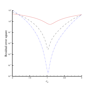
Figure 1: Residual error square versus the convergence control parameter c0subscript๐‘0c_{0} in case of (65) with k2/k1=1subscript๐‘˜2subscript๐‘˜11k_{2}/k_{1}=1.
Table 1: Residual error square of two nonlinear boundary conditions in case of (65) with k2/k1=1subscript๐‘˜2subscript๐‘˜11k_{2}/k_{1}=1
m๐‘šm โ„ฐmฯ•superscriptsubscriptโ„ฐ๐‘šitalic-ฯ•{\cal E}_{m}^{\phi} โ„ฐmฮทsuperscriptsubscriptโ„ฐ๐‘š๐œ‚{\cal E}_{m}^{\eta}
1 1.9 ร—10โˆ’8absentsuperscript108\times 10^{-8} 5.1 ร—10โˆ’4absentsuperscript104\times 10^{-4}
3 3.5 ร—10โˆ’12absentsuperscript1012\times 10^{-12} 1.2 ร—10โˆ’9absentsuperscript109\times 10^{-9}
5 2.0 ร—10โˆ’16absentsuperscript1016\times 10^{-16} 4.3 ร—10โˆ’14absentsuperscript1014\times 10^{-14}
8 2.8 ร—10โˆ’22absentsuperscript1022\times 10^{-22} 3.8ร—10โˆ’20absentsuperscript1020\times 10^{-20}
10 4.7 ร—10โˆ’26absentsuperscript1026\times 10^{-26} 6.4 ร—10โˆ’24absentsuperscript1024\times 10^{-24}

First of all, we consider a special case k2/k1=1subscript๐‘˜2subscript๐‘˜11k_{2}/k_{1}=1. Without loss of generality, we take negative values of A0subscript๐ด0A_{0} and B0subscript๐ต0B_{0} given by (62) and (63), respectively. To choose an optimal value of the convergence-control parameter c0subscript๐‘0c_{0} so that the series solution of ฯ•italic-ฯ•\phi and ฮท๐œ‚\eta converge quickly, we plot the curves of the residual error squares โ„ฐmฯ•superscriptsubscriptโ„ฐ๐‘šitalic-ฯ•{\cal E}_{m}^{\phi} and โ„ฐmฮทsuperscriptsubscriptโ„ฐ๐‘š๐œ‚{\cal E}_{m}^{\eta} versus c0subscript๐‘0c_{0}, as shown in Fig.ย 1. When โ„ฐmฯ•superscriptsubscriptโ„ฐ๐‘šitalic-ฯ•{\cal E}_{m}^{\phi} and โ„ฐmฮทsuperscriptsubscriptโ„ฐ๐‘š๐œ‚{\cal E}_{m}^{\eta} contain the unknown convergence-control parameter c0subscript๐‘0c_{0}, the related integrals are rather time-consuming. To avoid this, a discrete technique suggested by Liao [17] is used. It is found that the residual error square โ„ฐmฯ•superscriptsubscriptโ„ฐ๐‘šitalic-ฯ•{\cal E}_{m}^{\phi} decreases for โˆ’1.8โ‰คc0<01.8subscript๐‘00-1.8\leq c_{0}<0 and the optimal value of c0subscript๐‘0c_{0} is close to -1, as shown in Fig.ย 1. Therefore, we choose c0=โˆ’1subscript๐‘01c_{0}=-1, and the corresponding residual error squares of the two boundary conditions decrease rather quickly to the level 10โˆ’24superscript102410^{-24} at the 10th-order approximation, as listed in Tableย 1. According to the Convergence Theorem mentioned above, the corresponding homotopy-series (38) and (39) are the solution of the problem.

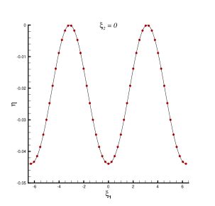
Let a1,0,a0,1subscript๐‘Ž10subscript๐‘Ž01a_{1,0},a_{0,1} and a2,โˆ’1subscript๐‘Ž21a_{2,-1} denote the amplitudes of wave components cosโกฮพ1subscript๐œ‰1\cos\xi_{1}, cosโกฮพ2subscript๐œ‰2\cos\xi_{2} and cosโก(2โ€‹ฮพ1โˆ’ฮพ2)2subscript๐œ‰1subscript๐œ‰2\cos(2\xi_{1}-\xi_{2}), respectively. Obviously, a1,0=a0,1subscript๐‘Ž10subscript๐‘Ž01a_{1,0}=a_{0,1} in case of k1=k2subscript๐‘˜1subscript๐‘˜2k_{1}=k_{2}. As shown in Tableย 2, each wave component converges rather quickly, which agree well (see Tableย 3) with those obtained by the homotopy-Padรฉ method [14, 8], a kind of acceleration technique developed in the frame of the HAM. Besides, the analytic approximations of wave profile at ฮพ2=0subscript๐œ‰20\xi_{2}=0 also converge quickly, as shown in Fig.ย 2. All of these indicate the validity of the analytic approach based on the HAM.

Table 2: Analytic approximations of wave amplitude components in case of (65) with k2/k1=1subscript๐‘˜2subscript๐‘˜11k_{2}/k_{1}=1
Order of appr. a1,0,a0,1subscript๐‘Ž10subscript๐‘Ž01a_{1,0},a_{0,1} a2,โˆ’1subscript๐‘Ž21a_{2,-1}
1 -0.022502 0
2 -0.022846 0.00059739
3 -0.022814 0.00057198
4 -0.022816 0.00057208
6 -0.022816 0.00057226
8 -0.022816 0.00057226
10 -0.022816 0.00057226
Table 3: Analytical approximations of wave amplitude components given by the [m,m]๐‘š๐‘š[m,m] homotopy-Padรฉ method in case of (65) with k2/k1=1subscript๐‘˜2subscript๐‘˜11k_{2}/k_{1}=1
m๐‘šm a1,0,a0,1subscript๐‘Ž10subscript๐‘Ž01a_{1,0},a_{0,1} a2,1subscript๐‘Ž21a_{2,1}
2 -0.022816 0.00057211
3 -0.022816 0.00057226
4 -0.022816 0.00057226
5 -0.022816 0.00057226
\setcaptionwidth

5in Refer to caption

Figure 2: Wave profile at ฮพ2=0subscript๐œ‰20\xi_{2}=0 in case of (65) with k2/k1=1subscript๐‘˜2subscript๐‘˜11k_{2}/k_{1}=1. Symbols: 3rd-order approximation; Solid line: 10th-order approximation.

Similarly, we can get convergent series solutions in case of (65) with different ratio of k2/k1subscript๐‘˜2subscript๐‘˜1k_{2}/k_{1}, as shown in Tableย 4. Note that, as the ratio of k2/k1subscript๐‘˜2subscript๐‘˜1k_{2}/k_{1} decreases, the wave amplitude of the component cosโก(2โ€‹ฮพ1โˆ’ฮพ2)2subscript๐œ‰1subscript๐œ‰2\cos(2\xi_{1}-\xi_{2}) first increases monotonically to the maximum value at k2/k1=0.8925subscript๐‘˜2subscript๐‘˜10.8925k_{2}/k_{1}=0.8925 (the corresponding result is given by the approach described in ยง3.2), and then decreases monotonically. Note that the variation of a1,0subscript๐‘Ž10a_{1,0} and a0,1subscript๐‘Ž01a_{0,1} is not monotonic. It must be emphasized that |a1,0|subscript๐‘Ž10|a_{1,0}| and |a0,1|subscript๐‘Ž01|a_{0,1}| is much larger than |a2,1|subscript๐‘Ž21|a_{2,1}| for all values of k2/k1subscript๐‘˜2subscript๐‘˜1k_{2}/k_{1}, as shown in Tableย  4. We will discuss this interesting phenomena later in details.

Table 4: Wave amplitude components in case of (65) with different values of k2/k1subscript๐‘˜2subscript๐‘˜1k_{2}/k_{1}
k2/k1subscript๐‘˜2subscript๐‘˜1k_{2}/k_{1} a1,0subscript๐‘Ž10a_{1,0} a0,1subscript๐‘Ž01a_{0,1} |a2,1|subscript๐‘Ž21|a_{2,1}|
1.00 -0.0228 -0.0228 0.00057
0.95 -0.0229 -0.0218 0.00084
0.93 -0.0230 -0.0215 0.00116
0.92 -0.0231 -0.0214 0.00150
0.91 -0.0231 -0.0215 0.00219
0.905 -0.0232 -0.0216 0.00290
0.90 -0.023 -0.022 0.00433
0.8925 -0.0205 -0.0232 0.00898
0.88 -0.0235 -0.0179 0.00307
0.86 -0.0221 -0.0189 0.00120
0.85 -0.0226 -0.0187 0.00087
0.83 -0.0229 -0.0182 0.00054
0.80 -0.0232 -0.0172 0.00033
0.70 -0.0239 -0.0121 0.00010

3.2 In case of Nฮป=3subscript๐‘๐œ†3N_{\lambda}=3: resonant waves

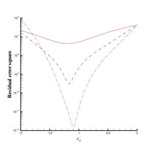
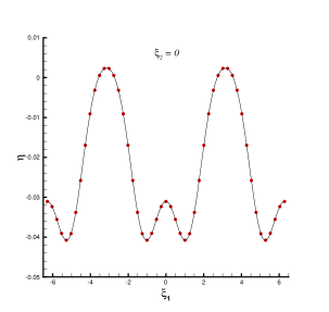
Now, let us further consider the case of (65) with a special ratio k2/k1=0.8925subscript๐‘˜2subscript๐‘˜10.8925k_{2}/k_{1}=0.8925 for two primary traveling waves with wave resonance. It was suggested first by Phillips [1] and then confirmed by Longuet-Higgins [2] that the so-called wave resonance occurs in this case so that the amplitude of wave component cosโก(2โ€‹ฮพ1โˆ’ฮพ2)2subscript๐œ‰1subscript๐œ‰2\cos(2\xi_{1}-\xi_{2}) grows in time, i.e. a2,โˆ’1=ฮฑยฏโ€‹tsubscript๐‘Ž21ยฏ๐›ผ๐‘กa_{2,-1}=\bar{\alpha}\;t , where ฮฑยฏยฏ๐›ผ\bar{\alpha} is a constant.

In this case, the criterion (52) is satisfied, i.e.

gโ€‹|2โ€‹๐ค1โˆ’๐ค2|=(2โ€‹ฯƒยฏ1โˆ’ฯƒยฏ2)2.๐‘”2subscript๐ค1subscript๐ค2superscript2subscriptยฏ๐œŽ1subscriptยฏ๐œŽ22g|2{\bf k}_{1}-{\bf k}_{2}|=(2\bar{\sigma}_{1}-\bar{\sigma}_{2})^{2}.

According to (65), we have

k1=0.703998,k2=0.628319,k3=|2โ€‹๐ค1โˆ’๐ค2|=0.783981.formulae-sequencesubscript๐‘˜10.703998formulae-sequencesubscript๐‘˜20.628319subscript๐‘˜32subscript๐ค1subscript๐ค20.783981k_{1}=0.703998,\;\;k_{2}=0.628319,\;\;k_{3}=|2{\bf k}_{1}-{\bf k}_{2}|=0.783981.

Thus, according to (50), we have an additional zero eigenvalue ฮป2,โˆ’1=0subscript๐œ†210\lambda_{2,-1}=0 with the corresponding eigenfunction

ฮจ2,โˆ’1=e|2โ€‹๐ค1โˆ’๐ค2|โ€‹zโ€‹sinโก(2โ€‹ฮพ1โˆ’ฮพ2).subscriptฮจ21superscript๐‘’2subscript๐ค1subscript๐ค2๐‘ง2subscript๐œ‰1subscript๐œ‰2\Psi_{2,-1}=e^{|2{\bf k}_{1}-{\bf k}_{2}|z}\sin(2\xi_{1}-\xi_{2}).

So, we have now three eigenfunctions ฮจ1,0,ฮจ0,1subscriptฮจ10subscriptฮจ01\Psi_{1,0},\Psi_{0,1} and ฮจ2,โˆ’1subscriptฮจ21\Psi_{2,-1} whose eigenvalues are zero, i.e. ฮป1,0=0subscript๐œ†100\lambda_{1,0}=0, ฮป0,1=0subscript๐œ†010\lambda_{0,1}=0 and ฮป2,โˆ’1=0subscript๐œ†210\lambda_{2,-1}=0. Here, it should be emphasized that the wave resonance condition given by Phillips [1] is mathematically equivalent to that the eigenvalue of nonlinear-interaction wave is zero. Unfortunately, the new zero eigenvalue ฮป2,โˆ’1subscript๐œ†21\lambda_{2,-1} breaks down the approach mentioned in ยง3.1, because the term ฮจ2,โˆ’1/ฮป2,โˆ’1subscriptฮจ21subscript๐œ†21\Psi_{2,-1}/\lambda_{2,-1} in (64) becomes infinite: this is exactly the reason why Phillips [1] and Lenguet-Higgins [2] suggested the existence of the so-called wave-resonance with amplitude growing in time, which, however, is physically impossible from the view-points of wave energy.

Can we avoid such kind of wave-resonance with amplitude growing in time?

Note that, in case of non-resonant waves investigated in ยง3.1, the initial guess (56) is a linear combination of the two eigenfunctions ฮจ1,0subscriptฮจ10\Psi_{1,0} and ฮจ0,1subscriptฮจ01\Psi_{0,1} whose eigenvalues ฮป1,0subscript๐œ†10\lambda_{1,0} and ฮป0,1subscript๐œ†01\lambda_{0,1} are zero. In the current case of wave resonance, the only difference is that we have an additional eigenfunction ฮจ2,โˆ’1subscriptฮจ21\Psi_{2,-1} whose eigenvalue ฮป2,โˆ’1subscript๐œ†21\lambda_{2,-1} is zero, too. As mentioned in many other publications [8, 9, 10, 11, 12, 13, 14, 15, 16], the HAM provides us with great freedom to choose the initial guess. With such kind of freedom, why not use these three eigenfunctions (with zero eigenvalue) to express the initial guess ฯ•0subscriptitalic-ฯ•0\phi_{0}? In other words, we can express the initial guess ฯ•0subscriptitalic-ฯ•0\phi_{0} by all eigenfunctions whose eigenvalues are zero, i.e.

ฯ•0โ€‹(ฮพ1,ฮพ2,z)subscriptitalic-ฯ•0subscript๐œ‰1subscript๐œ‰2๐‘ง\displaystyle\phi_{0}(\xi_{1},\xi_{2},z) =\displaystyle= Aยฏ0โ€‹gk1โ€‹ฮจ1,0+Bยฏ0โ€‹gk2โ€‹ฮจ0,1+Cยฏ0โ€‹gk3โ€‹ฮจ2,โˆ’1,subscriptยฏ๐ด0๐‘”subscript๐‘˜1subscriptฮจ10subscriptยฏ๐ต0๐‘”subscript๐‘˜2subscriptฮจ01subscriptยฏ๐ถ0๐‘”subscript๐‘˜3subscriptฮจ21\displaystyle\bar{A}_{0}\;\sqrt{\frac{g}{k_{1}}}\;\Psi_{1,0}+\bar{B}_{0}\;\sqrt{\frac{g}{k_{2}}}\;\Psi_{0,1}+\bar{C}_{0}\;\sqrt{\frac{g}{k_{3}}}\;\Psi_{2,-1}, (66)

where Aยฏ0,Bยฏ0,Cยฏ0subscriptยฏ๐ด0subscriptยฏ๐ต0subscriptยฏ๐ถ0\bar{A}_{0},\bar{B}_{0},\bar{C}_{0} are unknown constants independent of ฮพ1,ฮพ2subscript๐œ‰1subscript๐œ‰2\xi_{1},\xi_{2} and z๐‘งz. Similarly, substituting the above expression into the deformation equations (40) to (42), we have the same first-order deformation equation (57) with the same boundary condition (59) at bottom for ฯ•1subscriptitalic-ฯ•1\phi_{1}, but a more complicated boundary condition on z=0๐‘ง0z=0, i.e.

โ„’ยฏโ€‹(ฯ•1)ยฏโ„’subscriptitalic-ฯ•1\displaystyle\bar{\cal L}\left(\phi_{1}\right) =\displaystyle= bยฏ11,0โ€‹sinโก(ฮพ1)+bยฏ10,1โ€‹sinโก(ฮพ2)+bยฏ12,0โ€‹sinโก(2โ€‹ฮพ1)+bยฏ13,0โ€‹sinโก(3โ€‹ฮพ1)superscriptsubscriptยฏ๐‘110subscript๐œ‰1superscriptsubscriptยฏ๐‘101subscript๐œ‰2superscriptsubscriptยฏ๐‘1202subscript๐œ‰1superscriptsubscriptยฏ๐‘1303subscript๐œ‰1\displaystyle\bar{b}_{1}^{1,0}\sin(\xi_{1})+\bar{b}_{1}^{0,1}\sin(\xi_{2})+\bar{b}_{1}^{2,0}\sin(2\xi_{1})+\bar{b}_{1}^{3,0}\sin(3\xi_{1}) (67)
+\displaystyle+ bยฏ11,1โ€‹sinโก(ฮพ1+ฮพ2)+dยฏ11,1โ€‹sinโก(ฮพ1โˆ’ฮพ2)superscriptsubscriptยฏ๐‘111subscript๐œ‰1subscript๐œ‰2superscriptsubscriptยฏ๐‘‘111subscript๐œ‰1subscript๐œ‰2\displaystyle\bar{b}_{1}^{1,1}\sin(\xi_{1}+\xi_{2})+\bar{d}_{1}^{1,1}\sin(\xi_{1}-\xi_{2})
+\displaystyle+ bยฏ12,1โ€‹sinโก(2โ€‹ฮพ1+ฮพ2)+dยฏ12,1โ€‹sinโก(2โ€‹ฮพ1โˆ’ฮพ2)superscriptsubscriptยฏ๐‘1212subscript๐œ‰1subscript๐œ‰2superscriptsubscriptยฏ๐‘‘1212subscript๐œ‰1subscript๐œ‰2\displaystyle\bar{b}_{1}^{2,1}\sin(2\xi_{1}+\xi_{2})+\bar{d}_{1}^{2,1}\sin(2\xi_{1}-\xi_{2})
+\displaystyle+ bยฏ11,2โ€‹sinโก(ฮพ1+2โ€‹ฮพ2)+dยฏ11,2โ€‹sinโก(ฮพ1โˆ’2โ€‹ฮพ2)superscriptsubscriptยฏ๐‘112subscript๐œ‰12subscript๐œ‰2superscriptsubscriptยฏ๐‘‘112subscript๐œ‰12subscript๐œ‰2\displaystyle\bar{b}_{1}^{1,2}\sin(\xi_{1}+2\xi_{2})+\bar{d}_{1}^{1,2}\sin(\xi_{1}-2\xi_{2})
+\displaystyle+ dยฏ12,2โ€‹sinโก(2โ€‹ฮพ1โˆ’2โ€‹ฮพ2)+dยฏ12,3โ€‹sinโก(2โ€‹ฮพ1โˆ’3โ€‹ฮพ2)superscriptsubscriptยฏ๐‘‘1222subscript๐œ‰12subscript๐œ‰2superscriptsubscriptยฏ๐‘‘1232subscript๐œ‰13subscript๐œ‰2\displaystyle\bar{d}_{1}^{2,2}\sin(2\xi_{1}-2\xi_{2})+\bar{d}_{1}^{2,3}\sin(2\xi_{1}-3\xi_{2})
+\displaystyle+ dยฏ13,1โ€‹sinโก(3โ€‹ฮพ1โˆ’ฮพ2)+dยฏ13,2โ€‹sinโก(3โ€‹ฮพ1โˆ’2โ€‹ฮพ2)superscriptsubscriptยฏ๐‘‘1313subscript๐œ‰1subscript๐œ‰2superscriptsubscriptยฏ๐‘‘1323subscript๐œ‰12subscript๐œ‰2\displaystyle\bar{d}_{1}^{3,1}\sin(3\xi_{1}-\xi_{2})+\bar{d}_{1}^{3,2}\sin(3\xi_{1}-2\xi_{2})
+\displaystyle+ dยฏ14,1โ€‹sinโก(4โ€‹ฮพ1โˆ’ฮพ2)+dยฏ14,2โ€‹sinโก(4โ€‹ฮพ1โˆ’2โ€‹ฮพ2)+dยฏ14,3โ€‹sinโก(4โ€‹ฮพ1โˆ’3โ€‹ฮพ2)superscriptsubscriptยฏ๐‘‘1414subscript๐œ‰1subscript๐œ‰2superscriptsubscriptยฏ๐‘‘1424subscript๐œ‰12subscript๐œ‰2superscriptsubscriptยฏ๐‘‘1434subscript๐œ‰13subscript๐œ‰2\displaystyle\bar{d}_{1}^{4,1}\sin(4\xi_{1}-\xi_{2})+\bar{d}_{1}^{4,2}\sin(4\xi_{1}-2\xi_{2})+\bar{d}_{1}^{4,3}\sin(4\xi_{1}-3\xi_{2})
+\displaystyle+ dยฏ15,2โ€‹sinโก(5โ€‹ฮพ1โˆ’2โ€‹ฮพ2)+dยฏ16,3โ€‹sinโก(6โ€‹ฮพ1โˆ’3โ€‹ฮพ2),superscriptsubscriptยฏ๐‘‘1525subscript๐œ‰12subscript๐œ‰2superscriptsubscriptยฏ๐‘‘1636subscript๐œ‰13subscript๐œ‰2\displaystyle\bar{d}_{1}^{5,2}\sin(5\xi_{1}-2\xi_{2})+\bar{d}_{1}^{6,3}\sin(6\xi_{1}-3\xi_{2}),

where bยฏ1m,n,dยฏ1m,nsuperscriptsubscriptยฏ๐‘1๐‘š๐‘›superscriptsubscriptยฏ๐‘‘1๐‘š๐‘›\bar{b}_{1}^{m,n},\bar{d}_{1}^{m,n} are constant coefficients, and the linear operator โ„’ยฏยฏโ„’\bar{\cal L} is defined by (45). Note that there exist now three zero eigenvalues, i.e. ฮป1,0=0subscript๐œ†100\lambda_{1,0}=0, ฮป0,1=0subscript๐œ†010\lambda_{0,1}=0 and ฮป2,โˆ’1=0subscript๐œ†210\lambda_{2,-1}=0. Therefore, according to the definition (55) of the inverse operator โ„’ยฏโˆ’1superscriptยฏโ„’1\bar{\cal L}^{-1}, not only the two coefficients bยฏ11,0,bยฏ10,1superscriptsubscriptยฏ๐‘110superscriptsubscriptยฏ๐‘101\bar{b}_{1}^{1,0},\bar{b}_{1}^{0,1} but also the additional coefficient dยฏ12,1superscriptsubscriptยฏ๐‘‘121\bar{d}_{1}^{2,1} must be zero. Enforcing

bยฏ11,0=0,bยฏ10,1=0,dยฏ12,1=0,formulae-sequencesuperscriptsubscriptยฏ๐‘1100formulae-sequencesuperscriptsubscriptยฏ๐‘1010superscriptsubscriptยฏ๐‘‘1210\bar{b}_{1}^{1,0}=0,\;\;\bar{b}_{1}^{0,1}=0,\;\;\bar{d}_{1}^{2,1}=0,

we obtain a set of nonlinear algebraic equations

{12.7576โ€‹Aยฏ02+20.3675โ€‹Bยฏ02+31.6768โ€‹Cยฏ02+25.6718โ€‹Bยฏ0โ€‹Cยฏ0=0.0154469,24.1456โ€‹Aยฏ02+9.6004โ€‹Bยฏ02+30.0398โ€‹Cยฏ02+14.9558โ€‹Aยฏ02โ€‹Cยฏ0/Bยฏ0=0.014593,26.9621โ€‹Aยฏ02+21.6116โ€‹Bยฏ02+16.6956โ€‹Cยฏ02+10.7158โ€‹Aยฏ02โ€‹Bยฏ0/Cยฏ0=0.0163008cases12.7576superscriptsubscriptยฏ๐ด0220.3675superscriptsubscriptยฏ๐ต0231.6768superscriptsubscriptยฏ๐ถ0225.6718subscriptยฏ๐ต0subscriptยฏ๐ถ00.015446924.1456superscriptsubscriptยฏ๐ด029.6004superscriptsubscriptยฏ๐ต0230.0398superscriptsubscriptยฏ๐ถ0214.9558superscriptsubscriptยฏ๐ด02subscriptยฏ๐ถ0subscriptยฏ๐ต00.01459326.9621superscriptsubscriptยฏ๐ด0221.6116superscriptsubscriptยฏ๐ต0216.6956superscriptsubscriptยฏ๐ถ0210.7158superscriptsubscriptยฏ๐ด02subscriptยฏ๐ต0subscriptยฏ๐ถ00.0163008\left\{\begin{array}[]{lcc}12.7576\bar{A}_{0}^{2}+20.3675\bar{B}_{0}^{2}+31.6768\bar{C}_{0}^{2}+25.6718\bar{B}_{0}\bar{C}_{0}&=&0.0154469,\\ 24.1456\bar{A}_{0}^{2}+9.6004\bar{B}_{0}^{2}+30.0398\bar{C}_{0}^{2}+14.9558\bar{A}_{0}^{2}\bar{C}_{0}/\bar{B}_{0}&=&0.014593,\\ 26.9621\bar{A}_{0}^{2}+21.6116\bar{B}_{0}^{2}+16.6956\bar{C}_{0}^{2}+10.7158\bar{A}_{0}^{2}\bar{B}_{0}/\bar{C}_{0}&=&0.0163008\end{array}\right. (68)

for the special case mentioned above. The set of these nonlinear algebraic equations has four complex and twelve real solutions. Because the complex solutions have no physical meanings, we list only its twelve real roots in Tableย 5. It is found that the twelve roots fall into three groups, and different groups give different solutions, as shown later. After solving this set of nonlinear algebraic equations, the initial guess ฯ•0subscriptitalic-ฯ•0\phi_{0} is known and therefore it is straightforward to get ฮท1subscript๐œ‚1\eta_{1} directly by means of (43). More importantly, on the right-hand side of Eq. (67), the terms sinโกฮพ1subscript๐œ‰1\sin\xi_{1}, sinโกฮพ2subscript๐œ‰2\sin\xi_{2} and especially sinโก(2โ€‹ฮพ1โˆ’ฮพ2)2subscript๐œ‰1subscript๐œ‰2\sin(2\xi_{1}-\xi_{2}) disappear now. Then, using the inverse operator (55), it is straightforward to get the common solution of the first-order approximation

ฯ•1subscriptitalic-ฯ•1\displaystyle\phi_{1} =\displaystyle= Aยฏ1โ€‹gk1โ€‹ฮจ1,0+Bยฏ1โ€‹gk2โ€‹ฮจ0,1+Cยฏ1โ€‹gk3โ€‹ฮจ2,โˆ’1subscriptยฏ๐ด1๐‘”subscript๐‘˜1subscriptฮจ10subscriptยฏ๐ต1๐‘”subscript๐‘˜2subscriptฮจ01subscriptยฏ๐ถ1๐‘”subscript๐‘˜3subscriptฮจ21\displaystyle\bar{A}_{1}\sqrt{\frac{g}{k_{1}}}\;\Psi_{1,0}+\bar{B}_{1}\sqrt{\frac{g}{k_{2}}}\;\Psi_{0,1}+\bar{C}_{1}\sqrt{\frac{g}{k_{3}}}\;\Psi_{2,-1} (69)
+\displaystyle+ bยฏ12,0โ€‹(ฮจ2,0ฮป2,0)+bยฏ13,0โ€‹(ฮจ3,0ฮป3,0)+bยฏ11,1โ€‹(ฮจ1,1ฮป1,1)+dยฏ11,1โ€‹(ฮจ1,โˆ’1ฮป1,โˆ’1)superscriptsubscriptยฏ๐‘120subscriptฮจ20subscript๐œ†20superscriptsubscriptยฏ๐‘130subscriptฮจ30subscript๐œ†30superscriptsubscriptยฏ๐‘111subscriptฮจ11subscript๐œ†11superscriptsubscriptยฏ๐‘‘111subscriptฮจ11subscript๐œ†11\displaystyle\bar{b}_{1}^{2,0}\left(\frac{\Psi_{2,0}}{\lambda_{2,0}}\right)+\bar{b}_{1}^{3,0}\left(\frac{\Psi_{3,0}}{\lambda_{3,0}}\right)+\bar{b}_{1}^{1,1}\left(\frac{\Psi_{1,1}}{\lambda_{1,1}}\right)+\bar{d}_{1}^{1,1}\left(\frac{\Psi_{1,-1}}{\lambda_{1,-1}}\right)
+\displaystyle+ bยฏ12,1โ€‹(ฮจ2,1ฮป2,1)+bยฏ11,2โ€‹(ฮจ1,2ฮป1,2)+dยฏ11,2โ€‹(ฮจ1,โˆ’2ฮป1,โˆ’2)+dยฏ12,2โ€‹(ฮจ2,โˆ’2ฮป2,โˆ’2)superscriptsubscriptยฏ๐‘121subscriptฮจ21subscript๐œ†21superscriptsubscriptยฏ๐‘112subscriptฮจ12subscript๐œ†12superscriptsubscriptยฏ๐‘‘112subscriptฮจ12subscript๐œ†12superscriptsubscriptยฏ๐‘‘122subscriptฮจ22subscript๐œ†22\displaystyle\bar{b}_{1}^{2,1}\left(\frac{\Psi_{2,1}}{\lambda_{2,1}}\right)+\bar{b}_{1}^{1,2}\left(\frac{\Psi_{1,2}}{\lambda_{1,2}}\right)+\bar{d}_{1}^{1,2}\left(\frac{\Psi_{1,-2}}{\lambda_{1,-2}}\right)+\bar{d}_{1}^{2,2}\left(\frac{\Psi_{2,-2}}{\lambda_{2,-2}}\right)
+\displaystyle+ dยฏ12,3โ€‹(ฮจ2,โˆ’3ฮป2,โˆ’3)+dยฏ13,1โ€‹(ฮจ3,โˆ’1ฮป3,โˆ’1)+dยฏ13,2โ€‹(ฮจ3,โˆ’2ฮป3,โˆ’2)+dยฏ14,1โ€‹(ฮจ4,โˆ’1ฮป4,โˆ’1)superscriptsubscriptยฏ๐‘‘123subscriptฮจ23subscript๐œ†23superscriptsubscriptยฏ๐‘‘131subscriptฮจ31subscript๐œ†31superscriptsubscriptยฏ๐‘‘132subscriptฮจ32subscript๐œ†32superscriptsubscriptยฏ๐‘‘141subscriptฮจ41subscript๐œ†41\displaystyle\bar{d}_{1}^{2,3}\left(\frac{\Psi_{2,-3}}{\lambda_{2,-3}}\right)+\bar{d}_{1}^{3,1}\left(\frac{\Psi_{3,-1}}{\lambda_{3,-1}}\right)+\bar{d}_{1}^{3,2}\left(\frac{\Psi_{3,-2}}{\lambda_{3,-2}}\right)+\bar{d}_{1}^{4,1}\left(\frac{\Psi_{4,-1}}{\lambda_{4,-1}}\right)
+\displaystyle+ dยฏ14,2โ€‹(ฮจ4,โˆ’2ฮป4,โˆ’2)+dยฏ14,3โ€‹(ฮจ4,โˆ’3ฮป4,โˆ’3)+dยฏ15,2โ€‹(ฮจ5,โˆ’2ฮป5,โˆ’2)+dยฏ16,3โ€‹(ฮจ6,โˆ’3ฮป6,โˆ’3).superscriptsubscriptยฏ๐‘‘142subscriptฮจ42subscript๐œ†42superscriptsubscriptยฏ๐‘‘143subscriptฮจ43subscript๐œ†43superscriptsubscriptยฏ๐‘‘152subscriptฮจ52subscript๐œ†52superscriptsubscriptยฏ๐‘‘163subscriptฮจ63subscript๐œ†63\displaystyle\bar{d}_{1}^{4,2}\left(\frac{\Psi_{4,-2}}{\lambda_{4,-2}}\right)+\bar{d}_{1}^{4,3}\left(\frac{\Psi_{4,-3}}{\lambda_{4,-3}}\right)+\bar{d}_{1}^{5,2}\left(\frac{\Psi_{5,-2}}{\lambda_{5,-2}}\right)+\bar{d}_{1}^{6,3}\left(\frac{\Psi_{6,-3}}{\lambda_{6,-3}}\right).

It should be emphasized that all eigenvalues ฮปm,nsubscript๐œ†๐‘š๐‘›\lambda_{m,n} listed in the above expression are nonzero so that ฯ•1subscriptitalic-ฯ•1\phi_{1} is finite. More importantly, all coefficients in the above expression are independent of the time so that the corresponding wave profile does not grow in time! Note that, like the initial guess ฯ•0subscriptitalic-ฯ•0\phi_{0} defined by (66), the common solution ฯ•1subscriptitalic-ฯ•1\phi_{1} given by (69) has three unknown coefficients Aยฏ1,Bยฏ1subscriptยฏ๐ด1subscriptยฏ๐ต1\bar{A}_{1},\bar{B}_{1} and Cยฏ1subscriptยฏ๐ถ1\bar{C}_{1}, which can be determined similarly by avoiding the โ€œsecularโ€ terms in ฯ•2subscriptitalic-ฯ•2\phi_{2}. So, the above approach has general meanings. Therefore, in a similar way, we can get ฮทmsubscript๐œ‚๐‘š\eta_{m} and ฯ•msubscriptitalic-ฯ•๐‘š\phi_{m} successively, where m=1,2,3๐‘š123m=1,2,3 and so on.

Table 5: Roots of Eq. (68)
Series number
of roots (K๐พK) Aยฏ0subscriptยฏ๐ด0\bar{A}_{0} Bยฏ0subscriptยฏ๐ต0\bar{B}_{0} Cยฏ0subscriptยฏ๐ถ0\bar{C}_{0}
1 (Group-I) -0.0156112 0.0282054 -0.0084973
2 -0.0156112 -0.0282054 0.0084973
3 0.0156112 0.0282054 -0.0084973
4 0.0156112 -0.0282054 0.0084973
5 (Group-II) -0.0155774 -0.0141927 -0.0113800
6 -0.0155774 0.0141927 0.0113800
7 0.0155774 -0.0141927 -0.0113800
8 0.0155774 0.0141927 0.0113800
9 (Group-III) -0.0155626 0.0106109 -0.0226353
10 -0.0155626 -0.0106109 0.0226353
11 0.0155626 0.0106109 -0.0226353
12 0.0155626 -0.0106109 0.0226353

Note that the wave amplitude components a1,0subscript๐‘Ž10a_{1,0} and a0,1subscript๐‘Ž01a_{0,1} in Tableย 4 are negative. To calculate the corresponding wave amplitude components in case of (65) with k2/k1=0.8925subscript๐‘˜2subscript๐‘˜10.8925k_{2}/k_{1}=0.8925, we choose the 2nd root in Group-I, i.e.

Aยฏ0=โˆ’0.0156112,Bยฏ0=โˆ’0.0282054,Cยฏ0=0.00849726.formulae-sequencesubscriptยฏ๐ด00.0156112formulae-sequencesubscriptยฏ๐ต00.0282054subscriptยฏ๐ถ00.00849726\bar{A}_{0}=-0.0156112,\;\;\bar{B}_{0}=-0.0282054,\;\;\bar{C}_{0}=0.00849726.

Similarly, we can choose an optimal value of the so-called convergence-control parameter c0subscript๐‘0c_{0} by plotting the curves of the residual error square โ„ฐmฯ•superscriptsubscriptโ„ฐ๐‘šitalic-ฯ•{\cal E}_{m}^{\phi} versus c0subscript๐‘0c_{0}, as shown in Fig.ย 3, which indicates that the series solution converges in the region โˆ’1.6<c0<01.6subscript๐‘00-1.6<c_{0}<0 and that the optimal value of c0subscript๐‘0c_{0} is close to -1. For simplicity, we take c0=โˆ’1subscript๐‘01c_{0}=-1. The residual error squares โ„ฐmฯ•superscriptsubscriptโ„ฐ๐‘šitalic-ฯ•{\cal E}_{m}^{\phi} and โ„ฐmฮทsuperscriptsubscriptโ„ฐ๐‘š๐œ‚{\cal E}_{m}^{\eta} of the two boundary conditions decrease rapidly to the level 10โˆ’19superscript101910^{-19} (at the 20th-order approximation), as shown in Tableย 6. According to the Convergence Theorem proved in Appendix B, the homotopy-series (38) and (39) satisfy the original governing equation (16) and all boundary conditions (19), (20) and (21). Besides, it is found that the corresponding wave amplitude components a1,0,a0,1subscript๐‘Ž10subscript๐‘Ž01a_{1,0},a_{0,1} and a2,โˆ’1subscript๐‘Ž21a_{2,-1} converge to -0.02051, -0.023212, 0.0089752, respectively, as shown in Tableย 7. To confirm the convergence, we further employ the homotopy-Padรฉ technique [14, 8] to accelerate the convergence and obtain the same convergent wave amplitude components

a1,0=โˆ’0.0205119,a0,1=โˆ’0.0232118,a2,โˆ’1=0.0089752,formulae-sequencesubscript๐‘Ž100.0205119formulae-sequencesubscript๐‘Ž010.0232118subscript๐‘Ž210.0089752a_{1,0}=-0.0205119,\;\;a_{0,1}=-0.0232118,\;\;a_{2,-1}=0.0089752,

as shown in Tableย 9. Furthermore, the corresponding wave profile converges quickly, too, as shown in Figs.ย 5 and 5. Therefore, we indeed get convergent series solution of resonant waves with constant amplitudes even when the resonant condition (52) is exactly satisfied.

Combining the above result with those listed in Tableย 4, we obtain the whole pattern of the dimensionless wave amplitude component k3โ€‹(a2,โˆ’1)subscript๐‘˜3subscript๐‘Ž21k_{3}(a_{2,-1}) versus k2/k1subscript๐‘˜2subscript๐‘˜1k_{2}/k_{1} in case of (65), as shown in Fig.ย 6. It is true that, as the ratio k2/k1subscript๐‘˜2subscript๐‘˜1k_{2}/k_{1} goes to 0.8925, corresponding to the criterion (52) of wave resonance, the dimensionless wave amplitude component k3โ€‹a2,โˆ’1subscript๐‘˜3subscript๐‘Ž21k_{3}\;a_{2,-1} arrives its maximum. Besides, the resonant wave profile in case of k2/k1=0.8925subscript๐‘˜2subscript๐‘˜10.8925k_{2}/k_{1}=0.8925 becomes more complicated, if compared with the non-resonant one in case of k2/k1=1subscript๐‘˜2subscript๐‘˜11k_{2}/k_{1}=1. However, it should be emphasized that the amplitude |a2,โˆ’1|subscript๐‘Ž21|a_{2,-1}| of the wave component cosโก(2โ€‹ฮพ1โˆ’ฮพ2)2subscript๐œ‰1subscript๐œ‰2\cos(2\xi_{1}-\xi_{2}) is a finite constant, even if the resonance condition (52) is satisfied exactly. Besides, it is surprising that, in case of k2/k1=0.8925subscript๐‘˜2subscript๐‘˜10.8925k_{2}/k_{1}=0.8925, the amplitude |a2,โˆ’1|subscript๐‘Ž21|a_{2,-1}| of the resonant wave component is even much smaller than the wave amplitudes |a1,0|subscript๐‘Ž10|a_{1,0}| and |a0,1|subscript๐‘Ž01|a_{0,1}| of the two primary waves!

The above results are obtained by using the 2nd root of Group I in Tableย 5. Similarly, using different roots in Tableย 5, we can search for the corresponding convergent series solutions. It is found that the four different roots of each group in Tableย 5 give the different wave amplitude components a1,0,a0,1subscript๐‘Ž10subscript๐‘Ž01a_{1,0},a_{0,1} and a2,โˆ’1subscript๐‘Ž21a_{2,-1}. But, they have the same absolute values |a1,0|,|a0,1|subscript๐‘Ž10subscript๐‘Ž01|a_{1,0}|,|a_{0,1}| and |a2,โˆ’1|subscript๐‘Ž21|a_{2,-1}|, as listed in Tableย 9. Considering the fact that the wave energy spectrum is determined by the amplitude square of wave components, we regard the four different solutions in each group as the same. Thus, in case of (65) with k2/k1=0.8925subscript๐‘˜2subscript๐‘˜10.8925k_{2}/k_{1}=0.8925, there are three different resonant-wave patterns with different wave energy spectrums. The resonant wave profiles of Group II and III are as shown in Figs.ย 7 and 8. Here, we would like to emphasize that the amplitude |a2,โˆ’1|subscript๐‘Ž21|a_{2,-1}| of the resonant wave is the smallest in Group I, and is the middle in Group II, although it is the largest in Group III. So, the amplitude |a2,โˆ’1|subscript๐‘Ž21|a_{2,-1}| of the resonant wave is not special at all: it is just normal as the wave amplitude components |a1,0|subscript๐‘Ž10|a_{1,0}| and |a0,1|subscript๐‘Ž01|a_{0,1}| of the two primary waves. What we would like to emphasize here is that, for a fully developed wave system, there exist multiple solutions when the resonance condition is exactly satisfied. Besides, the resonant wave amplitude may be much smaller than primary wave amplitudes. These interesting results have not been reported, to the best of our knowledge.

Let ฮ ฮ \Pi denote the sum of amplitude square of all wave components and write

ฮ 0=a1,02+a0,12+a2,โˆ’12.subscriptฮ 0superscriptsubscript๐‘Ž102superscriptsubscript๐‘Ž012superscriptsubscript๐‘Ž212\Pi_{0}=a_{1,0}^{2}+a_{0,1}^{2}+a_{2,-1}^{2}.

It is found that ฮ 0/ฮ =98.82%,98.27%subscriptฮ 0ฮ percent98.82percent98.27\Pi_{0}/\Pi=98.82\%,98.27\% and 99.76%percent99.7699.76\% for Group I, II and III in case of (65) with k2/k1=0.8925subscript๐‘˜2subscript๐‘˜10.8925k_{2}/k_{1}=0.8925 for resonant waves, respectively. This is mainly because amplitudes of other wave components such as a1,โˆ’2subscript๐‘Ž12a_{1,-2} are much smaller, as shown in Tableย 9. Thus, these three wave components nearly contain the whole wave energy. Note that, given two primary traveling waves with wave numbers ๐ค1subscript๐ค1{\bf k}_{1} and ๐ค2subscript๐ค2{\bf k}_{2}, there exist an infinite number of different wave components am,nโ€‹cosโก(mโ€‹ฮพ2+nโ€‹ฮพ2)subscript๐‘Ž๐‘š๐‘›๐‘šsubscript๐œ‰2๐‘›subscript๐œ‰2a_{m,n}\cos(m\xi_{2}+n\xi_{2}) with the wave number mโ€‹๐ค1+nโ€‹๐ค2๐‘šsubscript๐ค1๐‘›subscript๐ค2m{\bf k}_{1}+n{\bf k}_{2}, where m๐‘šm and n๐‘›n are arbitrary integers. Let

๐Š={mโ€‹๐ค1+nโ€‹๐ค2|m,nย are integers}๐Šconditional-set๐‘šsubscript๐ค1๐‘›subscript๐ค2m,nย are integers{\bf K}=\left\{m{\bf k}_{1}+n{\bf k}_{2}|\mbox{$m,n$ are integers}\right\}

denote a set of all these wave numbers. Each wave number in ๐Š๐Š{\bf K} corresponds to an eigenfunction defined by (24) with an eigenvalue defined by (50). Our computations suggest that, for a fully developed wave system with small amplitudes, the main of wave energy focuses on the wave components whose eigenvalues are zero (or close to zero). This provides us an alternative explanation for the so-called wave resonance. According to this explanation, the resonant wave a2,โˆ’1โ€‹cosโก(2โ€‹ฮพ1โˆ’ฮพ2)subscript๐‘Ž212subscript๐œ‰1subscript๐œ‰2a_{2,-1}\cos(2\xi_{1}-\xi_{2}) is as important as the two primary waves a1,0โ€‹cosโกฮพ1subscript๐‘Ž10subscript๐œ‰1a_{1,0}\cos\xi_{1} and a0,1โ€‹cosโกฮพ2subscript๐‘Ž01subscript๐œ‰2a_{0,1}\cos\xi_{2}.

The amplitudes of the resonant waves (related to Group I) in case of ฮฑ1=0,ฮฑ2=ฯ€/36,k2/k1=0.8925formulae-sequencesubscript๐›ผ10formulae-sequencesubscript๐›ผ2๐œ‹36subscript๐‘˜2subscript๐‘˜10.8925\alpha_{1}=0,\alpha_{2}=\pi/36,k_{2}/k_{1}=0.8925 with different ratios of ฯƒ1/gโ€‹k1=ฯƒ2/gโ€‹k2subscript๐œŽ1๐‘”subscript๐‘˜1subscript๐œŽ2๐‘”subscript๐‘˜2\sigma_{1}/\sqrt{gk_{1}}=\sigma_{2}/\sqrt{gk_{2}} are as shown in Tableย 10. The corresponding wave energy distributions are given in Tableย 13. It is found that the two primary waves contain most of the wave energy in this special case. Besides, as the ratio of ฯƒ1/gโ€‹k1=ฯƒ2/gโ€‹k2subscript๐œŽ1๐‘”subscript๐‘˜1subscript๐œŽ2๐‘”subscript๐‘˜2\sigma_{1}/\sqrt{gk_{1}}=\sigma_{2}/\sqrt{gk_{2}} increases, the resonant wave a2,โˆ’1โ€‹cosโก(2โ€‹ฮพ1โˆ’ฮพ2)subscript๐‘Ž212subscript๐œ‰1subscript๐œ‰2a_{2,-1}\cos(2\xi_{1}-\xi_{2}) contains less and less percentage of the whole wave energy. Especially, when ฯƒ1/gโ€‹k1=ฯƒ2/gโ€‹k2=1.0008subscript๐œŽ1๐‘”subscript๐‘˜1subscript๐œŽ2๐‘”subscript๐‘˜21.0008\sigma_{1}/\sqrt{gk_{1}}=\sigma_{2}/\sqrt{gk_{2}}=1.0008, the resonant wave of Group I contains only 2.22% of the whole wave energy. This result is interesting, but a little surprising, because the resonance wave is traditionally supposed to have a large wave amplitude and thus to contain the main of wave energy. We will attempt to explain this phenomena in ยง4. The amplitudes of the resonant waves related to Group II are listed in Tableย 11 and the corresponding wave energy distribution is given in Tableย 14. It is found that the resonant waves of Group II have the comparable wave amplitudes with the comparable percentage of wave energy to one of primary waves. Among three groups, there exists only one group (i.e. Group III) such that the resonant waves have the largest wave amplitude and besides contain the main part of wave energy, as shown in Tableย 12 and Fig.ย 9. Note that, the primary and resonant waves contain the most part of wave energy, especially when all wave amplitude components are very small, as shown in Fig.ย 10. However, as the wave amplitudes increase, the primary and resonant waves contain less and less percentage of wave energy, as shown in Fig.ย 10. This indicates that Phillipsโ€™ wave resonance condition (1) might hold only for small-amplitude traveling waves.

The above results have general meaning, although they are obtained in a special case (65). These results strongly suggest that, for a fully developed system of two traveling waves, all wave amplitudes do not grow linearly in time even if the wave resonance condition is exactly satisfied. This conclusion is also true for arbitrary number of traveling waves, as shown below. Currently, by means of DNS (direct numerical simulation) of the evolution of nonlinear random water waves fields with a continuous spectrum, Annenkov et al [18] investigated the role of exactly resonant, nearly resonant and non-resonant wave interactions, and their results indicate that the amplitudes of wave packets tend to constants. Their results, although obtained for a continuous wave spectrum, support our conclusions mentioned above.

\setcaptionwidth

5in Refer to caption

Figure 3: Residual error square versus the convergence control parameter c0subscript๐‘0c_{0} in case of (65) with k2/k1=0.8925subscript๐‘˜2subscript๐‘˜10.8925k_{2}/k_{1}=0.8925.
Table 6: Residual error square of the two boundary conditions in case of (65) with k2/k1=0.8925subscript๐‘˜2subscript๐‘˜10.8925k_{2}/k_{1}=0.8925
m๐‘šm โ„ฐmฯ•superscriptsubscriptโ„ฐ๐‘šitalic-ฯ•{\cal E}_{m}^{\phi} โ„ฐmฮทsuperscriptsubscriptโ„ฐ๐‘š๐œ‚{\cal E}_{m}^{\eta}
1 4.0 ร—10โˆ’7absentsuperscript107\times 10^{-7} 4.8ร—10โˆ’4absentsuperscript104\times 10^{-4}
3 1.8ร—10โˆ’8absentsuperscript108\times 10^{-8} 1.0ร—10โˆ’6absentsuperscript106\times 10^{-6}
5 2.4 ร—10โˆ’10absentsuperscript1010\times 10^{-10} 1.2ร—10โˆ’8absentsuperscript108\times 10^{-8}
8 1.2 ร—10โˆ’13absentsuperscript1013\times 10^{-13} 1.5ร—10โˆ’11absentsuperscript1011\times 10^{-11}
10 1.3 ร—10โˆ’14absentsuperscript1014\times 10^{-14} 1.2ร—10โˆ’12absentsuperscript1012\times 10^{-12}
15 1.2 ร—10โˆ’17absentsuperscript1017\times 10^{-17} 3.4ร—10โˆ’16absentsuperscript1016\times 10^{-16}
20 1.2 ร—10โˆ’20absentsuperscript1020\times 10^{-20} 1.9ร—10โˆ’19absentsuperscript1019\times 10^{-19}
Table 7: Analytic approximations of wave amplitude components in case of (65) with k2/k1=0.8925subscript๐‘˜2subscript๐‘˜10.8925k_{2}/k_{1}=0.8925
Order of appr. a1,0subscript๐‘Ž10a_{1,0} a0,1subscript๐‘Ž01a_{0,1} a2,โˆ’1subscript๐‘Ž21a_{2,-1}
1 -0.015616 -0.028214 0.0084999
3 -0.020587 -0.023469 0.0094143
5 -0.020533 -0.023231 0.0090083
7 -0.020504 -0.023220 0.0089755
9 -0.020511 -0.023213 0.0089757
11 -0.020512 -0.023212 0.0089753
13 -0.020512 -0.023212 0.0089752
15 -0.020512 -0.023212 0.0089752
18 -0.020512 -0.023212 0.0089752
Table 8: Analytical approximations of wave amplitude components given by the [m,m]๐‘š๐‘š[m,m] homotopy-Padรฉ method in case of (65) with k2/k1=0.8925subscript๐‘˜2subscript๐‘˜10.8925k_{2}/k_{1}=0.8925
m๐‘šm a1,0subscript๐‘Ž10a_{1,0} a0,1subscript๐‘Ž01a_{0,1} a2,โˆ’1subscript๐‘Ž21a_{2,-1}
2 -0.0206010 -0.0232058 0.0089660
3 -0.0204911 -0.0232251 0.0089568
4 -0.0205102 -0.0232172 0.0089780
5 -0.0205122 -0.0232118 0.0089752
6 -0.0205119 -0.0232118 0.0089752
7 -0.0205119 -0.0232118 0.0089752
8 -0.0205119 -0.0232118 0.0089752
9 -0.0205119 -0.0232118 0.0089752
Table 9: Multiple amplitudes of resonant waves in case of (65) with k2/k1=0.8925subscript๐‘˜2subscript๐‘˜10.8925k_{2}/k_{1}=0.8925 given by different roots of Eq. (68) listed in Tableย 5.
|a1,0|subscript๐‘Ž10|a_{1,0}| |a0,1|subscript๐‘Ž01|a_{0,1}| |a2,โˆ’1|subscript๐‘Ž21|a_{2,-1}| |a1,โˆ’2|subscript๐‘Ž12|a_{1,-2}|
Group I 0.02051186921 0.02321179687 0.00897520547 0.00022907754
Group II 0.01475607438 0.01002488089 0.01464333477 0.00096077706
Group III 0.00971236473 0.01032248128 0.02576462018 0.00059968416
Table 10: Amplitudes of resonant waves ( Group I ) in case of ฮฑ1=0,ฮฑ2=ฯ€/36,k2/k1=0.8925formulae-sequencesubscript๐›ผ10formulae-sequencesubscript๐›ผ2๐œ‹36subscript๐‘˜2subscript๐‘˜10.8925\alpha_{1}=0,\alpha_{2}=\pi/36,k_{2}/k_{1}=0.8925 with different ratios of ฯƒ1/gโ€‹k1=ฯƒ2/gโ€‹k2subscript๐œŽ1๐‘”subscript๐‘˜1subscript๐œŽ2๐‘”subscript๐‘˜2\sigma_{1}/\sqrt{gk_{1}}=\sigma_{2}/\sqrt{gk_{2}}.
ฯƒ1/gโ€‹k1,ฯƒ2/gโ€‹k2subscript๐œŽ1๐‘”subscript๐‘˜1subscript๐œŽ2๐‘”subscript๐‘˜2\sigma_{1}/\sqrt{gk_{1}},\sigma_{2}/\sqrt{gk_{2}} |a1,0|subscript๐‘Ž10|a_{1,0}| |a0,1|subscript๐‘Ž01|a_{0,1}| |a2,โˆ’1|subscript๐‘Ž21|a_{2,-1}|
1.0001 0.0117 0.0141 0.0058
1.0002 0.0166 0.0195 0.0078
1.0003 0.0205 0.0232 0.0090
1.0004 0.0238 0.0259 0.0095
1.0005 0.0266 0.0278 0.0096
1.0006 0.0290 0.0291 0.0092
1.0007 0.0312 0.0301 0.0085
1.0008 0.0331 0.0308 0.0076
Table 11: Amplitudes of resonant waves ( Group II ) in case of ฮฑ1=0,ฮฑ2=ฯ€/36,k2/k1=0.8925formulae-sequencesubscript๐›ผ10formulae-sequencesubscript๐›ผ2๐œ‹36subscript๐‘˜2subscript๐‘˜10.8925\alpha_{1}=0,\alpha_{2}=\pi/36,k_{2}/k_{1}=0.8925 with different ratios of ฯƒ1/gโ€‹k1=ฯƒ2/gโ€‹k2subscript๐œŽ1๐‘”subscript๐‘˜1subscript๐œŽ2๐‘”subscript๐‘˜2\sigma_{1}/\sqrt{gk_{1}}=\sigma_{2}/\sqrt{gk_{2}}.
ฯƒ1/gโ€‹k1,ฯƒ2/gโ€‹k2subscript๐œŽ1๐‘”subscript๐‘˜1subscript๐œŽ2๐‘”subscript๐‘˜2\sigma_{1}/\sqrt{gk_{1}},\sigma_{2}/\sqrt{gk_{2}} |a1,0|subscript๐‘Ž10|a_{1,0}| |a0,1|subscript๐‘Ž01|a_{0,1}| |a2,โˆ’1|subscript๐‘Ž21|a_{2,-1}|
1.0001 0.0090 0.0063 0.0084
1.0002 0.0124 0.0085 0.0119
1.0003 0.0148 0.0100 0.0146
1.0004 0.0166 0.0111 0.0169
1.0005 0.0181 0.0120 0.0188
1.0006 0.0194 0.0126 0.0206
1.0007 0.0204 0.0130 0.0222
1.0008 0.0214 0.0134 0.0237
Table 12: Amplitudes of resonant waves ( Group III ) in case of ฮฑ1=0,ฮฑ2=ฯ€/36,k2/k1=0.8925formulae-sequencesubscript๐›ผ10formulae-sequencesubscript๐›ผ2๐œ‹36subscript๐‘˜2subscript๐‘˜10.8925\alpha_{1}=0,\alpha_{2}=\pi/36,k_{2}/k_{1}=0.8925 with different ratios of ฯƒ1/gโ€‹k1=ฯƒ2/gโ€‹k2subscript๐œŽ1๐‘”subscript๐‘˜1subscript๐œŽ2๐‘”subscript๐‘˜2\sigma_{1}/\sqrt{gk_{1}}=\sigma_{2}/\sqrt{gk_{2}}.
ฯƒ1/gโ€‹k1,ฯƒ2/gโ€‹k2subscript๐œŽ1๐‘”subscript๐‘˜1subscript๐œŽ2๐‘”subscript๐‘˜2\sigma_{1}/\sqrt{gk_{1}},\sigma_{2}/\sqrt{gk_{2}} |a1,0|subscript๐‘Ž10|a_{1,0}| |a0,1|subscript๐‘Ž01|a_{0,1}| |a2,โˆ’1|subscript๐‘Ž21|a_{2,-1}|
1.0001 0.0060 0.0060 0.0148
1.0002 0.0082 0.0085 0.0210
1.0003 0.0097 0.0103 0.0258
1.0004 0.0108 0.0118 0.0298
1.0005 0.0116 0.0131 0.0333
1.0006 0.0122 0.0143 0.0365
1.0007 0.0125 0.0153 0.0394
1.0008 0.0127 0.0163 0.0420
Table 13: Wave energy distribution of resonant waves ( Group I ) in case of ฮฑ1=0,ฮฑ2=ฯ€/36,k2/k1=0.8925formulae-sequencesubscript๐›ผ10formulae-sequencesubscript๐›ผ2๐œ‹36subscript๐‘˜2subscript๐‘˜10.8925\alpha_{1}=0,\alpha_{2}=\pi/36,k_{2}/k_{1}=0.8925 with different ratios of ฯƒ1/gโ€‹k1=ฯƒ2/gโ€‹k2subscript๐œŽ1๐‘”subscript๐‘˜1subscript๐œŽ2๐‘”subscript๐‘˜2\sigma_{1}/\sqrt{gk_{1}}=\sigma_{2}/\sqrt{gk_{2}}.
ฯƒ1/gโ€‹k1,ฯƒ2/gโ€‹k2subscript๐œŽ1๐‘”subscript๐‘˜1subscript๐œŽ2๐‘”subscript๐‘˜2\sigma_{1}/\sqrt{gk_{1}},\sigma_{2}/\sqrt{gk_{2}} a1,02/ฮ subscriptsuperscript๐‘Ž210ฮ a^{2}_{1,0}/\Pi a0,12/ฮ subscriptsuperscript๐‘Ž201ฮ a^{2}_{0,1}/\Pi a2,โˆ’12/ฮ subscriptsuperscript๐‘Ž221ฮ a^{2}_{2,-1}/\Pi ฮ 0/ฮ subscriptฮ 0ฮ \Pi_{0}/\Pi
1.0001 36.97% 53.95% 8.99% 99.91%
1.0002 38.40% 52.74% 8.42% 99.56%
1.0003 39.97% 51.19% 7.65% 98.82%
1.0004 41.59% 49.28% 6.70% 97.57%
1.0005 43.10% 47.09% 5.60% 95.78%
1.0006 44.38% 44.75% 4.43% 93.56%
1.0007 45.65% 42.73% 3.58% 91.95%
1.0008 46.23% 39.07% 2.22% 87.52%
Table 14: Wave energy distribution of resonant waves ( Group II ) in case of ฮฑ1=0,ฮฑ2=ฯ€/36,k2/k1=0.8925formulae-sequencesubscript๐›ผ10formulae-sequencesubscript๐›ผ2๐œ‹36subscript๐‘˜2subscript๐‘˜10.8925\alpha_{1}=0,\alpha_{2}=\pi/36,k_{2}/k_{1}=0.8925 with different ratios of ฯƒ1/gโ€‹k1=ฯƒ2/gโ€‹k2subscript๐œŽ1๐‘”subscript๐‘˜1subscript๐œŽ2๐‘”subscript๐‘˜2\sigma_{1}/\sqrt{gk_{1}}=\sigma_{2}/\sqrt{gk_{2}}.
ฯƒ1/gโ€‹k1,ฯƒ2/gโ€‹k2subscript๐œŽ1๐‘”subscript๐‘˜1subscript๐œŽ2๐‘”subscript๐‘˜2\sigma_{1}/\sqrt{gk_{1}},\sigma_{2}/\sqrt{gk_{2}} a1,02/ฮ subscriptsuperscript๐‘Ž210ฮ a^{2}_{1,0}/\Pi a0,12/ฮ subscriptsuperscript๐‘Ž201ฮ a^{2}_{0,1}/\Pi a2,โˆ’12/ฮ subscriptsuperscript๐‘Ž221ฮ a^{2}_{2,-1}/\Pi ฮ 0/ฮ subscriptฮ 0ฮ \Pi_{0}/\Pi
1.0001 42.30% 20.43% 37.07% 99.79%
1.0002 41.26% 19.50% 38.44% 99.20%
1.0003 40.17% 18.54% 39.56% 98.27%
1.0004 39.05% 17.56% 40.44% 97.06%
1.0005 37.93% 16.56% 41.12% 95.61%
1.0006 36.79% 15.54% 41.64% 93.97%
1.0007 35.65% 14.51% 42.02% 92.18%
1.0008 34.49% 13.46% 42.29% 90.24%
Table 15: Wave energy distribution of resonant waves ( Group III ) in case of ฮฑ1=0,ฮฑ2=ฯ€/36,k2/k1=0.8925formulae-sequencesubscript๐›ผ10formulae-sequencesubscript๐›ผ2๐œ‹36subscript๐‘˜2subscript๐‘˜10.8925\alpha_{1}=0,\alpha_{2}=\pi/36,k_{2}/k_{1}=0.8925 with different ratios of ฯƒ1/gโ€‹k1=ฯƒ2/gโ€‹k2subscript๐œŽ1๐‘”subscript๐‘˜1subscript๐œŽ2๐‘”subscript๐‘˜2\sigma_{1}/\sqrt{gk_{1}}=\sigma_{2}/\sqrt{gk_{2}}.
ฯƒ1/gโ€‹k1,ฯƒ2/gโ€‹k2subscript๐œŽ1๐‘”subscript๐‘˜1subscript๐œŽ2๐‘”subscript๐‘˜2\sigma_{1}/\sqrt{gk_{1}},\sigma_{2}/\sqrt{gk_{2}} a1,02/ฮ subscriptsuperscript๐‘Ž210ฮ a^{2}_{1,0}/\Pi a0,12/ฮ subscriptsuperscript๐‘Ž201ฮ a^{2}_{0,1}/\Pi a2,โˆ’12/ฮ subscriptsuperscript๐‘Ž221ฮ a^{2}_{2,-1}/\Pi ฮ 0/ฮ subscriptฮ 0ฮ \Pi_{0}/\Pi
1.0001 12.13% 12.47% 75.37% 99.97%
1.0002 11.53% 12.38% 75.99% 99.90%
1.0003 10.88% 12.29% 76.58% 99.76%
1.0004 10.20% 12.20% 77.15% 99.55%
1.0005 9.47% 12.11% 77.68% 99.26%
1.0006 8.72% 12.01% 78.15% 98.88%
1.0007 7.94% 11.90% 78.53% 98.38%
1.0008 7.15% 11.78% 78.82% 97.75%
\setcaptionwidth

5in Refer to caption

Figure 4: Resonant wave profile at ฮพ2=0subscript๐œ‰20\xi_{2}=0 in case of (65) with k2/k1=0.8925subscript๐‘˜2subscript๐‘˜10.8925k_{2}/k_{1}=0.8925. Symbols: 5th-order approximation; Solid line: 10th-order approximation.
\setcaptionwidth

5in Refer to caption

Figure 5: Resonant wave profile at ฮพ1=0subscript๐œ‰10\xi_{1}=0 in case of (65) with k2/k1=0.8925subscript๐‘˜2subscript๐‘˜10.8925k_{2}/k_{1}=0.8925. Symbols: 5th-order approximation; Solid line: 10th-order approximation.
\setcaptionwidth

5in Refer to caption

Figure 6: The dimensionless wave amplitude component k3โ€‹(a2,โˆ’1)subscript๐‘˜3subscript๐‘Ž21k_{3}(a_{2,-1}) versus k2/k1subscript๐‘˜2subscript๐‘˜1k_{2}/k_{1} in case of (65). Filled circle: result when k2/k1=0.8925subscript๐‘˜2subscript๐‘˜10.8925k_{2}/k_{1}=0.8925; Open circles: results when k2/k1โ‰ 0.8925subscript๐‘˜2subscript๐‘˜10.8925k_{2}/k_{1}\neq 0.8925.
\setcaptionwidth

5in Refer to caption

Figure 7: Resonant wave profile at ฮพ2=0subscript๐œ‰20\xi_{2}=0 in case of (65) with k2/k1=0.8925subscript๐‘˜2subscript๐‘˜10.8925k_{2}/k_{1}=0.8925. Solid line: the 10th-order of approximation of Group II; Dashed line: the 10th-order of approximation of Group III; Symbols: 6th-order approximations.
\setcaptionwidth

5in Refer to caption

Figure 8: Resonant wave profile at ฮพ1=0subscript๐œ‰10\xi_{1}=0 in case of (65) with k2/k1=0.8925subscript๐‘˜2subscript๐‘˜10.8925k_{2}/k_{1}=0.8925. Solid line: the 10th-order of approximation of Group II; Dashed line: the 10th-order of approximation of Group III; Symbols: 6th-order approximations .
\setcaptionwidth

5in Refer to caption

Figure 9: a2,โˆ’12/ฮ subscriptsuperscript๐‘Ž221ฮ a^{2}_{2,-1}/\Pi versus ฯƒ1/gโ€‹k1subscript๐œŽ1๐‘”subscript๐‘˜1\sigma_{1}/\sqrt{gk_{1}} in case of (65) when k2/k1=0.8925subscript๐‘˜2subscript๐‘˜10.8925k_{2}/k_{1}=0.8925 and ฯƒ1/gโ€‹k1=ฯƒ2/gโ€‹k2subscript๐œŽ1๐‘”subscript๐‘˜1subscript๐œŽ2๐‘”subscript๐‘˜2\sigma_{1}/\sqrt{gk_{1}}=\sigma_{2}/\sqrt{gk_{2}} for different group of solutions. Solid line: Group I; Dashed line: Group II; Dash-dotted line: Group III.
\setcaptionwidth

5in Refer to caption

Figure 10: ฮ 0/ฮ subscriptฮ 0ฮ \Pi_{0}/\Pi versus ฯƒ1/gโ€‹k1subscript๐œŽ1๐‘”subscript๐‘˜1\sigma_{1}/\sqrt{gk_{1}} in case of (65) when k2/k1=0.8925subscript๐‘˜2subscript๐‘˜10.8925k_{2}/k_{1}=0.8925 and ฯƒ1/gโ€‹k1=ฯƒ2/gโ€‹k2subscript๐œŽ1๐‘”subscript๐‘˜1subscript๐œŽ2๐‘”subscript๐‘˜2\sigma_{1}/\sqrt{gk_{1}}=\sigma_{2}/\sqrt{gk_{2}} for different group of solutions. Solid line: Group I; Dashed line: Group II; Dash-dotted line: Group III.

4 Resonance condition of arbitrary number of waves

4.1 Resonance condition for small-amplitude waves

In ยง3, we shaw that, for a fully developed system of two primary traveling waves, Phillipsโ€™ resonance condition for small-amplitude waves is exactly equivalent to the zero eigenvalue of the eigenfunction related to the resonant wave. This conclusion has general meanings, and can be easily expanded to give a resonance condition for arbitrary number of travel waves with small amplitude. The key is to give an explicit expression of the eigenvalue in case of arbitrary number of traveling waves.

Let us consider the nonlinear interaction of ฮบ๐œ…\kappa periodic traveling waves with small amplitudes, where 2โ‰คฮบ<+โˆž2๐œ…2\leq\kappa<+\infty is an arbitrary integer. Let ๐คnsubscript๐ค๐‘›{\bf k}_{n} and ฯƒnsubscript๐œŽ๐‘›\sigma_{n} (1โ‰คnโ‰คฮบ1๐‘›๐œ…1\leq n\leq\kappa) denote the given wave number and angular frequency of the n๐‘›nth periodic traveling waves in deep water. Define the variable

ฮพn=๐คmโ‹…๐ซโˆ’ฯƒnโ€‹t,subscript๐œ‰๐‘›โ‹…subscript๐ค๐‘š๐ซsubscript๐œŽ๐‘›๐‘ก\xi_{n}={\bf k}_{m}\cdot{\bf r}-\sigma_{n}\;t,

which has clear physical meanings. Then,

ฯ†โ€‹(x,y,z,t)=ฯ•โ€‹(ฮพ1,ฮพ2,โ‹ฏ,ฮพฮบ,z),ฮถโ€‹(x,y,t)=ฮทโ€‹(ฮพ1,ฮพ2,โ‹ฏ,ฮพฮบ).formulae-sequence๐œ‘๐‘ฅ๐‘ฆ๐‘ง๐‘กitalic-ฯ•subscript๐œ‰1subscript๐œ‰2โ‹ฏsubscript๐œ‰๐œ…๐‘ง๐œ๐‘ฅ๐‘ฆ๐‘ก๐œ‚subscript๐œ‰1subscript๐œ‰2โ‹ฏsubscript๐œ‰๐œ…\varphi(x,y,z,t)=\phi(\xi_{1},\xi_{2},\cdots,\xi_{\kappa},z),\;\;\zeta(x,y,t)=\eta(\xi_{1},\xi_{2},\cdots,\xi_{\kappa}).

Similarly, we have

โˆ‚2ฯ†โˆ‚t2superscript2๐œ‘superscript๐‘ก2\displaystyle\frac{\partial^{2}\varphi}{\partial t^{2}} =\displaystyle= โˆ‘m=1ฮบโˆ‘n=1ฮบฯƒmโ€‹ฯƒnโ€‹โˆ‚2ฯ•โˆ‚ฮพmโ€‹โˆ‚ฮพn,superscriptsubscript๐‘š1๐œ…superscriptsubscript๐‘›1๐œ…subscript๐œŽ๐‘šsubscript๐œŽ๐‘›superscript2italic-ฯ•subscript๐œ‰๐‘šsubscript๐œ‰๐‘›\displaystyle\sum_{m=1}^{\kappa}\sum_{n=1}^{\kappa}\sigma_{m}\sigma_{n}\;\frac{\partial^{2}\phi}{\partial\xi_{m}\partial\xi_{n}}, (70)
โˆ‡ฯ†โˆ‡๐œ‘\displaystyle\nabla\varphi =\displaystyle= (โˆ‘m=1ฮบ๐คmโ€‹โˆ‚ฯ•โˆ‚ฮพm)+๐คโ€‹โˆ‚ฯ•โˆ‚z=๐ฎ=โˆ‡^โ€‹ฯ•,superscriptsubscript๐‘š1๐œ…subscript๐ค๐‘šitalic-ฯ•subscript๐œ‰๐‘š๐คitalic-ฯ•๐‘ง๐ฎ^โˆ‡italic-ฯ•\displaystyle\left(\sum_{m=1}^{\kappa}{\bf k}_{m}\;\frac{\partial\phi}{\partial\xi_{m}}\right)+{\bf k}\frac{\partial\phi}{\partial z}={\bf u}=\hat{\nabla}\phi, (71)
โˆ‡2ฯ†superscriptโˆ‡2๐œ‘\displaystyle\nabla^{2}\varphi =\displaystyle= (โˆ‘m=1ฮบโˆ‘n=1ฮบ๐คmโ‹…๐คnโ€‹โˆ‚2ฯ•โˆ‚ฮพmโ€‹โˆ‚ฮพn)+โˆ‚2ฯ•โˆ‚z2=โˆ‡^2โ€‹ฯ•,superscriptsubscript๐‘š1๐œ…superscriptsubscript๐‘›1๐œ…โ‹…subscript๐ค๐‘šsubscript๐ค๐‘›superscript2italic-ฯ•subscript๐œ‰๐‘šsubscript๐œ‰๐‘›superscript2italic-ฯ•superscript๐‘ง2superscript^โˆ‡2italic-ฯ•\displaystyle\left(\sum_{m=1}^{\kappa}\sum_{n=1}^{\kappa}{\bf k}_{m}\cdot{\bf k}_{n}\;\frac{\partial^{2}\phi}{\partial\xi_{m}\partial\xi_{n}}\right)+\frac{\partial^{2}\phi}{\partial z^{2}}=\hat{\nabla}^{2}\phi, (72)
โˆ‡^โ€‹ฯ•โ‹…โˆ‡^โ€‹ฯ•โ‹…^โˆ‡italic-ฯ•^โˆ‡italic-ฯ•\displaystyle\hat{\nabla}\phi\cdot\hat{\nabla}\phi =\displaystyle= (โˆ‘m=1ฮบโˆ‘n=1ฮบ๐คmโ‹…๐คnโ€‹โˆ‚ฯ•โˆ‚ฮพmโ€‹โˆ‚ฯ•โˆ‚ฮพn)+(โˆ‚ฯ•โˆ‚z)2=๐ฎ2,superscriptsubscript๐‘š1๐œ…superscriptsubscript๐‘›1๐œ…โ‹…subscript๐ค๐‘šsubscript๐ค๐‘›italic-ฯ•subscript๐œ‰๐‘šitalic-ฯ•subscript๐œ‰๐‘›superscriptitalic-ฯ•๐‘ง2superscript๐ฎ2\displaystyle\left(\sum_{m=1}^{\kappa}\sum_{n=1}^{\kappa}{\bf k}_{m}\cdot{\bf k}_{n}\;\frac{\partial\phi}{\partial\xi_{m}}\frac{\partial\phi}{\partial\xi_{n}}\right)+\left(\frac{\partial\phi}{\partial z}\right)^{2}={\bf u}^{2}, (73)
โˆ‡^โ€‹ฯ•โ‹…โˆ‡^โ€‹ฯˆโ‹…^โˆ‡italic-ฯ•^โˆ‡๐œ“\displaystyle\hat{\nabla}\phi\cdot\hat{\nabla}\psi =\displaystyle= (โˆ‘m=1ฮบโˆ‘n=1ฮบ๐คmโ‹…๐คnโ€‹โˆ‚ฯ•โˆ‚ฮพmโ€‹โˆ‚ฯˆโˆ‚ฮพn)+โˆ‚ฯ•โˆ‚zโ€‹โˆ‚ฯˆโˆ‚z.superscriptsubscript๐‘š1๐œ…superscriptsubscript๐‘›1๐œ…โ‹…subscript๐ค๐‘šsubscript๐ค๐‘›italic-ฯ•subscript๐œ‰๐‘š๐œ“subscript๐œ‰๐‘›italic-ฯ•๐‘ง๐œ“๐‘ง\displaystyle\left(\sum_{m=1}^{\kappa}\sum_{n=1}^{\kappa}{\bf k}_{m}\cdot{\bf k}_{n}\;\frac{\partial\phi}{\partial\xi_{m}}\frac{\partial\psi}{\partial\xi_{n}}\right)+\frac{\partial\phi}{\partial z}\frac{\partial\psi}{\partial z}. (74)

Note that

ฮจm1,m2,โ‹ฏ,mฮบ,z=expโก(|โˆ‘n=1ฮบmnโ€‹๐คn|โ€‹z)โ€‹sinโก(โˆ‘n=1ฮบmnโ€‹ฮพn)subscriptฮจsubscript๐‘š1subscript๐‘š2โ‹ฏsubscript๐‘š๐œ…๐‘งsuperscriptsubscript๐‘›1๐œ…subscript๐‘š๐‘›subscript๐ค๐‘›๐‘งsuperscriptsubscript๐‘›1๐œ…subscript๐‘š๐‘›subscript๐œ‰๐‘›\Psi_{m_{1},m_{2},\cdots,m_{\kappa},z}=\exp\left(\left|\sum_{n=1}^{\kappa}m_{n}{\bf k}_{n}\right|z\right)\;\sin\left(\sum_{n=1}^{\kappa}m_{n}\xi_{n}\right) (75)

satisfies the Laplace equation โˆ‡^โ€‹ฯ•=0^โˆ‡italic-ฯ•0\hat{\nabla}\phi=0, i.e.

โˆ‡^2โ€‹ฮจm1,m2,โ‹ฏ,mฮบ=0.superscript^โˆ‡2subscriptฮจsubscript๐‘š1subscript๐‘š2โ‹ฏsubscript๐‘š๐œ…0\hat{\nabla}^{2}\Psi_{m_{1},m_{2},\cdots,m_{\kappa}}=0.

The two nonlinear boundary conditions on the free surface can be written by means of the operators defined above in a similar way. Then, we can construct the zeroth-order deformation equations and the corresponding high-order deformation equations in a similar way as mentioned in ยง3. Although it seems that the governing equations and boundary conditions become much more complicated in form than the original ones by means of these variables, these multiple variables have very clear physical meanings which in fact greatly simplify solving the problem, as described below.

Similarly, we choose such an auxiliary linear operator

โ„’โ€‹ฯ•=(โˆ‘m=1ฮบโˆ‘n=1ฮบฯƒยฏmโ€‹ฯƒยฏnโ€‹โˆ‚2ฯ•โˆ‚ฮพmโ€‹โˆ‚ฮพn)+gโ€‹โˆ‚2ฯ•โˆ‚z2,โ„’italic-ฯ•superscriptsubscript๐‘š1๐œ…superscriptsubscript๐‘›1๐œ…subscriptยฏ๐œŽ๐‘šsubscriptยฏ๐œŽ๐‘›superscript2italic-ฯ•subscript๐œ‰๐‘šsubscript๐œ‰๐‘›๐‘”superscript2italic-ฯ•superscript๐‘ง2{\cal L}\phi=\left(\sum_{m=1}^{\kappa}\sum_{n=1}^{\kappa}\bar{\sigma}_{m}\;\bar{\sigma}_{n}\frac{\partial^{2}\phi}{\partial\xi_{m}\partial\xi_{n}}\right)+g\frac{\partial^{2}\phi}{\partial z^{2}}, (76)

where

ฯƒยฏm=gโ€‹km,km=|๐คm|formulae-sequencesubscriptยฏ๐œŽ๐‘š๐‘”subscript๐‘˜๐‘šsubscript๐‘˜๐‘šsubscript๐ค๐‘š\bar{\sigma}_{m}=\sqrt{g\;k_{m}},\;\;k_{m}=|{\bf k}_{m}|

is based on the linear theory for small-amplitude waves. The above auxiliary linear operator satisfies

โ„’โ€‹(ฮจm1,m2,โ‹ฏ,mฮบ)=ฮปm1,m2,โ‹ฏ,mฮบโ€‹ฮจm1,m2,โ‹ฏ,mฮบ,โ„’subscriptฮจsubscript๐‘š1subscript๐‘š2โ‹ฏsubscript๐‘š๐œ…subscript๐œ†subscript๐‘š1subscript๐‘š2โ‹ฏsubscript๐‘š๐œ…subscriptฮจsubscript๐‘š1subscript๐‘š2โ‹ฏsubscript๐‘š๐œ…{\cal L}\left(\Psi_{m_{1},m_{2},\cdots,m_{\kappa}}\right)=\lambda_{m_{1},m_{2},\cdots,m_{\kappa}}\;\Psi_{m_{1},m_{2},\cdots,m_{\kappa}}, (77)

where

ฮปm1,m2,โ‹ฏ,mฮบ=gโ€‹|โˆ‘n=1ฮบmnโ€‹๐คn|โˆ’(โˆ‘n=1ฮบmnโ€‹ฯƒยฏn)2subscript๐œ†subscript๐‘š1subscript๐‘š2โ‹ฏsubscript๐‘š๐œ…๐‘”superscriptsubscript๐‘›1๐œ…subscript๐‘š๐‘›subscript๐ค๐‘›superscriptsuperscriptsubscript๐‘›1๐œ…subscript๐‘š๐‘›subscriptยฏ๐œŽ๐‘›2\lambda_{m_{1},m_{2},\cdots,m_{\kappa}}=g\left|\sum_{n=1}^{\kappa}m_{n}{\bf k}_{n}\right|-\left(\sum_{n=1}^{\kappa}m_{n}\bar{\sigma}_{n}\right)^{2} (78)

is the eigenvalue and ฮจm1,m2,โ‹ฏ,mฮบsubscriptฮจsubscript๐‘š1subscript๐‘š2โ‹ฏsubscript๐‘š๐œ…\Psi_{m_{1},m_{2},\cdots,m_{\kappa}} defined by (75) is the eigenfunction of the linear operator โ„’โ„’{\cal L} defined by (76). Similarly, the inverse operator of (76) satisfies

โ„’โˆ’1โ€‹(ฮจm1,m2,โ‹ฏ,mฮบ)=ฮจm1,m2,โ‹ฏ,mฮบฮปm1,m2,โ‹ฏ,mฮบ,ฮปm1,m2,โ‹ฏ,mฮบโ‰ 0.formulae-sequencesuperscriptโ„’1subscriptฮจsubscript๐‘š1subscript๐‘š2โ‹ฏsubscript๐‘š๐œ…subscriptฮจsubscript๐‘š1subscript๐‘š2โ‹ฏsubscript๐‘š๐œ…subscript๐œ†subscript๐‘š1subscript๐‘š2โ‹ฏsubscript๐‘š๐œ…subscript๐œ†subscript๐‘š1subscript๐‘š2โ‹ฏsubscript๐‘š๐œ…0{\cal L}^{-1}\left(\Psi_{m_{1},m_{2},\cdots,m_{\kappa}}\right)=\frac{\Psi_{m_{1},m_{2},\cdots,m_{\kappa}}}{\lambda_{m_{1},m_{2},\cdots,m_{\kappa}}},\hskip 28.45274pt\lambda_{m_{1},m_{2},\cdots,m_{\kappa}}\neq 0. (79)

Note that the inverse operator (79) has definition only for non-zero eigenvalue ฮปm1,m2,โ‹ฏ,mฮบsubscript๐œ†subscript๐‘š1subscript๐‘š2โ‹ฏsubscript๐‘š๐œ…\lambda_{m_{1},m_{2},\cdots,m_{\kappa}}. Besides, the eigenvalues of all primary traveling waves are zero, i.e. there exist at least ฮบ๐œ…\kappa zero eigenvalues for ฮบ๐œ…\kappa primary waves. Thus, the so-called wave resonance occurs when there are more than ฮบ๐œ…\kappa zero eigenvalues. So, enforcing ฮปm1,m2,โ‹ฏ,mฮบ=0subscript๐œ†subscript๐‘š1subscript๐‘š2โ‹ฏsubscript๐‘š๐œ…0\lambda_{m_{1},m_{2},\cdots,m_{\kappa}}=0 gives the resonance condition

gโ€‹|โˆ‘n=1ฮบmnโ€‹๐คn|=(โˆ‘n=1ฮบmnโ€‹ฯƒยฏn)2,โˆ‘n=1ฮบmn2>1,formulae-sequence๐‘”superscriptsubscript๐‘›1๐œ…subscript๐‘š๐‘›subscript๐ค๐‘›superscriptsuperscriptsubscript๐‘›1๐œ…subscript๐‘š๐‘›subscriptยฏ๐œŽ๐‘›2superscriptsubscript๐‘›1๐œ…superscriptsubscript๐‘š๐‘›21g\left|\sum_{n=1}^{\kappa}m_{n}{\bf k}_{n}\right|=\left(\sum_{n=1}^{\kappa}m_{n}\bar{\sigma}_{n}\right)^{2},\hskip 28.45274pt\sum_{n=1}^{\kappa}m_{n}^{2}>1, (80)

where ฯƒยฏn=gโ€‹knsubscriptยฏ๐œŽ๐‘›๐‘”subscript๐‘˜๐‘›\bar{\sigma}_{n}=\sqrt{g\;k_{n}} with kn=|๐คn|subscript๐‘˜๐‘›subscript๐ค๐‘›k_{n}=|{\bf k}_{n}| is based on the linear theory for small-amplitude waves. Note that (52) is a special case of the above resonance condition. Besides, the above formula contains the resonance condition given by Phillips [1] and thus is more general.

Assume that, for given ฮบ๐œ…\kappa primary traveling waves, there are Nฮปโ‰ฅฮบsubscript๐‘๐œ†๐œ…N_{\lambda}\geq\kappa eigenfunctions whose eigenvalues are zero. When Nฮป=ฮบsubscript๐‘๐œ†๐œ…N_{\lambda}=\kappa, there is no wave resonance. However, when Nฮป>ฮบsubscript๐‘๐œ†๐œ…N_{\lambda}>\kappa, wave resonance occurs: the wave energy transfers greatly between the resonant wave and primary ones. For simplicity, let ฮจmโˆ—subscriptsuperscriptฮจ๐‘š\Psi^{*}_{m} (1โ‰คmโ‰คNฮป1๐‘šsubscript๐‘๐œ†1\leq m\leq N_{\lambda}) denote the m๐‘šmth eigenfunction with zero eigenvalue. According to (77), it holds

โ„’โ€‹(โˆ‘m=1NฮปAmโ€‹ฮจmโˆ—)=0,Nฮปโ‰ฅฮบformulae-sequenceโ„’superscriptsubscript๐‘š1subscript๐‘๐œ†subscript๐ด๐‘šsuperscriptsubscriptฮจ๐‘š0subscript๐‘๐œ†๐œ…{\cal L}\left(\sum_{m=1}^{N_{\lambda}}A_{m}\;\Psi_{m}^{*}\right)=0,\hskip 28.45274ptN_{\lambda}\geq\kappa (81)

for any constant Amsubscript๐ด๐‘šA_{m}. So, we can always choose such an initial guess that

ฯ•0=โˆ‘m=1NฮปB0,mโ€‹ฮจmโˆ—,subscriptitalic-ฯ•0superscriptsubscript๐‘š1subscript๐‘๐œ†subscript๐ต0๐‘šsuperscriptsubscriptฮจ๐‘š\phi_{0}=\sum_{m=1}^{N_{\lambda}}B_{0,m}\;\Psi_{m}^{*}, (82)

where B0,msubscript๐ต0๐‘šB_{0,m} is unknown. Similarly, the Nฮปsubscript๐‘๐œ†N_{\lambda} unknown constants B0,msubscript๐ต0๐‘šB_{0,m} (1โ‰คmโ‰คNฮป1๐‘šsubscript๐‘๐œ†1\leq m\leq N_{\lambda}) are determined by avoiding the โ€œsecularโ€ terms in ฯ•1subscriptitalic-ฯ•1\phi_{1}. Besides, owing to (81), the common solution of ฯ•1subscriptitalic-ฯ•1\phi_{1} contains Nฮปsubscript๐‘๐œ†N_{\lambda} unknown constants B1,msubscript๐ต1๐‘šB_{1,m} (1โ‰คmโ‰คNฮป1๐‘šsubscript๐‘๐œ†1\leq m\leq N_{\lambda}), which are similarly determined by avoiding the โ€œsecularโ€ terms in ฯ•2subscriptitalic-ฯ•2\phi_{2}. In this way, one can solve the related high-order deformation equations successively, and an optimal value of convergence-control parameter c0subscript๐‘0c_{0} can be chosen so as to ensure the homotopy-series convergent quickly. In theory, the above approach is general, and works for arbitrary number of primary periodic traveling waves with small amplitudes. It provides us a new way to investigate the weakly nonlinear interactions of more than four primary traveling waves with small amplitudes.

4.2 Resonance condition for large wave-amplitude

Note that the general wave resonance condition (80) holds only in case of ฯƒยฏn=gโ€‹knsubscriptยฏ๐œŽ๐‘›๐‘”subscript๐‘˜๐‘›\bar{\sigma}_{n}=\sqrt{g\;k_{n}} with kn=|๐คn|subscript๐‘˜๐‘›subscript๐ค๐‘›k_{n}=|{\bf k}_{n}|, corresponding to small-amplitude gravity waves. What is the resonance condition for arbitrary number of traveling gravity waves with large-amplitude?

\setcaptionwidth

5in Refer to caption

Figure 11: The resonance of a simple pendulum

To answer this question, we should consider the physical meanings of (80). In general, the so-called resonance of a dynamic system occurs when the frequency of an external force (or disturbance) equals to the โ€œnaturalโ€ frequency of the dynamic system. For example, let us consider the resonance of a simple pendulum, as shown in Fig.ย 11, where ๐…=Aโ€‹cosโก(ฯ‰โ€‹t+ฮฑ)๐…๐ด๐œ”๐‘ก๐›ผ{\bf F}=A\;\cos(\omega t+\alpha) is the external force with the frequency ฯ‰๐œ”\omega and the phase difference ฮฑ๐›ผ\alpha. When the maximum angle of oscillation ฮธmโ€‹aโ€‹xsubscript๐œƒ๐‘š๐‘Ž๐‘ฅ\theta_{max} is so small that sinโกฮธโ‰ˆฮธ๐œƒ๐œƒ\sin\theta\approx\theta, the simple pendulum has a natural frequency ฯ‰0โ‰ˆg/lsubscript๐œ”0๐‘”๐‘™\omega_{0}\approx\sqrt{g/l}. So, if the frequency ฯ‰๐œ”\omega of the external force ๐…๐…{\bf F} is equal to the natural frequency ฯ‰0subscript๐œ”0\omega_{0} of the simple pendulum, i.e. ฯ‰=g/l๐œ”๐‘”๐‘™\omega=\sqrt{g/l}, the total energy of the pendulum (and therefore ฮธmโ€‹aโ€‹xsubscript๐œƒ๐‘š๐‘Ž๐‘ฅ\theta_{max}) quickly increases in case of the phase difference ฮฑ=0๐›ผ0\alpha=0 (or decreases in case of ฮฑ=ฯ€๐›ผ๐œ‹\alpha=\pi): the so-called resonance occurs. However, ฯ‰0โ‰ˆg/lsubscript๐œ”0๐‘”๐‘™\omega_{0}\approx\sqrt{g/l} is only valid for small ฮธmโ€‹aโ€‹xsubscript๐œƒ๐‘š๐‘Ž๐‘ฅ\theta_{max}: the natural frequency ฯ‰0subscript๐œ”0\omega_{0} increases as ฮธmโ€‹aโ€‹xsubscript๐œƒ๐‘š๐‘Ž๐‘ฅ\theta_{max} becomes larger. So, as the maximum angle of oscillation ฮธmโ€‹aโ€‹xsubscript๐œƒ๐‘š๐‘Ž๐‘ฅ\theta_{max} becomes so large that the natural frequency ฯ‰0subscript๐œ”0\omega_{0} departs more and more from the frequency ฯ‰=g/l๐œ”๐‘”๐‘™\omega=\sqrt{g/l} of the external force ๐…๐…{\bf F}, then the simple pendulum gains less and less energy from the external force: the maximum angle of oscillation ฮธmโ€‹aโ€‹xsubscript๐œƒ๐‘š๐‘Ž๐‘ฅ\theta_{max} stops increasing when the simple pendulum can not gain energy from ๐…๐…{\bf F} any more in a period of oscillation.

The phenomenon of gravity wave resonance is physically similar to it in essence. For a single traveling wave with the wave number ๐คโ€ฒsuperscript๐คโ€ฒ{\bf k}^{\prime} and the โ€œnaturalโ€ angular frequency ฯƒ0โ€ฒsubscriptsuperscript๐œŽโ€ฒ0\sigma^{\prime}_{0}, the resonance occurs when there exists an โ€œexternalโ€ periodic disturbance with the same angular frequency ฯƒโ€ฒsuperscript๐œŽโ€ฒ\sigma^{\prime}, i.e. ฯƒโ€ฒ=ฯƒ0โ€ฒsuperscript๐œŽโ€ฒsubscriptsuperscript๐œŽโ€ฒ0\sigma^{\prime}=\sigma^{\prime}_{0}. It should be emphasized that this resonance mechanism is physically reasonable even for large wave amplitude.

Let us consider ฮบ๐œ…\kappa primary traveling waves with wave number ๐คnsubscript๐ค๐‘›{\bf k}_{n} and angular frequency ฯƒnsubscript๐œŽ๐‘›\sigma_{n}, where 1โ‰คnโ‰คฮบ1๐‘›๐œ…1\leq n\leq\kappa. Due to nonlinear interaction, there exist a system of an infinite number of wave components

cosโก(โˆ‘n=1ฮบmnโ€‹ฮพn),superscriptsubscript๐‘›1๐œ…subscript๐‘š๐‘›subscript๐œ‰๐‘›\cos\left(\sum_{n=1}^{\kappa}m_{n}\;\xi_{n}\right),

where mnsubscript๐‘š๐‘›m_{n} is an integer that can be negative, zero, or positive. Note that

โˆ‘n=1ฮบmnโ€‹ฮพn=(โˆ‘n=1ฮบmnโ€‹๐คn)โ‹…๐ซโˆ’(โˆ‘n=1ฮบmnโ€‹ฯƒn)โ€‹t.superscriptsubscript๐‘›1๐œ…subscript๐‘š๐‘›subscript๐œ‰๐‘›โ‹…superscriptsubscript๐‘›1๐œ…subscript๐‘š๐‘›subscript๐ค๐‘›๐ซsuperscriptsubscript๐‘›1๐œ…subscript๐‘š๐‘›subscript๐œŽ๐‘›๐‘ก\sum_{n=1}^{\kappa}m_{n}\;\xi_{n}=\left(\sum_{n=1}^{\kappa}m_{n}{\bf k}_{n}\right)\cdot{\bf r}-\left(\sum_{n=1}^{\kappa}m_{n}\;\sigma_{n}\right)t.

So,

๐คโ€ฒ=โˆ‘n=1ฮบmnโ€‹๐คnsuperscript๐คโ€ฒsuperscriptsubscript๐‘›1๐œ…subscript๐‘š๐‘›subscript๐ค๐‘›{\bf k}^{\prime}=\sum_{n=1}^{\kappa}m_{n}\;{\bf k}_{n} (83)

is the wavenumber and

ฯƒโ€ฒ=|โˆ‘n=1ฮบmnโ€‹ฯƒn|superscript๐œŽโ€ฒsuperscriptsubscript๐‘›1๐œ…subscript๐‘š๐‘›subscript๐œŽ๐‘›\sigma^{\prime}=\left|\sum_{n=1}^{\kappa}m_{n}\;\sigma_{n}\right| (84)

is the corresponding angular frequency of the nonlinear-interaction wave. For the sake of simplicity, we call ๐คโ€ฒsuperscript๐คโ€ฒ{\bf k}^{\prime} the nonlinear-interaction wavenumber and ฯƒโ€ฒsuperscript๐œŽโ€ฒ\sigma^{\prime} the nonlinear-interaction angular frequency, respectively, where โˆ‘n=1ฮบmn2>1superscriptsubscript๐‘›1๐œ…superscriptsubscript๐‘š๐‘›21\sum\limits_{n=1}^{\kappa}m_{n}^{2}>1.

For small-amplitude waves, we have ฯƒnโ‰ˆgโ€‹kn=ฯƒยฏnsubscript๐œŽ๐‘›๐‘”subscript๐‘˜๐‘›subscriptยฏ๐œŽ๐‘›\sigma_{n}\approx\sqrt{g\;k_{n}}=\bar{\sigma}_{n}, which leads to

|โˆ‘n=1ฮบmnโ€‹ฯƒยฏn|โ‰ˆ|โˆ‘n=1ฮบmnโ€‹ฯƒn|=ฯƒโ€ฒsuperscriptsubscript๐‘›1๐œ…subscript๐‘š๐‘›subscriptยฏ๐œŽ๐‘›superscriptsubscript๐‘›1๐œ…subscript๐‘š๐‘›subscript๐œŽ๐‘›superscript๐œŽโ€ฒ\left|\sum_{n=1}^{\kappa}m_{n}\;\bar{\sigma}_{n}\right|\approx\left|\sum_{n=1}^{\kappa}m_{n}\;{\sigma}_{n}\right|=\sigma^{\prime} (85)

Substituting the above expression and (83) into (80), we have the resonance condition (for ฮบ๐œ…\kappa small-amplitude primary waves) in the form:

gโ€‹|๐คโ€ฒ|=ฯƒโ€ฒโฃ2,๐‘”superscript๐คโ€ฒsuperscript๐œŽโ€ฒ2g|{\bf k}^{\prime}|=\sigma^{\prime 2},

i.e.

ฯƒโ€ฒ=gโ€‹|๐คโ€ฒ|.superscript๐œŽโ€ฒ๐‘”superscript๐คโ€ฒ\sigma^{\prime}=\sqrt{g|{\bf k}^{\prime}|}. (86)

The above resonance condition clearly reveals the physical relationship between the nonlinear-interaction wavenumber ๐คโ€ฒ=โˆ‘n=1ฮบmnโ€‹๐คnsuperscript๐คโ€ฒsuperscriptsubscript๐‘›1๐œ…subscript๐‘š๐‘›subscript๐ค๐‘›{\bf k}^{\prime}=\sum\limits_{n=1}^{\kappa}m_{n}\;{\bf k}_{n} and the nonlinear-interaction angular frequency ฯƒโ€ฒ=|โˆ‘n=1ฮบmnโ€‹ฯƒn|superscript๐œŽโ€ฒsuperscriptsubscript๐‘›1๐œ…subscript๐‘š๐‘›subscript๐œŽ๐‘›\sigma^{\prime}=\left|\sum\limits_{n=1}^{\kappa}m_{n}\;\sigma_{n}\right|.

Mathematically, the wave resonance condition (86) can be derived in the frame of the HAM. Note that the HAM provides us great freedom to chose the auxiliary linear operator. The auxiliary linear operator โ„’โ„’\cal L defined by (76) contains the term ฯƒยฏi=gโ€‹|๐คi|subscriptยฏ๐œŽ๐‘–๐‘”subscript๐ค๐‘–\bar{\sigma}_{i}=\sqrt{g|{\bf k}_{i}|} which has physical meaning only for small-amplitude waves. So, for large-amplitude waves, we should replace the term ฯƒยฏi=gโ€‹|๐คi|subscriptยฏ๐œŽ๐‘–๐‘”subscript๐ค๐‘–\bar{\sigma}_{i}=\sqrt{g|{\bf k}_{i}|} in (76) by the given angular frequency ฯƒisubscript๐œŽ๐‘–\sigma_{i}. In other words, for primary waves with large-amplitudes, we should choose the auxiliary linear operator

โ„’โ€‹ฯ•=(โˆ‘m=1ฮบโˆ‘n=1ฮบฯƒmโ€‹ฯƒnโ€‹โˆ‚2ฯ•โˆ‚ฮพmโ€‹โˆ‚ฮพn)+gโ€‹โˆ‚2ฯ•โˆ‚z2,โ„’italic-ฯ•superscriptsubscript๐‘š1๐œ…superscriptsubscript๐‘›1๐œ…subscript๐œŽ๐‘šsubscript๐œŽ๐‘›superscript2italic-ฯ•subscript๐œ‰๐‘šsubscript๐œ‰๐‘›๐‘”superscript2italic-ฯ•superscript๐‘ง2{\cal L}\phi=\left(\sum_{m=1}^{\kappa}\sum_{n=1}^{\kappa}\sigma_{m}\;\sigma_{n}\frac{\partial^{2}\phi}{\partial\xi_{m}\partial\xi_{n}}\right)+g\frac{\partial^{2}\phi}{\partial z^{2}}, (87)

where ฯƒisubscript๐œŽ๐‘–\sigma_{i} is the angular frequency of the i๐‘–ith primary wave. In fact, the above linear operator comes from the linear part of the nonlinear boundary condition (5). The eigenvalue of the above linear operator reads

ฮปm1,m2,โ‹ฏ,mฮบ=gโ€‹|โˆ‘n=1ฮบmnโ€‹๐คn|โˆ’(โˆ‘n=1ฮบmnโ€‹ฯƒn)2.subscript๐œ†subscript๐‘š1subscript๐‘š2โ‹ฏsubscript๐‘š๐œ…๐‘”superscriptsubscript๐‘›1๐œ…subscript๐‘š๐‘›subscript๐ค๐‘›superscriptsuperscriptsubscript๐‘›1๐œ…subscript๐‘š๐‘›subscript๐œŽ๐‘›2\lambda_{m_{1},m_{2},\cdots,m_{\kappa}}=g\left|\sum_{n=1}^{\kappa}m_{n}{\bf k}_{n}\right|-\left(\sum_{n=1}^{\kappa}m_{n}\sigma_{n}\right)^{2}. (88)

Enforcing the above formula to be zero, we obtain

|โˆ‘n=1ฮบmnโ€‹ฯƒn|=gโ€‹|โˆ‘n=1ฮบmnโ€‹๐คn|,superscriptsubscript๐‘›1๐œ…subscript๐‘š๐‘›subscript๐œŽ๐‘›๐‘”superscriptsubscript๐‘›1๐œ…subscript๐‘š๐‘›subscript๐ค๐‘›\left|\sum_{n=1}^{\kappa}m_{n}\sigma_{n}\right|=\sqrt{g\left|\sum_{n=1}^{\kappa}m_{n}{\bf k}_{n}\right|}, (89)

which is exactly the wave resonance condition ฯƒโ€ฒ=gโ€‹๐คโ€ฒsuperscript๐œŽโ€ฒ๐‘”superscript๐คโ€ฒ\sigma^{\prime}=\sqrt{g{\bf k}^{\prime}} defined by (86).

Let ฯƒ0โ€ฒsubscriptsuperscript๐œŽโ€ฒ0\sigma^{\prime}_{0} denote the โ€œnaturalโ€ angular frequency of a single traveling wave with the wavenumber ๐คโ€ฒsuperscript๐คโ€ฒ{\bf k}^{\prime} and the wave amplitude aโ€ฒsuperscript๐‘Žโ€ฒa^{\prime}. In case of small wave amplitudes, according to the linear theory, we have the โ€œnaturalโ€ angular frequency ฯƒ0โ€ฒโ‰ˆgโ€‹|๐คโ€ฒ|subscriptsuperscript๐œŽโ€ฒ0๐‘”superscript๐คโ€ฒ\sigma^{\prime}_{0}\approx\sqrt{g\;|{\bf k}^{\prime}|}. Then, the above resonance condition becomes

ฯƒโ€ฒ=ฯƒ0โ€ฒ,superscript๐œŽโ€ฒsubscriptsuperscript๐œŽโ€ฒ0\sigma^{\prime}=\sigma^{\prime}_{0}, (90)

i.e.

|โˆ‘n=1ฮบmnโ€‹ฯƒn|=ฯƒ0โ€ฒ,โˆ‘n=1ฮบmn2>1.formulae-sequencesuperscriptsubscript๐‘›1๐œ…subscript๐‘š๐‘›subscript๐œŽ๐‘›subscriptsuperscript๐œŽโ€ฒ0superscriptsubscript๐‘›1๐œ…superscriptsubscript๐‘š๐‘›21\left|\sum_{n=1}^{\kappa}m_{n}\;{\sigma}_{n}\right|=\sigma^{\prime}_{0},\;\;\hskip 28.45274pt\sum_{n=1}^{\kappa}m_{n}^{2}>1. (91)

Physically speaking, the wave resonance occurs when the nonlinear-interaction angular frequency ฯƒโ€ฒ=|โˆ‘n=1ฮบmnโ€‹ฯƒn|superscript๐œŽโ€ฒsuperscriptsubscript๐‘›1๐œ…subscript๐‘š๐‘›subscript๐œŽ๐‘›\sigma^{\prime}=\left|\sum\limits_{n=1}^{\kappa}m_{n}\;{\sigma}_{n}\right| of the corresponding nonlinear-interaction wave with wavenumber ๐คโ€ฒ=โˆ‘n=1ฮบmnโ€‹๐คnsuperscript๐คโ€ฒsuperscriptsubscript๐‘›1๐œ…subscript๐‘š๐‘›subscript๐ค๐‘›{\bf k}^{\prime}=\sum\limits_{n=1}^{\kappa}m_{n}\;{\bf k}_{n} equals to its โ€œnaturalโ€ angular frequency ฯƒ0โ€ฒsubscriptsuperscript๐œŽโ€ฒ0\sigma^{\prime}_{0}. Note that, different from the nonlinear-interaction angular frequency ฯƒโ€ฒsuperscript๐œŽโ€ฒ\sigma^{\prime} that is a kind of sum of angular frequencies of primary waves, the โ€œnaturalโ€ angular frequency ฯƒ0โ€ฒsubscriptsuperscript๐œŽโ€ฒ0\sigma^{\prime}_{0} of the corresponding wave number ๐คโ€ฒsuperscript๐คโ€ฒ{\bf k}^{\prime} depends only upon the wavenumber ๐คโ€ฒsuperscript๐คโ€ฒ{\bf k}^{\prime} and its amplitude aโ€ฒsuperscript๐‘Žโ€ฒa^{\prime}, but has nothing to do with the angular frequencies of primary waves. Thus, in general, the nonlinear-interaction angular frequency ฯƒโ€ฒsuperscript๐œŽโ€ฒ\sigma^{\prime} is not equal to the โ€œnaturalโ€ angular frequency ฯƒ0โ€ฒsubscriptsuperscript๐œŽโ€ฒ0\sigma^{\prime}_{0} of the nonlinear-interaction wave with wavenumber ๐คโ€ฒsuperscript๐คโ€ฒ{\bf k}^{\prime}. So, the wave resonance condition is indeed rather special. This physical explanation agrees well with the traditional resonance theory. So, (90) and (91) reveal the physical essence of the gravity wave resonance.

Although (91) is derived from the resonance condition (80) for small wave amplitudes, this physical mechanism of gravity wave resonance has general meanings and holds for large wave amplitudes even if ฯƒnโ‰ˆgโ€‹knsubscript๐œŽ๐‘›๐‘”subscript๐‘˜๐‘›\sigma_{n}\approx\sqrt{g\;k_{n}} is not a good approximation. So, (91) is also the wave resonance condition for arbitrary number of primary waves with large amplitudes. It should be emphasized that the wave resonance condition (91) logically contains the resonance condition (80) for arbitrary number of small-amplitude waves and Phillipsโ€™ resonance condition (1) for four small-amplitude waves. Thus, it is rather general.

When the wave resonance condition (91) is satisfied and the wave energy transfers from the primary waves to a resonant one, the amplitudes of primary waves decreases and the amplitude of the resonant wave increases. Therefore, the angular frequencies ฯƒnsubscript๐œŽ๐‘›\sigma_{n} of each primary waves decrease but the โ€œnaturalโ€ angular frequency of the resonant wave increases so that the resonance condition (91) does not hold any more. As a result, the โ€œnaturalโ€ frequency ฯƒ0โ€ฒsubscriptsuperscript๐œŽโ€ฒ0\sigma^{\prime}_{0} departs more and more from the nonlinear-interaction frequency ฯƒโ€ฒsuperscript๐œŽโ€ฒ\sigma^{\prime}, and the nonlinear-interaction wave gains less and less energy from the primary waves, until the whole wave system is in equilibrium. This explains why a resonant gravity wave has finite value of amplitude. As mentioned above, a resonant simple pendulum acted by an external force with the phase difference ฯ€๐œ‹\pi, as shown in Fig.11, loses its energy so that the maximum angel of oscillation ฮธmโ€‹aโ€‹xsubscript๐œƒ๐‘š๐‘Ž๐‘ฅ\theta_{max} decreases. Similarly, when the wave resonance condition (91) is satisfied, it is also possible that the wave energy transfers from the resonant wave to primary ones so that the amplitude of resonant wave decreases and the amplitudes of primary waves increase: this explains why the amplitude of a resonant wave may be much smaller than those of primary ones, as shown in Tableย 13.

5 Concluding remark and discussions

The main findings and concluding remarks are outlined below.

First of all, based on a analytic technique for strongly nonlinear problems, namely the homotopy analysis method (HAM), a multiple-variable technique is proposed and applied to give convergent series solution of a fully developed system of arbitrary number of primary periodic traveling waves. Different from perturbation techniques used by Phillips [1] and Longuet-Higgins [2], this multiple-variable technique does not depend upon any small physical parameters, and besides provides a convenient way to ensure the fast convergence of solution series. By means of this multiple-variable technique, the time t๐‘กt does not explicitly appear for a fully developed wave system: this not only greatly simplifies solving the problem mathematically, but also contributes a lot to revealing the physical meanings clearly (some users of the HAM solved nonlinear wave-type PDEs by simply expanding the solution in Taylor series with respect to the time t๐‘กt. Unfortunately, this often leads to very complicated solution expressions with rather little physical meanings). Thus, the homotopy multiple-variable method has general meanings and can be widely applied to different types of nonlinear problems in science and engineering. For example, although this method is used here for fully developed gravity waves, it can be applied to study the evolution of nonlinear waves far from equilibrium (such as the famous natural phenomena about freak wave [19, 20, 21]), as long as we introduce a โ€œslowโ€ time-scale ฯ„=t/(1+t)๐œ๐‘ก1๐‘ก\tau=t/(1+t) as an additional variable to describe the time-dependent variation of the wave amplitude and angular frequency.

Secondly, by means of the homotopy multiple-variable method, we illustrated that the amplitudes of all wave components of a fully developed wave system are finite constants, even if the resonance condition is exactly satisfied. Besides, we revealed, maybe for the first time, that a fully developed resonant wave system may have multiple solutions. Especially, it is found that the amplitude of resonant waves might be much smaller than that of primary waves, and that a resonant wave may contain only the few of the whole wave energy. These results differ from some of our traditional thoughts, but strongly suggest that, due to nonlinear interaction, the evolution of a multiple-wave system might be rather complicated. At the end of ยง4, some physical explanations for these results are given.

Third, by means of the homotopy multiple-variable method, we derived two general wave resonance conditions (80) and (91) for arbitrary number of primary periodic traveling waves: the former holds for small-amplitude waves, but the latter works even for large-amplitude waves. These two resonance conditions logically contain Phillipsโ€™ resonance condition (1) for four small-amplitude waves, and thus are more general. Especially, the wave resonance condition (91) opens a new way to study the strongly nonlinear interactions of more than four primary traveling waves with large amplitudes.

Mathematically, our computations suggest that, for a fully developed wave system with small amplitudes, the main wave energy distribute in the wave components whose eigenvalues to the linear operator (76) or (87) are zero (or close to zero). Physically speaking, the primary and resonant waves contain the main of the wave energy. However, as the wave amplitudes increases so that the nonlinearity becomes stronger, the primary and resonant waves as a whole contain less and less percentage of wave energy, as shown in Fig.ย 10.

There are some open questions. The resonance condition (91) for arbitrary number of traveling waves with large amplitudes is given from the physical view-points of resonance. Although this resonance condition explains very well why the amplitude of a resonant wave is finite and why it can be much smaller than those of primary ones, it should be verified by experiments or other analytical/numerical approaches. Besides, it is worthwhile studying the evolution of a system of multiple traveling waves far from equilibrium.

Finally, it should be pointed out once again that the homotopy multiple-variable method proposed in this article is more general than the famous multiple-scales techniques in perturbation theory. By means of the perturbation multiple-scale technique, one often rewrites a unknown function fโ€‹(t)๐‘“๐‘กf(t) in the form Fโ€‹(T0,T1,T2)๐นsubscript๐‘‡0subscript๐‘‡1subscript๐‘‡2F(T_{0},T_{1},T_{2}), where

T0=t,T1=ฯตโ€‹t,T2=ฯต2โ€‹tformulae-sequencesubscript๐‘‡0๐‘กformulae-sequencesubscript๐‘‡1italic-ฯต๐‘กsubscript๐‘‡2superscriptitalic-ฯต2๐‘กT_{0}=t,\;\;T_{1}=\epsilon\;t,\;\;T_{2}=\epsilon^{2}\;t

denote different timescales with the small physical parameter ฯตitalic-ฯต\epsilon. By means of this traditional multiple-scale technique, a nonlinear problem is often transformed into a sequence of linear perturbed problems via the small physical parameter ฯตitalic-ฯต\epsilon. Using the homotopy multiple-variable method, we can also rewrite fโ€‹(t)๐‘“๐‘กf(t) by Fห‡โ€‹(ฮพ0,ฮพ1,ฮพ2)ห‡๐นsubscript๐œ‰0subscript๐œ‰1subscript๐œ‰2\check{F}(\xi_{0},\xi_{1},\xi_{2}) with the definition

ฮพn=ฯตnโ€‹t.subscript๐œ‰๐‘›superscriptitalic-ฯต๐‘›๐‘ก\xi_{n}=\epsilon^{n}\;t.

However, different from the multiple-scale perturbation techniques, we now do not need any small physical parameters to transform the original nonlinear problem into a sequence of linear sub-problems. Furthermore, it is easy to get high-order approximation by our approach, as illustrated in this article. Especially, if the multiple-variables are properly defined with clear physical meanings, this method is helpful to get results with important physical meanings. This work illustrates that the homotopy multiple-variable method can overcome the restrictions of traditional analytic methods and besides it belongs to the times of computer. It seems that the homotopy multiple-variable technique can be applied widely to solve different types of strongly nonlinear problems in science and engineering.

Acknowledgements Thanks to Professor Roger Grimshaw (Loughborough University, UK) for some discussions about gravity wave resonance via emails, and to Dr. Zhiliang Lin (Shanghai Jiaotong University) for his assistance in plotting the figure for the simple pendulum. This work is supported by National Natural Science Foundation of China (Approve No. 10572095) and State Key Laboratory of Ocean Engineering (Approve No. GKZD010002).

References

  • [1] Phillips, O.M. On the dynamics of unsteady gravity waves of finite amplitude. Part 1. The elementary interactions. J. Fluid Mech., 9:193โ€“217, 1960.
  • [2] Longuet-Higgins, M.S. Resonant interactions between two trains of gravity waves. J. Fluid Mech., 12:321โ€“332, 1962.
  • [3] Longuet-Higgins, M.S. and Smith, N.D. An experiment on third order resonant wave interactions. J. Fluid Mech., 25:417โ€“435, 1966.
  • [4] McGoldrick, L.F., Phillips, O.M., Huang, N. and Hodgson, T. Measurements on resonant wave interactions. J. Fluid Mech., 25:437โ€“456, 1966.
  • [5] Benney, D.T. Non-linear gravity wave interactions. J. Fluid Mech., 14:577โ€“584, 1962.
  • [6] Bretherton, F.P. Resonant interactions between waves: the case of discrete oscillations. J. Fluid Mech., 20:457โ€“479, 1964.
  • [7] Phillips, O.M. Wave interactions- the evolution of an idea. J. Fluid Mech., 106:215โ€“227, 1981.
  • [8] Liao, S.J. Beyond Perturbation: Introduction to the Homotopy Analysis Method. Chapman & Hall/ CRC Press, Boca Raton, 2003.
  • [9] Liao, S.J. An explicit, totally analytic approximation of Blasius viscous flow problems. Int. J. of Non-Linear Mech., 34(4):759โ€“778, 1999.
  • [10] Liao, S.J. A uniformly valid analytic solution of 2D viscous flow past a semi-infinite flat plate. J. Fluid Mech., 385:101โ€“128, 1999.
  • [11] Liao, S.J. and Campo, A. Analytic solutions of the temperature distribution in Blasius viscous flow problems. J. Fluid Mech., 453:411โ€“425, 2002.
  • [12] Liao, S.J. On the analytic solution of magnetohydrodynamic flows of non-Newtonian fluids over a stretching sheet. J. Fluid Mech., 488:189โ€“212, 2003.
  • [13] Liao, S.J. Series solutions of unsteady boundary-layer flows over a stretching flat plate. Studies in Applied Mathematics, 117(3):2529โ€“2539, 2006.
  • [14] Liao, S.J. and Tan, Y. A general approach to obtain series solutions of nonlinear differential equations. Studies in Applied Mathematics, 119:297โ€“355, 2007.
  • [15] Xu, H., Lin, Z.L., Liao, S.J., Wu, J.Z.and Majdalani, J. Homotopy-based solutions of the Navier-Stokes equations for a porous channel with orthogonally moving walls. Physics of Fluids, 22, 2010. online.
  • [16] Li, Y.J., Nohara, B.T. and Liao, S.J. Series solutions of coupled Van der Pol equation by means of homotopy analysis method. J. Mathematical Physics. online.
  • [17] Liao, S.J. An optimal homotopy-analysis approach for strongly nonlinear differential equations. Communications in Nonlinear Science and Numerical Simulation, 15:2003โ€“2016, 2010.
  • [18] Annenkov S.Y. and Shrira, V.I. Role of non-resonant interactions in the evolution of nonlinear random water wave fields. J. Fluid Mech., 561:181โ€“207, 2006.
  • [19] Kharif, C. and Pelinovsky, E. Physical mechanisms of the rogue wave phenomenon. Eur. J. Mech. B - Fluids, 22:603โ€“634, 2003.
  • [20] Gibbs, R.H. and Taylor, P.H. Formation of walls of water in โ€˜fullyโ€™ nonlinear simulations. Applied Ocean Research, 27:142โ€“257, 2005.
  • [21] Adcock, T.A.A. and Taylor, P.H. Focusing of unidirectional wave groups on deep water: an approximate nonlinear Schrรถdinger equation-based model. Proceedings of the Royal Society:A, 465:3083โ€“3102, 2009.

Appendix A
The detailed derivation of (42) and (43)

Write

(โˆ‘i=1+โˆžฮทiโ€‹qi)m=โˆ‘n=m+โˆžฮผm,nโ€‹qn,superscriptsuperscriptsubscript๐‘–1subscript๐œ‚๐‘–superscript๐‘ž๐‘–๐‘šsuperscriptsubscript๐‘›๐‘šsubscript๐œ‡๐‘š๐‘›superscript๐‘ž๐‘›\left(\sum_{i=1}^{+\infty}\eta_{i}\;q^{i}\right)^{m}=\sum_{n=m}^{+\infty}\mu_{m,n}\;q^{n}, (92)

with the definition

ฮผ1,nโ€‹(ฮพ1,ฮพ2)=ฮทnโ€‹(ฮพ1,ฮพ2),nโ‰ฅ1.formulae-sequencesubscript๐œ‡1๐‘›subscript๐œ‰1subscript๐œ‰2subscript๐œ‚๐‘›subscript๐œ‰1subscript๐œ‰2๐‘›1\mu_{1,n}(\xi_{1},\xi_{2})=\eta_{n}(\xi_{1},\xi_{2}),\;\;n\geq 1. (93)

Then,

(โˆ‘i=1+โˆžฮทiโ€‹qi)m+1=(โˆ‘n=m+โˆžฮผm,nโ€‹qn)โ€‹(โˆ‘i=1+โˆžฮทiโ€‹qi)superscriptsuperscriptsubscript๐‘–1subscript๐œ‚๐‘–superscript๐‘ž๐‘–๐‘š1superscriptsubscript๐‘›๐‘šsubscript๐œ‡๐‘š๐‘›superscript๐‘ž๐‘›superscriptsubscript๐‘–1subscript๐œ‚๐‘–superscript๐‘ž๐‘–\displaystyle\left(\sum_{i=1}^{+\infty}\eta_{i}\;q^{i}\right)^{m+1}=\left(\sum_{n=m}^{+\infty}\mu_{m,n}\;q^{n}\right)\left(\sum_{i=1}^{+\infty}\eta_{i}\;q^{i}\right) (94)
=\displaystyle= โˆ‘s=m+1+โˆžqsโ€‹(โˆ‘n=msโˆ’1ฮผm,nโ€‹ฮทsโˆ’n)=โˆ‘n=m+1+โˆžqnโ€‹(โˆ‘i=mnโˆ’1ฮผm,iโ€‹ฮทnโˆ’i)superscriptsubscript๐‘ ๐‘š1superscript๐‘ž๐‘ superscriptsubscript๐‘›๐‘š๐‘ 1subscript๐œ‡๐‘š๐‘›subscript๐œ‚๐‘ ๐‘›superscriptsubscript๐‘›๐‘š1superscript๐‘ž๐‘›superscriptsubscript๐‘–๐‘š๐‘›1subscript๐œ‡๐‘š๐‘–subscript๐œ‚๐‘›๐‘–\displaystyle\sum_{s=m+1}^{+\infty}q^{s}\left(\sum_{n=m}^{s-1}\mu_{m,n}\;\eta_{s-n}\right)=\sum_{n=m+1}^{+\infty}q^{n}\left(\sum_{i=m}^{n-1}\mu_{m,i}\;\eta_{n-i}\right)
=\displaystyle= โˆ‘j=m+1+โˆžฮผm+1,nโ€‹qn,superscriptsubscript๐‘—๐‘š1subscript๐œ‡๐‘š1๐‘›superscript๐‘ž๐‘›\displaystyle\sum_{j=m+1}^{+\infty}\mu_{m+1,n}\;q^{n},

which gives

ฮผm+1,nโ€‹(ฮพ1,ฮพ2)=โˆ‘i=mnโˆ’1ฮผm,iโ€‹(ฮพ1,ฮพ2)โ€‹ฮทnโˆ’iโ€‹(ฮพ1,ฮพ2),mโ‰ฅ1,nโ‰ฅm+1,formulae-sequencesubscript๐œ‡๐‘š1๐‘›subscript๐œ‰1subscript๐œ‰2superscriptsubscript๐‘–๐‘š๐‘›1subscript๐œ‡๐‘š๐‘–subscript๐œ‰1subscript๐œ‰2subscript๐œ‚๐‘›๐‘–subscript๐œ‰1subscript๐œ‰2formulae-sequence๐‘š1๐‘›๐‘š1\mu_{m+1,n}(\xi_{1},\xi_{2})=\sum_{i=m}^{n-1}\mu_{m,i}(\xi_{1},\xi_{2})\;\eta_{n-i}(\xi_{1},\xi_{2}),\;\;\;m\geq 1,\;n\geq m+1,

i.e.

ฮผm,nโ€‹(ฮพ1,ฮพ2)=โˆ‘i=mโˆ’1nโˆ’1ฮผmโˆ’1,iโ€‹(ฮพ1,ฮพ2)โ€‹ฮทnโˆ’iโ€‹(ฮพ1,ฮพ2),mโ‰ฅ2,nโ‰ฅm.formulae-sequencesubscript๐œ‡๐‘š๐‘›subscript๐œ‰1subscript๐œ‰2superscriptsubscript๐‘–๐‘š1๐‘›1subscript๐œ‡๐‘š1๐‘–subscript๐œ‰1subscript๐œ‰2subscript๐œ‚๐‘›๐‘–subscript๐œ‰1subscript๐œ‰2formulae-sequence๐‘š2๐‘›๐‘š\mu_{m,n}(\xi_{1},\xi_{2})=\sum_{i=m-1}^{n-1}\mu_{m-1,i}(\xi_{1},\xi_{2})\;\eta_{n-i}(\xi_{1},\xi_{2}),\;\;\;m\geq 2,\;n\geq m. (95)

Thus, by means of (93) and (95), one can easily get ฮผm,nsubscript๐œ‡๐‘š๐‘›\mu_{m,n} even for large m๐‘šm and n๐‘›n.

Define

ฯˆi,jn,mโ€‹(ฮพ1,ฮพ2)=โˆ‚i+jโˆ‚ฮพ1iโ€‹โˆ‚ฮพ2jโ€‹(1m!โ€‹โˆ‚mฯ•nโˆ‚zm|z=0).superscriptsubscript๐œ“๐‘–๐‘—๐‘›๐‘šsubscript๐œ‰1subscript๐œ‰2superscript๐‘–๐‘—superscriptsubscript๐œ‰1๐‘–superscriptsubscript๐œ‰2๐‘—evaluated-at1๐‘šsuperscript๐‘šsubscriptitalic-ฯ•๐‘›superscript๐‘ง๐‘š๐‘ง0\psi_{i,j}^{n,m}(\xi_{1},\xi_{2})=\frac{\partial^{i+j}}{\partial\xi_{1}^{i}\partial\xi_{2}^{j}}\left(\frac{1}{m!}\;\left.\frac{\partial^{m}\phi_{n}}{\partial z^{m}}\right|_{z=0}\right).

By Taylor series, we have for any z๐‘งz that

ฯ•nโ€‹(ฮพ1,ฮพ2,z)=โˆ‘m=0+โˆž(1m!โ€‹โˆ‚mฯ•nโˆ‚zm|z=0)โ€‹zm=โˆ‘m=0+โˆžฯˆ0,0n,mโ€‹zmsubscriptitalic-ฯ•๐‘›subscript๐œ‰1subscript๐œ‰2๐‘งsuperscriptsubscript๐‘š0evaluated-at1๐‘šsuperscript๐‘šsubscriptitalic-ฯ•๐‘›superscript๐‘ง๐‘š๐‘ง0superscript๐‘ง๐‘šsuperscriptsubscript๐‘š0superscriptsubscript๐œ“00๐‘›๐‘šsuperscript๐‘ง๐‘š\phi_{n}(\xi_{1},\xi_{2},z)=\sum_{m=0}^{+\infty}\left(\left.\frac{1}{m!}\;\frac{\partial^{m}\phi_{n}}{\partial z^{m}}\right|_{z=0}\right)z^{m}=\sum_{m=0}^{+\infty}\psi_{0,0}^{n,m}\;z^{m} (96)

and

โˆ‚i+jฯ•nโˆ‚ฮพ1iโ€‹โˆ‚ฮพ2j=โˆ‘m=0+โˆžโˆ‚i+jโˆ‚ฮพ1iโ€‹โˆ‚ฮพ2jโ€‹(1m!โ€‹โˆ‚mฯ•nโˆ‚zm|z=0)โ€‹zm=โˆ‘m=0+โˆžฯˆi,jn,mโ€‹zm.superscript๐‘–๐‘—subscriptitalic-ฯ•๐‘›superscriptsubscript๐œ‰1๐‘–superscriptsubscript๐œ‰2๐‘—superscriptsubscript๐‘š0superscript๐‘–๐‘—superscriptsubscript๐œ‰1๐‘–superscriptsubscript๐œ‰2๐‘—evaluated-at1๐‘šsuperscript๐‘šsubscriptitalic-ฯ•๐‘›superscript๐‘ง๐‘š๐‘ง0superscript๐‘ง๐‘šsuperscriptsubscript๐‘š0superscriptsubscript๐œ“๐‘–๐‘—๐‘›๐‘šsuperscript๐‘ง๐‘š\frac{\partial^{i+j}\phi_{n}}{\partial\xi_{1}^{i}\partial\xi_{2}^{j}}=\sum_{m=0}^{+\infty}\frac{\partial^{i+j}}{\partial\xi_{1}^{i}\partial\xi_{2}^{j}}\left(\left.\frac{1}{m!}\;\frac{\partial^{m}\phi_{n}}{\partial z^{m}}\right|_{z=0}\right)z^{m}=\sum_{m=0}^{+\infty}\psi_{i,j}^{n,m}\;z^{m}. (97)

Then, on z=ฮทห‡โ€‹(ฮพ1,ฮพ2;q)๐‘งห‡๐œ‚subscript๐œ‰1subscript๐œ‰2๐‘žz=\check{\eta}(\xi_{1},\xi_{2};q), we have using (92) that

โˆ‚i+jฯ•nโˆ‚ฮพ1iโ€‹โˆ‚ฮพ2jsuperscript๐‘–๐‘—subscriptitalic-ฯ•๐‘›superscriptsubscript๐œ‰1๐‘–superscriptsubscript๐œ‰2๐‘—\displaystyle\frac{\partial^{i+j}\phi_{n}}{\partial\xi_{1}^{i}\partial\xi_{2}^{j}} =\displaystyle= โˆ‘m=0+โˆžฯˆi,jn,mโ€‹(โˆ‘s=1+โˆžฮทsโ€‹qs)msuperscriptsubscript๐‘š0superscriptsubscript๐œ“๐‘–๐‘—๐‘›๐‘šsuperscriptsuperscriptsubscript๐‘ 1subscript๐œ‚๐‘ superscript๐‘ž๐‘ ๐‘š\displaystyle\sum_{m=0}^{+\infty}\psi_{i,j}^{n,m}\;\left(\sum_{s=1}^{+\infty}\eta_{s}\;q^{s}\right)^{m} (98)
=\displaystyle= ฯˆi,jn,0+โˆ‘m=1+โˆžฯˆi,jn,mโ€‹(โˆ‘s=m+โˆžฮผm,sโ€‹qs)superscriptsubscript๐œ“๐‘–๐‘—๐‘›0superscriptsubscript๐‘š1superscriptsubscript๐œ“๐‘–๐‘—๐‘›๐‘šsuperscriptsubscript๐‘ ๐‘šsubscript๐œ‡๐‘š๐‘ superscript๐‘ž๐‘ \displaystyle\psi_{i,j}^{n,0}+\sum_{m=1}^{+\infty}\psi_{i,j}^{n,m}\;\left(\sum_{s=m}^{+\infty}\mu_{m,s}\;q^{s}\right)
=\displaystyle= ฯˆi,jn,0+โˆ‘s=1+โˆžqsโ€‹(โˆ‘m=1sฯˆi,jn,mโ€‹ฮผm,s)superscriptsubscript๐œ“๐‘–๐‘—๐‘›0superscriptsubscript๐‘ 1superscript๐‘ž๐‘ superscriptsubscript๐‘š1๐‘ superscriptsubscript๐œ“๐‘–๐‘—๐‘›๐‘šsubscript๐œ‡๐‘š๐‘ \displaystyle\psi_{i,j}^{n,0}+\sum_{s=1}^{+\infty}q^{s}\left(\sum_{m=1}^{s}\psi_{i,j}^{n,m}\;\mu_{m,s}\right)
=\displaystyle= ฯˆi,jn,0+โˆ‘m=1+โˆžqmโ€‹(โˆ‘s=1mฯˆi,jn,sโ€‹ฮผs,m)superscriptsubscript๐œ“๐‘–๐‘—๐‘›0superscriptsubscript๐‘š1superscript๐‘ž๐‘šsuperscriptsubscript๐‘ 1๐‘šsuperscriptsubscript๐œ“๐‘–๐‘—๐‘›๐‘ subscript๐œ‡๐‘ ๐‘š\displaystyle\psi_{i,j}^{n,0}+\sum_{m=1}^{+\infty}q^{m}\left(\sum_{s=1}^{m}\psi_{i,j}^{n,s}\;\mu_{s,m}\right)
=\displaystyle= โˆ‘m=0+โˆžฮฒi,jn,mโ€‹(ฮพ1,ฮพ2)โ€‹qm,superscriptsubscript๐‘š0superscriptsubscript๐›ฝ๐‘–๐‘—๐‘›๐‘šsubscript๐œ‰1subscript๐œ‰2superscript๐‘ž๐‘š\displaystyle\sum_{m=0}^{+\infty}\beta_{i,j}^{n,m}(\xi_{1},\xi_{2})\;q^{m},

where

ฮฒi,jn,0superscriptsubscript๐›ฝ๐‘–๐‘—๐‘›0\displaystyle\beta_{i,j}^{n,0} =\displaystyle= ฯˆi,jn,0,superscriptsubscript๐œ“๐‘–๐‘—๐‘›0\displaystyle\psi_{i,j}^{n,0}, (99)
ฮฒi,jn,msuperscriptsubscript๐›ฝ๐‘–๐‘—๐‘›๐‘š\displaystyle\beta_{i,j}^{n,m} =\displaystyle= โˆ‘s=1mฯˆi,jn,sโ€‹ฮผs,m,mโ‰ฅ1,superscriptsubscript๐‘ 1๐‘šsuperscriptsubscript๐œ“๐‘–๐‘—๐‘›๐‘ subscript๐œ‡๐‘ ๐‘š๐‘š1\displaystyle\sum_{s=1}^{m}\psi_{i,j}^{n,s}\;\mu_{s,m},\;\;m\geq 1, (100)

i.e.

ฮฒi,jn,1superscriptsubscript๐›ฝ๐‘–๐‘—๐‘›1\displaystyle\beta_{i,j}^{n,1} =\displaystyle= ฮท1โ€‹ฯˆi,jn,1,subscript๐œ‚1superscriptsubscript๐œ“๐‘–๐‘—๐‘›1\displaystyle\eta_{1}\;\psi_{i,j}^{n,1},
ฮฒi,jn,2superscriptsubscript๐›ฝ๐‘–๐‘—๐‘›2\displaystyle\beta_{i,j}^{n,2} =\displaystyle= ฮท2โ€‹ฯˆi,jn,1+ฮท12โ€‹ฯˆi,jn,2,subscript๐œ‚2superscriptsubscript๐œ“๐‘–๐‘—๐‘›1superscriptsubscript๐œ‚12superscriptsubscript๐œ“๐‘–๐‘—๐‘›2\displaystyle\eta_{2}\;\psi_{i,j}^{n,1}+\eta_{1}^{2}\;\psi_{i,j}^{n,2},
ฮฒi,jn,3superscriptsubscript๐›ฝ๐‘–๐‘—๐‘›3\displaystyle\beta_{i,j}^{n,3} =\displaystyle= ฮท3โ€‹ฯˆi,jn,1+2โ€‹ฮท1โ€‹ฮท2โ€‹ฯˆi,jn,2+ฮท13โ€‹ฯˆi,jn,3,subscript๐œ‚3superscriptsubscript๐œ“๐‘–๐‘—๐‘›12subscript๐œ‚1subscript๐œ‚2superscriptsubscript๐œ“๐‘–๐‘—๐‘›2superscriptsubscript๐œ‚13superscriptsubscript๐œ“๐‘–๐‘—๐‘›3\displaystyle\eta_{3}\;\psi_{i,j}^{n,1}+2\eta_{1}\;\eta_{2}\;\psi_{i,j}^{n,2}+\eta_{1}^{3}\;\psi_{i,j}^{n,3},
ฮฒi,jn,4superscriptsubscript๐›ฝ๐‘–๐‘—๐‘›4\displaystyle\beta_{i,j}^{n,4} =\displaystyle= ฮท4โ€‹ฯˆi,jn,1+(2โ€‹ฮท1โ€‹ฮท3+ฮท22)โ€‹ฯˆi,jn,2+3โ€‹ฮท12โ€‹ฮท2โ€‹ฯˆi,jn,3+ฮท14โ€‹ฯˆi,jn,4,subscript๐œ‚4superscriptsubscript๐œ“๐‘–๐‘—๐‘›12subscript๐œ‚1subscript๐œ‚3superscriptsubscript๐œ‚22superscriptsubscript๐œ“๐‘–๐‘—๐‘›23superscriptsubscript๐œ‚12subscript๐œ‚2superscriptsubscript๐œ“๐‘–๐‘—๐‘›3superscriptsubscript๐œ‚14superscriptsubscript๐œ“๐‘–๐‘—๐‘›4\displaystyle\eta_{4}\;\psi_{i,j}^{n,1}+\left(2\eta_{1}\eta_{3}+\eta_{2}^{2}\right)\psi_{i,j}^{n,2}+3\eta_{1}^{2}\eta_{2}\;\psi_{i,j}^{n,3}+\eta_{1}^{4}\;\psi_{i,j}^{n,4},
โ‹ฎโ‹ฎ\displaystyle\vdots

Similarly, on z=ฮทห‡โ€‹(ฮพ1,ฮพ2;q)๐‘งห‡๐œ‚subscript๐œ‰1subscript๐œ‰2๐‘žz=\check{\eta}(\xi_{1},\xi_{2};q), it holds

โˆ‚i+jโˆ‚ฮพ1iโ€‹โˆ‚ฮพ2jโ€‹(โˆ‚ฯ•nโˆ‚z)superscript๐‘–๐‘—superscriptsubscript๐œ‰1๐‘–superscriptsubscript๐œ‰2๐‘—subscriptitalic-ฯ•๐‘›๐‘ง\displaystyle\frac{\partial^{i+j}}{\partial\xi_{1}^{i}\partial\xi_{2}^{j}}\left(\frac{\partial\phi_{n}}{\partial z}\right) =\displaystyle= โˆ‘m=0+โˆžโˆ‚i+jโˆ‚ฮพ1iโ€‹โˆ‚ฮพ2jโ€‹(1m!โ€‹โˆ‚m+1ฯ•nโˆ‚zm+1|z=0)โ€‹ฮทห‡msuperscriptsubscript๐‘š0superscript๐‘–๐‘—superscriptsubscript๐œ‰1๐‘–superscriptsubscript๐œ‰2๐‘—evaluated-at1๐‘šsuperscript๐‘š1subscriptitalic-ฯ•๐‘›superscript๐‘ง๐‘š1๐‘ง0superscriptห‡๐œ‚๐‘š\displaystyle\sum_{m=0}^{+\infty}\frac{\partial^{i+j}}{\partial\xi_{1}^{i}\partial\xi_{2}^{j}}\left(\left.\frac{1}{m!}\frac{\partial^{m+1}\phi_{n}}{\partial z^{m+1}}\right|_{z=0}\right)\;\check{\eta}^{m} (101)
=\displaystyle= โˆ‘m=0+โˆž(m+1)โ€‹ฯˆi,jn,m+1โ€‹(โˆ‘s=1+โˆžฮทsโ€‹qs)msuperscriptsubscript๐‘š0๐‘š1superscriptsubscript๐œ“๐‘–๐‘—๐‘›๐‘š1superscriptsuperscriptsubscript๐‘ 1subscript๐œ‚๐‘ superscript๐‘ž๐‘ ๐‘š\displaystyle\sum_{m=0}^{+\infty}(m+1)\psi_{i,j}^{n,m+1}\;\left(\sum_{s=1}^{+\infty}\eta_{s}\;q^{s}\right)^{m}
=\displaystyle= โˆ‘m=0+โˆžฮณi,jn,mโ€‹(ฮพ1,ฮพ2)โ€‹qm,superscriptsubscript๐‘š0superscriptsubscript๐›พ๐‘–๐‘—๐‘›๐‘šsubscript๐œ‰1subscript๐œ‰2superscript๐‘ž๐‘š\displaystyle\sum_{m=0}^{+\infty}\gamma_{i,j}^{n,m}(\xi_{1},\xi_{2})\;q^{m},

and

โˆ‚i+jโˆ‚ฮพ1iโ€‹โˆ‚ฮพ2jโ€‹(โˆ‚2ฯ•nโˆ‚z2)superscript๐‘–๐‘—superscriptsubscript๐œ‰1๐‘–superscriptsubscript๐œ‰2๐‘—superscript2subscriptitalic-ฯ•๐‘›superscript๐‘ง2\displaystyle\frac{\partial^{i+j}}{\partial\xi_{1}^{i}\partial\xi_{2}^{j}}\left(\frac{\partial^{2}\phi_{n}}{\partial z^{2}}\right) =\displaystyle= โˆ‘m=0+โˆžโˆ‚i+jโˆ‚ฮพ1iโ€‹โˆ‚ฮพ2jโ€‹(1m!โ€‹โˆ‚m+2ฯ•nโˆ‚zm+2|z=0)โ€‹ฮทห‡msuperscriptsubscript๐‘š0superscript๐‘–๐‘—superscriptsubscript๐œ‰1๐‘–superscriptsubscript๐œ‰2๐‘—evaluated-at1๐‘šsuperscript๐‘š2subscriptitalic-ฯ•๐‘›superscript๐‘ง๐‘š2๐‘ง0superscriptห‡๐œ‚๐‘š\displaystyle\sum_{m=0}^{+\infty}\frac{\partial^{i+j}}{\partial\xi_{1}^{i}\partial\xi_{2}^{j}}\left(\left.\frac{1}{m!}\frac{\partial^{m+2}\phi_{n}}{\partial z^{m+2}}\right|_{z=0}\right)\;\check{\eta}^{m} (102)
=\displaystyle= โˆ‘m=0+โˆž(m+1)โ€‹(m+2)โ€‹ฯˆi,jn,m+2โ€‹(โˆ‘s=1+โˆžฮทsโ€‹qs)msuperscriptsubscript๐‘š0๐‘š1๐‘š2superscriptsubscript๐œ“๐‘–๐‘—๐‘›๐‘š2superscriptsuperscriptsubscript๐‘ 1subscript๐œ‚๐‘ superscript๐‘ž๐‘ ๐‘š\displaystyle\sum_{m=0}^{+\infty}(m+1)(m+2)\;\psi_{i,j}^{n,m+2}\;\left(\sum_{s=1}^{+\infty}\eta_{s}\;q^{s}\right)^{m}
=\displaystyle= โˆ‘m=0+โˆžฮดi,jn,mโ€‹(ฮพ1,ฮพ2)โ€‹qm,superscriptsubscript๐‘š0superscriptsubscript๐›ฟ๐‘–๐‘—๐‘›๐‘šsubscript๐œ‰1subscript๐œ‰2superscript๐‘ž๐‘š\displaystyle\sum_{m=0}^{+\infty}\delta_{i,j}^{n,m}(\xi_{1},\xi_{2})\;q^{m},

where

ฮณi,jn,0superscriptsubscript๐›พ๐‘–๐‘—๐‘›0\displaystyle\gamma_{i,j}^{n,0} =\displaystyle= ฯˆi,jn,1,superscriptsubscript๐œ“๐‘–๐‘—๐‘›1\displaystyle\psi_{i,j}^{n,1}, (103)
ฮณi,jn,msuperscriptsubscript๐›พ๐‘–๐‘—๐‘›๐‘š\displaystyle\gamma_{i,j}^{n,m} =\displaystyle= โˆ‘s=1m(s+1)โ€‹ฯˆi,jn,s+1โ€‹ฮผs,m,mโ‰ฅ1,superscriptsubscript๐‘ 1๐‘š๐‘ 1superscriptsubscript๐œ“๐‘–๐‘—๐‘›๐‘ 1subscript๐œ‡๐‘ ๐‘š๐‘š1\displaystyle\sum_{s=1}^{m}(s+1)\psi_{i,j}^{n,s+1}\;\mu_{s,m},\;\;m\geq 1, (104)

i.e.

ฮณi,jn,1superscriptsubscript๐›พ๐‘–๐‘—๐‘›1\displaystyle\gamma_{i,j}^{n,1} =\displaystyle= 2โ€‹ฮท1โ€‹ฯˆi,jn,2,2subscript๐œ‚1superscriptsubscript๐œ“๐‘–๐‘—๐‘›2\displaystyle 2\eta_{1}\;\psi_{i,j}^{n,2},
ฮณi,jn,2superscriptsubscript๐›พ๐‘–๐‘—๐‘›2\displaystyle\gamma_{i,j}^{n,2} =\displaystyle= 2โ€‹ฮท2โ€‹ฯˆi,jn,2+3โ€‹ฮท12โ€‹ฯˆi,jn,3,2subscript๐œ‚2superscriptsubscript๐œ“๐‘–๐‘—๐‘›23superscriptsubscript๐œ‚12superscriptsubscript๐œ“๐‘–๐‘—๐‘›3\displaystyle 2\eta_{2}\;\psi_{i,j}^{n,2}+3\eta_{1}^{2}\;\psi_{i,j}^{n,3},
ฮณi,jn,3superscriptsubscript๐›พ๐‘–๐‘—๐‘›3\displaystyle\gamma_{i,j}^{n,3} =\displaystyle= 2โ€‹ฮท3โ€‹ฯˆi,jn,2+6โ€‹ฮท1โ€‹ฮท2โ€‹ฯˆi,jn,3+4โ€‹ฮท13โ€‹ฯˆi,jn,4,2subscript๐œ‚3superscriptsubscript๐œ“๐‘–๐‘—๐‘›26subscript๐œ‚1subscript๐œ‚2superscriptsubscript๐œ“๐‘–๐‘—๐‘›34superscriptsubscript๐œ‚13superscriptsubscript๐œ“๐‘–๐‘—๐‘›4\displaystyle 2\eta_{3}\;\psi_{i,j}^{n,2}+6\eta_{1}\;\eta_{2}\;\psi_{i,j}^{n,3}+4\eta_{1}^{3}\;\psi_{i,j}^{n,4},
ฮณi,jn,4superscriptsubscript๐›พ๐‘–๐‘—๐‘›4\displaystyle\gamma_{i,j}^{n,4} =\displaystyle= 2โ€‹ฮท4โ€‹ฯˆi,jn,2+3โ€‹(2โ€‹ฮท1โ€‹ฮท3+ฮท22)โ€‹ฯˆi,jn,3+12โ€‹ฮท12โ€‹ฮท2โ€‹ฯˆi,jn,4+5โ€‹ฮท14โ€‹ฯˆi,jn,5,2subscript๐œ‚4superscriptsubscript๐œ“๐‘–๐‘—๐‘›232subscript๐œ‚1subscript๐œ‚3superscriptsubscript๐œ‚22superscriptsubscript๐œ“๐‘–๐‘—๐‘›312superscriptsubscript๐œ‚12subscript๐œ‚2superscriptsubscript๐œ“๐‘–๐‘—๐‘›45superscriptsubscript๐œ‚14superscriptsubscript๐œ“๐‘–๐‘—๐‘›5\displaystyle 2\eta_{4}\;\psi_{i,j}^{n,2}+3\left(2\eta_{1}\eta_{3}+\eta_{2}^{2}\right)\psi_{i,j}^{n,3}+12\eta_{1}^{2}\eta_{2}\;\psi_{i,j}^{n,4}+5\eta_{1}^{4}\;\psi_{i,j}^{n,5},
โ‹ฎโ‹ฎ\displaystyle\vdots

and

ฮดi,jn,0superscriptsubscript๐›ฟ๐‘–๐‘—๐‘›0\displaystyle\delta_{i,j}^{n,0} =\displaystyle= 2โ€‹ฯˆi,jn,2,2superscriptsubscript๐œ“๐‘–๐‘—๐‘›2\displaystyle 2\psi_{i,j}^{n,2}, (105)
ฮดi,jn,msuperscriptsubscript๐›ฟ๐‘–๐‘—๐‘›๐‘š\displaystyle\delta_{i,j}^{n,m} =\displaystyle= โˆ‘s=1m(s+1)โ€‹(s+2)โ€‹ฯˆi,jn,s+2โ€‹ฮผs,m,mโ‰ฅ1,superscriptsubscript๐‘ 1๐‘š๐‘ 1๐‘ 2superscriptsubscript๐œ“๐‘–๐‘—๐‘›๐‘ 2subscript๐œ‡๐‘ ๐‘š๐‘š1\displaystyle\sum_{s=1}^{m}(s+1)(s+2)\psi_{i,j}^{n,s+2}\;\mu_{s,m},\;\;m\geq 1, (106)

i.e.

ฮดi,jn,1superscriptsubscript๐›ฟ๐‘–๐‘—๐‘›1\displaystyle\delta_{i,j}^{n,1} =\displaystyle= 6โ€‹ฮท1โ€‹ฯˆi,jn,3,6subscript๐œ‚1superscriptsubscript๐œ“๐‘–๐‘—๐‘›3\displaystyle 6\eta_{1}\;\psi_{i,j}^{n,3},
ฮดi,jn,2superscriptsubscript๐›ฟ๐‘–๐‘—๐‘›2\displaystyle\delta_{i,j}^{n,2} =\displaystyle= 6โ€‹ฮท2โ€‹ฯˆi,jn,3+12โ€‹ฮท12โ€‹ฯˆi,jn,4,6subscript๐œ‚2superscriptsubscript๐œ“๐‘–๐‘—๐‘›312superscriptsubscript๐œ‚12superscriptsubscript๐œ“๐‘–๐‘—๐‘›4\displaystyle 6\eta_{2}\;\psi_{i,j}^{n,3}+12\eta_{1}^{2}\;\psi_{i,j}^{n,4},
ฮดi,jn,3superscriptsubscript๐›ฟ๐‘–๐‘—๐‘›3\displaystyle\delta_{i,j}^{n,3} =\displaystyle= 6โ€‹ฮท3โ€‹ฯˆi,jn,3+24โ€‹ฮท1โ€‹ฮท2โ€‹ฯˆi,jn,4+20โ€‹ฮท13โ€‹ฯˆi,jn,5,6subscript๐œ‚3superscriptsubscript๐œ“๐‘–๐‘—๐‘›324subscript๐œ‚1subscript๐œ‚2superscriptsubscript๐œ“๐‘–๐‘—๐‘›420superscriptsubscript๐œ‚13superscriptsubscript๐œ“๐‘–๐‘—๐‘›5\displaystyle 6\eta_{3}\;\psi_{i,j}^{n,3}+24\eta_{1}\;\eta_{2}\;\psi_{i,j}^{n,4}+20\eta_{1}^{3}\;\psi_{i,j}^{n,5},
ฮดi,jn,4superscriptsubscript๐›ฟ๐‘–๐‘—๐‘›4\displaystyle\delta_{i,j}^{n,4} =\displaystyle= 6โ€‹ฮท4โ€‹ฯˆi,jn,3+12โ€‹(2โ€‹ฮท1โ€‹ฮท3+ฮท22)โ€‹ฯˆi,jn,4+60โ€‹ฮท12โ€‹ฮท2โ€‹ฯˆi,jn,5+30โ€‹ฮท14โ€‹ฯˆi,jn,6,6subscript๐œ‚4superscriptsubscript๐œ“๐‘–๐‘—๐‘›3122subscript๐œ‚1subscript๐œ‚3superscriptsubscript๐œ‚22superscriptsubscript๐œ“๐‘–๐‘—๐‘›460superscriptsubscript๐œ‚12subscript๐œ‚2superscriptsubscript๐œ“๐‘–๐‘—๐‘›530superscriptsubscript๐œ‚14superscriptsubscript๐œ“๐‘–๐‘—๐‘›6\displaystyle 6\eta_{4}\;\psi_{i,j}^{n,3}+12\left(2\eta_{1}\eta_{3}+\eta_{2}^{2}\right)\psi_{i,j}^{n,4}+60\eta_{1}^{2}\eta_{2}\;\psi_{i,j}^{n,5}+30\eta_{1}^{4}\;\psi_{i,j}^{n,6},
โ‹ฎโ‹ฎ\displaystyle\vdots

Note that the explicit expressions of ฮฒi,jn,mโ€‹(ฮพ1,ฮพ2),ฮณi,jn,mโ€‹(ฮพ1,ฮพ2),ฮดi,jn,mโ€‹(ฮพ1,ฮพ2)superscriptsubscript๐›ฝ๐‘–๐‘—๐‘›๐‘šsubscript๐œ‰1subscript๐œ‰2superscriptsubscript๐›พ๐‘–๐‘—๐‘›๐‘šsubscript๐œ‰1subscript๐œ‰2superscriptsubscript๐›ฟ๐‘–๐‘—๐‘›๐‘šsubscript๐œ‰1subscript๐œ‰2\beta_{i,j}^{n,m}(\xi_{1},\xi_{2}),\gamma_{i,j}^{n,m}(\xi_{1},\xi_{2}),\delta_{i,j}^{n,m}(\xi_{1},\xi_{2}) defined above can be easily obtained by symbolic software such as Mathematica, Maple and so on.

Then, on z=ฮทห‡โ€‹(ฮพ1,ฮพ2;q)๐‘งห‡๐œ‚subscript๐œ‰1subscript๐œ‰2๐‘žz=\check{\eta}(\xi_{1},\xi_{2};q), it holds using (98) that

ฯ•ห‡โ€‹(ฮพ1,ฮพ2,ฮทห‡;q)ห‡italic-ฯ•subscript๐œ‰1subscript๐œ‰2ห‡๐œ‚๐‘ž\displaystyle\check{\phi}(\xi_{1},\xi_{2},\check{\eta};q) =\displaystyle= โˆ‘n=0+โˆžฯ•nโ€‹(ฮพ1,ฮพ2,ฮทห‡)โ€‹qn=โˆ‘n=0+โˆžqnโ€‹[โˆ‘m=0+โˆžฮฒ0,0n,mโ€‹(ฮพ1,ฮพ2)โ€‹qm]superscriptsubscript๐‘›0subscriptitalic-ฯ•๐‘›subscript๐œ‰1subscript๐œ‰2ห‡๐œ‚superscript๐‘ž๐‘›superscriptsubscript๐‘›0superscript๐‘ž๐‘›delimited-[]superscriptsubscript๐‘š0superscriptsubscript๐›ฝ00๐‘›๐‘šsubscript๐œ‰1subscript๐œ‰2superscript๐‘ž๐‘š\displaystyle\sum_{n=0}^{+\infty}\phi_{n}(\xi_{1},\xi_{2},\check{\eta})\;q^{n}=\sum_{n=0}^{+\infty}q^{n}\left[\sum_{m=0}^{+\infty}\beta_{0,0}^{n,m}(\xi_{1},\xi_{2})\;q^{m}\right] (107)
=\displaystyle= โˆ‘n=0+โˆžโˆ‘m=0+โˆžฮฒ0,0n,mโ€‹(ฮพ1,ฮพ2)โ€‹qm+n=โˆ‘s=0+โˆžqsโ€‹[โˆ‘m=0sฮฒ0,0sโˆ’m,mโ€‹(ฮพ1,ฮพ2)]superscriptsubscript๐‘›0superscriptsubscript๐‘š0superscriptsubscript๐›ฝ00๐‘›๐‘šsubscript๐œ‰1subscript๐œ‰2superscript๐‘ž๐‘š๐‘›superscriptsubscript๐‘ 0superscript๐‘ž๐‘ delimited-[]superscriptsubscript๐‘š0๐‘ superscriptsubscript๐›ฝ00๐‘ ๐‘š๐‘šsubscript๐œ‰1subscript๐œ‰2\displaystyle\sum_{n=0}^{+\infty}\sum_{m=0}^{+\infty}\beta_{0,0}^{n,m}(\xi_{1},\xi_{2})\;q^{m+n}=\sum_{s=0}^{+\infty}q^{s}\left[\sum_{m=0}^{s}\beta_{0,0}^{s-m,m}(\xi_{1},\xi_{2})\right]
=\displaystyle= โˆ‘n=0+โˆžฯ•ยฏn0,0โ€‹(ฮพ1,ฮพ2)โ€‹qn,superscriptsubscript๐‘›0subscriptsuperscriptยฏitalic-ฯ•00๐‘›subscript๐œ‰1subscript๐œ‰2superscript๐‘ž๐‘›\displaystyle\sum_{n=0}^{+\infty}\bar{\phi}^{0,0}_{n}(\xi_{1},\xi_{2})\;q^{n},

where

ฯ•ยฏn0,0โ€‹(ฮพ1,ฮพ2)=โˆ‘m=0nฮฒ0,0nโˆ’m,m.subscriptsuperscriptยฏitalic-ฯ•00๐‘›subscript๐œ‰1subscript๐œ‰2superscriptsubscript๐‘š0๐‘›superscriptsubscript๐›ฝ00๐‘›๐‘š๐‘š\displaystyle\bar{\phi}^{0,0}_{n}(\xi_{1},\xi_{2})=\sum_{m=0}^{n}\beta_{0,0}^{n-m,m}. (108)

Similarly, we have

โˆ‚i+jฯ•ห‡โˆ‚ฮพ1iโ€‹โˆ‚ฮพ2j=โˆ‘n=0+โˆžฯ•ยฏni,jโ€‹(ฮพ1,ฮพ2)โ€‹qn,superscript๐‘–๐‘—ห‡italic-ฯ•superscriptsubscript๐œ‰1๐‘–superscriptsubscript๐œ‰2๐‘—superscriptsubscript๐‘›0subscriptsuperscriptยฏitalic-ฯ•๐‘–๐‘—๐‘›subscript๐œ‰1subscript๐œ‰2superscript๐‘ž๐‘›\displaystyle\frac{\partial^{i+j}\check{\phi}}{\partial\xi_{1}^{i}\partial\xi_{2}^{j}}=\sum_{n=0}^{+\infty}\bar{\phi}^{i,j}_{n}(\xi_{1},\xi_{2})\;q^{n}, (109)

where

ฯ•ยฏni,jโ€‹(ฮพ1,ฮพ2)=โˆ‘m=0nฮฒi,jnโˆ’m,m.subscriptsuperscriptยฏitalic-ฯ•๐‘–๐‘—๐‘›subscript๐œ‰1subscript๐œ‰2superscriptsubscript๐‘š0๐‘›superscriptsubscript๐›ฝ๐‘–๐‘—๐‘›๐‘š๐‘š\displaystyle\bar{\phi}^{i,j}_{n}(\xi_{1},\xi_{2})=\sum_{m=0}^{n}\beta_{i,j}^{n-m,m}. (110)

Similarly, on z=ฮทห‡โ€‹(ฮพ1,ฮพ2;q)๐‘งห‡๐œ‚subscript๐œ‰1subscript๐œ‰2๐‘žz=\check{\eta}(\xi_{1},\xi_{2};q), we have

โˆ‚i+jโˆ‚ฮพ1iโ€‹โˆ‚ฮพ2jโ€‹(โˆ‚ฯ•ห‡โˆ‚z)superscript๐‘–๐‘—superscriptsubscript๐œ‰1๐‘–superscriptsubscript๐œ‰2๐‘—ห‡italic-ฯ•๐‘ง\displaystyle\frac{\partial^{i+j}}{\partial\xi_{1}^{i}\partial\xi_{2}^{j}}\left(\frac{\partial\check{\phi}}{\partial z}\right) =\displaystyle= โˆ‘n=0+โˆžฯ•ยฏz,ni,jโ€‹(ฮพ1,ฮพ2)โ€‹qn,superscriptsubscript๐‘›0subscriptsuperscriptยฏitalic-ฯ•๐‘–๐‘—๐‘ง๐‘›subscript๐œ‰1subscript๐œ‰2superscript๐‘ž๐‘›\displaystyle\sum_{n=0}^{+\infty}\bar{\phi}^{i,j}_{z,n}(\xi_{1},\xi_{2})\;q^{n}, (111)
โˆ‚i+jโˆ‚ฮพ1iโ€‹โˆ‚ฮพ2jโ€‹(โˆ‚2ฯ•ห‡โˆ‚z2)superscript๐‘–๐‘—superscriptsubscript๐œ‰1๐‘–superscriptsubscript๐œ‰2๐‘—superscript2ห‡italic-ฯ•superscript๐‘ง2\displaystyle\frac{\partial^{i+j}}{\partial\xi_{1}^{i}\partial\xi_{2}^{j}}\left(\frac{\partial^{2}\check{\phi}}{\partial z^{2}}\right) =\displaystyle= โˆ‘n=0+โˆžฯ•ยฏzโ€‹z,ni,jโ€‹(ฮพ1,ฮพ2)โ€‹qn,superscriptsubscript๐‘›0subscriptsuperscriptยฏitalic-ฯ•๐‘–๐‘—๐‘ง๐‘ง๐‘›subscript๐œ‰1subscript๐œ‰2superscript๐‘ž๐‘›\displaystyle\sum_{n=0}^{+\infty}\bar{\phi}^{i,j}_{zz,n}(\xi_{1},\xi_{2})\;q^{n}, (112)

where

ฯ•ยฏz,ni,jโ€‹(ฮพ1,ฮพ2)subscriptsuperscriptยฏitalic-ฯ•๐‘–๐‘—๐‘ง๐‘›subscript๐œ‰1subscript๐œ‰2\displaystyle\bar{\phi}^{i,j}_{z,n}(\xi_{1},\xi_{2}) =\displaystyle= โˆ‘m=0nฮณi,jnโˆ’m,m,superscriptsubscript๐‘š0๐‘›superscriptsubscript๐›พ๐‘–๐‘—๐‘›๐‘š๐‘š\displaystyle\sum_{m=0}^{n}\gamma_{i,j}^{n-m,m}, (113)
ฯ•ยฏzโ€‹z,ni,jโ€‹(ฮพ1,ฮพ2)subscriptsuperscriptยฏitalic-ฯ•๐‘–๐‘—๐‘ง๐‘ง๐‘›subscript๐œ‰1subscript๐œ‰2\displaystyle\bar{\phi}^{i,j}_{zz,n}(\xi_{1},\xi_{2}) =\displaystyle= โˆ‘m=0nฮดi,jnโˆ’m,m.superscriptsubscript๐‘š0๐‘›superscriptsubscript๐›ฟ๐‘–๐‘—๐‘›๐‘š๐‘š\displaystyle\sum_{m=0}^{n}\delta_{i,j}^{n-m,m}. (114)

Then, on z=ฮทห‡โ€‹(ฮพ1,ฮพ2;q)๐‘งห‡๐œ‚subscript๐œ‰1subscript๐œ‰2๐‘žz=\check{\eta}(\xi_{1},\xi_{2};q), it holds using (109) and (111) that

fห‡ห‡๐‘“\displaystyle\check{f} =\displaystyle= 12โ€‹โˆ‡^โ€‹ฯ•ห‡โ‹…โˆ‡^โ€‹ฯ•ห‡โ‹…12^โˆ‡ห‡italic-ฯ•^โˆ‡ห‡italic-ฯ•\displaystyle\frac{1}{2}\hat{\nabla}\check{\phi}\cdot\hat{\nabla}\check{\phi} (115)
=\displaystyle= k122โ€‹(โˆ‚ฯ•ห‡โˆ‚ฮพ1)2+๐ค1โ‹…๐ค2โ€‹โˆ‚ฯ•ห‡โˆ‚ฮพ1โ€‹โˆ‚ฯ•ห‡โˆ‚ฮพ2+k222โ€‹(โˆ‚ฯ•ห‡โˆ‚ฮพ2)2+12โ€‹(โˆ‚ฯ•ห‡โˆ‚z)2superscriptsubscript๐‘˜122superscriptห‡italic-ฯ•subscript๐œ‰12โ‹…subscript๐ค1subscript๐ค2ห‡italic-ฯ•subscript๐œ‰1ห‡italic-ฯ•subscript๐œ‰2superscriptsubscript๐‘˜222superscriptห‡italic-ฯ•subscript๐œ‰2212superscriptห‡italic-ฯ•๐‘ง2\displaystyle\frac{k_{1}^{2}}{2}\left(\frac{\partial\check{\phi}}{\partial\xi_{1}}\right)^{2}+{\bf k}_{1}\cdot{\bf k}_{2}\;\frac{\partial\check{\phi}}{\partial\xi_{1}}\;\frac{\partial\check{\phi}}{\partial\xi_{2}}+\frac{k_{2}^{2}}{2}\left(\frac{\partial\check{\phi}}{\partial\xi_{2}}\right)^{2}+\frac{1}{2}\left(\frac{\partial\check{\phi}}{\partial z}\right)^{2}
=\displaystyle= k122โ€‹(โˆ‘m=0+โˆžฯ•ยฏm1,0โ€‹qm)2+๐ค1โ‹…๐ค2โ€‹(โˆ‘m=0+โˆžฯ•ยฏm1,0โ€‹qm)โ€‹(โˆ‘n=0+โˆžฯ•ยฏn0,1โ€‹qn)superscriptsubscript๐‘˜122superscriptsuperscriptsubscript๐‘š0subscriptsuperscriptยฏitalic-ฯ•10๐‘šsuperscript๐‘ž๐‘š2โ‹…subscript๐ค1subscript๐ค2superscriptsubscript๐‘š0subscriptsuperscriptยฏitalic-ฯ•10๐‘šsuperscript๐‘ž๐‘šsuperscriptsubscript๐‘›0subscriptsuperscriptยฏitalic-ฯ•01๐‘›superscript๐‘ž๐‘›\displaystyle\frac{k_{1}^{2}}{2}\left(\sum_{m=0}^{+\infty}\bar{\phi}^{1,0}_{m}\;q^{m}\right)^{2}+{\bf k}_{1}\cdot{\bf k}_{2}\;\left(\sum_{m=0}^{+\infty}\bar{\phi}^{1,0}_{m}\;q^{m}\right)\left(\sum_{n=0}^{+\infty}\bar{\phi}^{0,1}_{n}\;q^{n}\right)
+\displaystyle+ k222โ€‹(โˆ‘m=0+โˆžฯ•ยฏm0,1โ€‹qm)2+12โ€‹(โˆ‘m=0+โˆžฯ•ยฏz,m0,0โ€‹qm)2superscriptsubscript๐‘˜222superscriptsuperscriptsubscript๐‘š0subscriptsuperscriptยฏitalic-ฯ•01๐‘šsuperscript๐‘ž๐‘š212superscriptsuperscriptsubscript๐‘š0subscriptsuperscriptยฏitalic-ฯ•00๐‘ง๐‘šsuperscript๐‘ž๐‘š2\displaystyle\frac{k_{2}^{2}}{2}\left(\sum_{m=0}^{+\infty}\bar{\phi}^{0,1}_{m}\;q^{m}\right)^{2}+\frac{1}{2}\left(\sum_{m=0}^{+\infty}\bar{\phi}^{0,0}_{z,m}\;q^{m}\right)^{2}
=\displaystyle= โˆ‘m=0+โˆžฮ“m,0โ€‹(ฮพ1,ฮพ2)โ€‹qm,superscriptsubscript๐‘š0subscriptฮ“๐‘š0subscript๐œ‰1subscript๐œ‰2superscript๐‘ž๐‘š\displaystyle\sum_{m=0}^{+\infty}\Gamma_{m,0}(\xi_{1},\xi_{2})\;q^{m},

where

ฮ“m,0โ€‹(ฮพ1,ฮพ2)subscriptฮ“๐‘š0subscript๐œ‰1subscript๐œ‰2\displaystyle\Gamma_{m,0}(\xi_{1},\xi_{2}) =\displaystyle= k122โ€‹โˆ‘n=0mฯ•ยฏn1,0โ€‹ฯ•ยฏmโˆ’n1,0+๐ค1โ‹…๐ค2โ€‹โˆ‘n=0mฯ•ยฏn1,0โ€‹ฯ•ยฏmโˆ’n0,1superscriptsubscript๐‘˜122superscriptsubscript๐‘›0๐‘šsuperscriptsubscriptยฏitalic-ฯ•๐‘›10superscriptsubscriptยฏitalic-ฯ•๐‘š๐‘›10โ‹…subscript๐ค1subscript๐ค2superscriptsubscript๐‘›0๐‘šsuperscriptsubscriptยฏitalic-ฯ•๐‘›10superscriptsubscriptยฏitalic-ฯ•๐‘š๐‘›01\displaystyle\frac{k_{1}^{2}}{2}\sum_{n=0}^{m}\bar{\phi}_{n}^{1,0}\;\bar{\phi}_{m-n}^{1,0}+{\bf k}_{1}\cdot{\bf k}_{2}\sum_{n=0}^{m}\bar{\phi}_{n}^{1,0}\bar{\phi}_{m-n}^{0,1} (116)
+k222โ€‹โˆ‘n=0mฯ•ยฏn0,1โ€‹ฯ•ยฏmโˆ’n0,1+12โ€‹โˆ‘n=0mฯ•ยฏz,n0,0โ€‹ฯ•ยฏz,mโˆ’n0,0.superscriptsubscript๐‘˜222superscriptsubscript๐‘›0๐‘šsuperscriptsubscriptยฏitalic-ฯ•๐‘›01superscriptsubscriptยฏitalic-ฯ•๐‘š๐‘›0112superscriptsubscript๐‘›0๐‘šsuperscriptsubscriptยฏitalic-ฯ•๐‘ง๐‘›00superscriptsubscriptยฏitalic-ฯ•๐‘ง๐‘š๐‘›00\displaystyle+\frac{k_{2}^{2}}{2}\sum_{n=0}^{m}\bar{\phi}_{n}^{0,1}\bar{\phi}_{m-n}^{0,1}+\frac{1}{2}\sum_{n=0}^{m}\bar{\phi}_{z,n}^{0,0}\;\bar{\phi}_{z,m-n}^{0,0}.

Similarly, on z=ฮทห‡โ€‹(ฮพ1,ฮพ2;q)๐‘งห‡๐œ‚subscript๐œ‰1subscript๐œ‰2๐‘žz=\check{\eta}(\xi_{1},\xi_{2};q), it holds

โˆ‚fห‡โˆ‚ฮพ1ห‡๐‘“subscript๐œ‰1\displaystyle\frac{\partial\check{f}}{\partial\xi_{1}} =\displaystyle= โˆ‡^โ€‹ฯ•ห‡โ‹…โˆ‡^โ€‹(โˆ‚ฯ•ห‡โˆ‚ฮพ1)โ‹…^โˆ‡ห‡italic-ฯ•^โˆ‡ห‡italic-ฯ•subscript๐œ‰1\displaystyle\hat{\nabla}\check{\phi}\cdot\hat{\nabla}\left(\frac{\partial\check{\phi}}{\partial\xi_{1}}\right) (117)
=\displaystyle= k12โ€‹โˆ‚ฯ•ห‡โˆ‚ฮพ1โ€‹โˆ‚2ฯ•ห‡โˆ‚ฮพ12+k22โ€‹โˆ‚ฯ•ห‡โˆ‚ฮพ2โ€‹โˆ‚2ฯ•ห‡โˆ‚ฮพ1โ€‹โˆ‚ฮพ2+โˆ‚ฯ•ห‡โˆ‚zโ€‹โˆ‚โˆ‚ฮพ1โ€‹(โˆ‚ฯ•ห‡โˆ‚z)superscriptsubscript๐‘˜12ห‡italic-ฯ•subscript๐œ‰1superscript2ห‡italic-ฯ•superscriptsubscript๐œ‰12superscriptsubscript๐‘˜22ห‡italic-ฯ•subscript๐œ‰2superscript2ห‡italic-ฯ•subscript๐œ‰1subscript๐œ‰2ห‡italic-ฯ•๐‘งsubscript๐œ‰1ห‡italic-ฯ•๐‘ง\displaystyle k_{1}^{2}\frac{\partial\check{\phi}}{\partial\xi_{1}}\frac{\partial^{2}\check{\phi}}{\partial\xi_{1}^{2}}+k_{2}^{2}\frac{\partial\check{\phi}}{\partial\xi_{2}}\frac{\partial^{2}\check{\phi}}{\partial\xi_{1}\partial\xi_{2}}+\frac{\partial\check{\phi}}{\partial z}\frac{\partial}{\partial\xi_{1}}\left(\frac{\partial\check{\phi}}{\partial z}\right)
+\displaystyle+ ๐ค1โ‹…๐ค2โ€‹(โˆ‚ฯ•ห‡โˆ‚ฮพ1โ€‹โˆ‚2ฯ•ห‡โˆ‚ฮพ1โ€‹โˆ‚ฮพ2+โˆ‚ฯ•ห‡โˆ‚ฮพ2โ€‹โˆ‚2ฯ•ห‡โˆ‚ฮพ12)โ‹…subscript๐ค1subscript๐ค2ห‡italic-ฯ•subscript๐œ‰1superscript2ห‡italic-ฯ•subscript๐œ‰1subscript๐œ‰2ห‡italic-ฯ•subscript๐œ‰2superscript2ห‡italic-ฯ•superscriptsubscript๐œ‰12\displaystyle{\bf k}_{1}\cdot{\bf k}_{2}\left(\frac{\partial\check{\phi}}{\partial\xi_{1}}\frac{\partial^{2}\check{\phi}}{\partial\xi_{1}\partial\xi_{2}}+\frac{\partial\check{\phi}}{\partial\xi_{2}}\frac{\partial^{2}\check{\phi}}{\partial\xi_{1}^{2}}\right)
=\displaystyle= k12โ€‹(โˆ‘m=0+โˆžฯ•ยฏm1,0โ€‹qm)โ€‹(โˆ‘n=0+โˆžฯ•ยฏn2,0โ€‹qn)+k22โ€‹(โˆ‘m=0+โˆžฯ•ยฏm0,1โ€‹qm)โ€‹(โˆ‘n=0+โˆžฯ•ยฏn1,1โ€‹qn)superscriptsubscript๐‘˜12superscriptsubscript๐‘š0superscriptsubscriptยฏitalic-ฯ•๐‘š10superscript๐‘ž๐‘šsuperscriptsubscript๐‘›0superscriptsubscriptยฏitalic-ฯ•๐‘›20superscript๐‘ž๐‘›superscriptsubscript๐‘˜22superscriptsubscript๐‘š0superscriptsubscriptยฏitalic-ฯ•๐‘š01superscript๐‘ž๐‘šsuperscriptsubscript๐‘›0superscriptsubscriptยฏitalic-ฯ•๐‘›11superscript๐‘ž๐‘›\displaystyle k_{1}^{2}\left(\sum_{m=0}^{+\infty}\bar{\phi}_{m}^{1,0}\;q^{m}\right)\left(\sum_{n=0}^{+\infty}\bar{\phi}_{n}^{2,0}\;q^{n}\right)+k_{2}^{2}\left(\sum_{m=0}^{+\infty}\bar{\phi}_{m}^{0,1}\;q^{m}\right)\left(\sum_{n=0}^{+\infty}\bar{\phi}_{n}^{1,1}\;q^{n}\right)
+\displaystyle+ (โˆ‘m=0+โˆžฯ•ยฏz,m0,0โ€‹qm)โ€‹(โˆ‘n=0+โˆžฯ•ยฏz,n1,0โ€‹qn)+๐ค1โ‹…๐ค2โ€‹(โˆ‘m=0+โˆžฯ•ยฏm1,0โ€‹qm)โ€‹(โˆ‘n=0+โˆžฯ•ยฏn1,1โ€‹qn)superscriptsubscript๐‘š0superscriptsubscriptยฏitalic-ฯ•๐‘ง๐‘š00superscript๐‘ž๐‘šsuperscriptsubscript๐‘›0superscriptsubscriptยฏitalic-ฯ•๐‘ง๐‘›10superscript๐‘ž๐‘›โ‹…subscript๐ค1subscript๐ค2superscriptsubscript๐‘š0superscriptsubscriptยฏitalic-ฯ•๐‘š10superscript๐‘ž๐‘šsuperscriptsubscript๐‘›0superscriptsubscriptยฏitalic-ฯ•๐‘›11superscript๐‘ž๐‘›\displaystyle\left(\sum_{m=0}^{+\infty}\bar{\phi}_{z,m}^{0,0}\;q^{m}\right)\left(\sum_{n=0}^{+\infty}\bar{\phi}_{z,n}^{1,0}\;q^{n}\right)+{\bf k}_{1}\cdot{\bf k}_{2}\left(\sum_{m=0}^{+\infty}\bar{\phi}_{m}^{1,0}\;q^{m}\right)\left(\sum_{n=0}^{+\infty}\bar{\phi}_{n}^{1,1}\;q^{n}\right)
+\displaystyle+ ๐ค1โ‹…๐ค2โ€‹(โˆ‘m=0+โˆžฯ•ยฏm2,0โ€‹qm)โ€‹(โˆ‘n=0+โˆžฯ•ยฏn0,1โ€‹qn)โ‹…subscript๐ค1subscript๐ค2superscriptsubscript๐‘š0superscriptsubscriptยฏitalic-ฯ•๐‘š20superscript๐‘ž๐‘šsuperscriptsubscript๐‘›0superscriptsubscriptยฏitalic-ฯ•๐‘›01superscript๐‘ž๐‘›\displaystyle{\bf k}_{1}\cdot{\bf k}_{2}\left(\sum_{m=0}^{+\infty}\bar{\phi}_{m}^{2,0}\;q^{m}\right)\left(\sum_{n=0}^{+\infty}\bar{\phi}_{n}^{0,1}\;q^{n}\right)
=\displaystyle= โˆ‘m=0+โˆžฮ“m,1โ€‹(ฮพ1,ฮพ2)โ€‹qm,superscriptsubscript๐‘š0subscriptฮ“๐‘š1subscript๐œ‰1subscript๐œ‰2superscript๐‘ž๐‘š\displaystyle\sum_{m=0}^{+\infty}\Gamma_{m,1}(\xi_{1},\xi_{2})\;q^{m},

where

ฮ“m,1โ€‹(ฮพ1,ฮพ2)subscriptฮ“๐‘š1subscript๐œ‰1subscript๐œ‰2\displaystyle\Gamma_{m,1}(\xi_{1},\xi_{2}) =\displaystyle= โˆ‘n=0m(k12โ€‹ฯ•ยฏn1,0โ€‹ฯ•ยฏmโˆ’n2,0+k22โ€‹ฯ•ยฏn0,1โ€‹ฯ•ยฏmโˆ’n1,1+ฯ•ยฏz,n0,0โ€‹ฯ•ยฏz,mโˆ’n1,0)superscriptsubscript๐‘›0๐‘šsuperscriptsubscript๐‘˜12superscriptsubscriptยฏitalic-ฯ•๐‘›10superscriptsubscriptยฏitalic-ฯ•๐‘š๐‘›20superscriptsubscript๐‘˜22superscriptsubscriptยฏitalic-ฯ•๐‘›01superscriptsubscriptยฏitalic-ฯ•๐‘š๐‘›11superscriptsubscriptยฏitalic-ฯ•๐‘ง๐‘›00superscriptsubscriptยฏitalic-ฯ•๐‘ง๐‘š๐‘›10\displaystyle\sum_{n=0}^{m}\left(k_{1}^{2}\;\bar{\phi}_{n}^{1,0}\;\bar{\phi}_{m-n}^{2,0}+k_{2}^{2}\;\bar{\phi}_{n}^{0,1}\;\bar{\phi}_{m-n}^{1,1}+\bar{\phi}_{z,n}^{0,0}\;\bar{\phi}_{z,m-n}^{1,0}\right) (118)
+\displaystyle+ ๐ค1โ‹…๐ค2โ€‹โˆ‘n=0m(ฯ•ยฏn1,0โ€‹ฯ•ยฏmโˆ’n1,1+ฯ•ยฏn2,0โ€‹ฯ•ยฏmโˆ’n0,1),โ‹…subscript๐ค1subscript๐ค2superscriptsubscript๐‘›0๐‘šsuperscriptsubscriptยฏitalic-ฯ•๐‘›10superscriptsubscriptยฏitalic-ฯ•๐‘š๐‘›11superscriptsubscriptยฏitalic-ฯ•๐‘›20superscriptsubscriptยฏitalic-ฯ•๐‘š๐‘›01\displaystyle{\bf k}_{1}\cdot{\bf k}_{2}\sum_{n=0}^{m}\left(\bar{\phi}_{n}^{1,0}\;\bar{\phi}_{m-n}^{1,1}+\bar{\phi}_{n}^{2,0}\;\bar{\phi}_{m-n}^{0,1}\right),

and

โˆ‚fห‡โˆ‚ฮพ2ห‡๐‘“subscript๐œ‰2\displaystyle\frac{\partial\check{f}}{\partial\xi_{2}} =\displaystyle= โˆ‡^โ€‹ฯ•ห‡โ‹…โˆ‡^โ€‹(โˆ‚ฯ•ห‡โˆ‚ฮพ2)โ‹…^โˆ‡ห‡italic-ฯ•^โˆ‡ห‡italic-ฯ•subscript๐œ‰2\displaystyle\hat{\nabla}\check{\phi}\cdot\hat{\nabla}\left(\frac{\partial\check{\phi}}{\partial\xi_{2}}\right) (119)
=\displaystyle= k12โ€‹โˆ‚ฯ•ห‡โˆ‚ฮพ1โ€‹โˆ‚2ฯ•ห‡โˆ‚ฮพ1โ€‹โˆ‚ฮพ2+k22โ€‹โˆ‚ฯ•ห‡โˆ‚ฮพ2โ€‹โˆ‚2ฯ•ห‡โˆ‚ฮพ22+โˆ‚ฯ•ห‡โˆ‚zโ€‹โˆ‚โˆ‚ฮพ2โ€‹(โˆ‚ฯ•ห‡โˆ‚z)superscriptsubscript๐‘˜12ห‡italic-ฯ•subscript๐œ‰1superscript2ห‡italic-ฯ•subscript๐œ‰1subscript๐œ‰2superscriptsubscript๐‘˜22ห‡italic-ฯ•subscript๐œ‰2superscript2ห‡italic-ฯ•superscriptsubscript๐œ‰22ห‡italic-ฯ•๐‘งsubscript๐œ‰2ห‡italic-ฯ•๐‘ง\displaystyle k_{1}^{2}\frac{\partial\check{\phi}}{\partial\xi_{1}}\frac{\partial^{2}\check{\phi}}{\partial\xi_{1}\partial\xi_{2}}+k_{2}^{2}\frac{\partial\check{\phi}}{\partial\xi_{2}}\frac{\partial^{2}\check{\phi}}{\partial\xi_{2}^{2}}+\frac{\partial\check{\phi}}{\partial z}\frac{\partial}{\partial\xi_{2}}\left(\frac{\partial\check{\phi}}{\partial z}\right)
+\displaystyle+ ๐ค1โ‹…๐ค2โ€‹(โˆ‚ฯ•ห‡โˆ‚ฮพ1โ€‹โˆ‚2ฯ•ห‡โˆ‚ฮพ22+โˆ‚ฯ•ห‡โˆ‚ฮพ2โ€‹โˆ‚2ฯ•ห‡โˆ‚ฮพ1โ€‹โˆ‚ฮพ2)โ‹…subscript๐ค1subscript๐ค2ห‡italic-ฯ•subscript๐œ‰1superscript2ห‡italic-ฯ•superscriptsubscript๐œ‰22ห‡italic-ฯ•subscript๐œ‰2superscript2ห‡italic-ฯ•subscript๐œ‰1subscript๐œ‰2\displaystyle{\bf k}_{1}\cdot{\bf k}_{2}\left(\frac{\partial\check{\phi}}{\partial\xi_{1}}\frac{\partial^{2}\check{\phi}}{\partial\xi_{2}^{2}}+\frac{\partial\check{\phi}}{\partial\xi_{2}}\frac{\partial^{2}\check{\phi}}{\partial\xi_{1}\partial\xi_{2}}\right)
=\displaystyle= โˆ‘m=0+โˆžฮ“m,2โ€‹(ฮพ1,ฮพ2)โ€‹qm,superscriptsubscript๐‘š0subscriptฮ“๐‘š2subscript๐œ‰1subscript๐œ‰2superscript๐‘ž๐‘š\displaystyle\sum_{m=0}^{+\infty}\Gamma_{m,2}(\xi_{1},\xi_{2})\;q^{m},

where

ฮ“m,2โ€‹(ฮพ1,ฮพ2)subscriptฮ“๐‘š2subscript๐œ‰1subscript๐œ‰2\displaystyle\Gamma_{m,2}(\xi_{1},\xi_{2}) =\displaystyle= โˆ‘n=0m(k12โ€‹ฯ•ยฏn1,0โ€‹ฯ•ยฏmโˆ’n1,1+k22โ€‹ฯ•ยฏn0,1โ€‹ฯ•ยฏmโˆ’n0,2+ฯ•ยฏz,n0,0โ€‹ฯ•ยฏz,mโˆ’n0,1)superscriptsubscript๐‘›0๐‘šsuperscriptsubscript๐‘˜12superscriptsubscriptยฏitalic-ฯ•๐‘›10superscriptsubscriptยฏitalic-ฯ•๐‘š๐‘›11superscriptsubscript๐‘˜22superscriptsubscriptยฏitalic-ฯ•๐‘›01superscriptsubscriptยฏitalic-ฯ•๐‘š๐‘›02superscriptsubscriptยฏitalic-ฯ•๐‘ง๐‘›00superscriptsubscriptยฏitalic-ฯ•๐‘ง๐‘š๐‘›01\displaystyle\sum_{n=0}^{m}\left(k_{1}^{2}\;\bar{\phi}_{n}^{1,0}\;\bar{\phi}_{m-n}^{1,1}+k_{2}^{2}\;\bar{\phi}_{n}^{0,1}\;\bar{\phi}_{m-n}^{0,2}+\bar{\phi}_{z,n}^{0,0}\;\bar{\phi}_{z,m-n}^{0,1}\right) (120)
+\displaystyle+ ๐ค1โ‹…๐ค2โ€‹โˆ‘n=0m(ฯ•ยฏn1,0โ€‹ฯ•ยฏmโˆ’n0,2+ฯ•ยฏn0,1โ€‹ฯ•ยฏmโˆ’n1,1).โ‹…subscript๐ค1subscript๐ค2superscriptsubscript๐‘›0๐‘šsuperscriptsubscriptยฏitalic-ฯ•๐‘›10superscriptsubscriptยฏitalic-ฯ•๐‘š๐‘›02superscriptsubscriptยฏitalic-ฯ•๐‘›01superscriptsubscriptยฏitalic-ฯ•๐‘š๐‘›11\displaystyle{\bf k}_{1}\cdot{\bf k}_{2}\sum_{n=0}^{m}\left(\bar{\phi}_{n}^{1,0}\;\bar{\phi}_{m-n}^{0,2}+\bar{\phi}_{n}^{0,1}\;\bar{\phi}_{m-n}^{1,1}\right).

Besides, on z=ฮทห‡โ€‹(ฮพ1,ฮพ2;q)๐‘งห‡๐œ‚subscript๐œ‰1subscript๐œ‰2๐‘žz=\check{\eta}(\xi_{1},\xi_{2};q), we have by means of (109), (111) and (112) that

โˆ‚fห‡โˆ‚zห‡๐‘“๐‘ง\displaystyle\frac{\partial\check{f}}{\partial z} =\displaystyle= โˆ‡^โ€‹ฯ•ห‡โ‹…โˆ‡^โ€‹(โˆ‚ฯ•ห‡โˆ‚z)โ‹…^โˆ‡ห‡italic-ฯ•^โˆ‡ห‡italic-ฯ•๐‘ง\displaystyle\hat{\nabla}\check{\phi}\cdot\hat{\nabla}\left(\frac{\partial\check{\phi}}{\partial z}\right) (121)
=\displaystyle= k12โ€‹โˆ‚ฯ•ห‡โˆ‚ฮพ1โ€‹โˆ‚โˆ‚ฮพ1โ€‹(โˆ‚ฯ•ห‡โˆ‚z)+k22โ€‹โˆ‚ฯ•ห‡โˆ‚ฮพ2โ€‹โˆ‚โˆ‚ฮพ2โ€‹(โˆ‚ฯ•ห‡โˆ‚z)+โˆ‚ฯ•ห‡โˆ‚zโ€‹โˆ‚2ฯ•ห‡โˆ‚z2superscriptsubscript๐‘˜12ห‡italic-ฯ•subscript๐œ‰1subscript๐œ‰1ห‡italic-ฯ•๐‘งsuperscriptsubscript๐‘˜22ห‡italic-ฯ•subscript๐œ‰2subscript๐œ‰2ห‡italic-ฯ•๐‘งห‡italic-ฯ•๐‘งsuperscript2ห‡italic-ฯ•superscript๐‘ง2\displaystyle k_{1}^{2}\;\frac{\partial\check{\phi}}{\partial\xi_{1}}\frac{\partial}{\partial\xi_{1}}\left(\frac{\partial\check{\phi}}{\partial z}\right)+k_{2}^{2}\;\frac{\partial\check{\phi}}{\partial\xi_{2}}\frac{\partial}{\partial\xi_{2}}\left(\frac{\partial\check{\phi}}{\partial z}\right)+\frac{\partial\check{\phi}}{\partial z}\frac{\partial^{2}\check{\phi}}{\partial z^{2}}
+\displaystyle+ ๐ค1โ‹…๐ค2โ€‹[โˆ‚ฯ•ห‡โˆ‚ฮพ1โ€‹โˆ‚โˆ‚ฮพ2โ€‹(โˆ‚ฯ•ห‡โˆ‚z)+โˆ‚ฯ•ห‡โˆ‚ฮพ2โ€‹โˆ‚โˆ‚ฮพ1โ€‹(โˆ‚ฯ•ห‡โˆ‚z)]โ‹…subscript๐ค1subscript๐ค2delimited-[]ห‡italic-ฯ•subscript๐œ‰1subscript๐œ‰2ห‡italic-ฯ•๐‘งห‡italic-ฯ•subscript๐œ‰2subscript๐œ‰1ห‡italic-ฯ•๐‘ง\displaystyle{\bf k}_{1}\cdot{\bf k}_{2}\;\left[\frac{\partial\check{\phi}}{\partial\xi_{1}}\frac{\partial}{\partial\xi_{2}}\left(\frac{\partial\check{\phi}}{\partial z}\right)+\frac{\partial\check{\phi}}{\partial\xi_{2}}\frac{\partial}{\partial\xi_{1}}\left(\frac{\partial\check{\phi}}{\partial z}\right)\right]
=\displaystyle= โˆ‘m=0+โˆžฮ“m,3โ€‹(ฮพ1,ฮพ2)โ€‹qm,superscriptsubscript๐‘š0subscriptฮ“๐‘š3subscript๐œ‰1subscript๐œ‰2superscript๐‘ž๐‘š\displaystyle\sum_{m=0}^{+\infty}\Gamma_{m,3}(\xi_{1},\xi_{2})\;q^{m},

where

ฮ“m,3โ€‹(ฮพ1,ฮพ2)subscriptฮ“๐‘š3subscript๐œ‰1subscript๐œ‰2\displaystyle\Gamma_{m,3}(\xi_{1},\xi_{2}) =\displaystyle= โˆ‘n=0m(k12โ€‹ฯ•ยฏn1,0โ€‹ฯ•ยฏz,mโˆ’n1,0+k22โ€‹ฯ•ยฏn0,1โ€‹ฯ•ยฏz,mโˆ’n0,1+ฯ•ยฏz,n0,0โ€‹ฯ•ยฏzโ€‹z,mโˆ’n0,0)superscriptsubscript๐‘›0๐‘šsuperscriptsubscript๐‘˜12superscriptsubscriptยฏitalic-ฯ•๐‘›10superscriptsubscriptยฏitalic-ฯ•๐‘ง๐‘š๐‘›10superscriptsubscript๐‘˜22superscriptsubscriptยฏitalic-ฯ•๐‘›01superscriptsubscriptยฏitalic-ฯ•๐‘ง๐‘š๐‘›01superscriptsubscriptยฏitalic-ฯ•๐‘ง๐‘›00superscriptsubscriptยฏitalic-ฯ•๐‘ง๐‘ง๐‘š๐‘›00\displaystyle\sum_{n=0}^{m}\left(k_{1}^{2}\;\bar{\phi}_{n}^{1,0}\;\bar{\phi}_{z,m-n}^{1,0}+k_{2}^{2}\;\bar{\phi}_{n}^{0,1}\;\bar{\phi}_{z,m-n}^{0,1}+\bar{\phi}_{z,n}^{0,0}\;\bar{\phi}_{zz,m-n}^{0,0}\right) (122)
+\displaystyle+ ๐ค1โ‹…๐ค2โ€‹โˆ‘n=0m(ฯ•ยฏn1,0โ€‹ฯ•ยฏz,mโˆ’n0,1+ฯ•ยฏn0,1โ€‹ฯ•ยฏz,mโˆ’n1,0).โ‹…subscript๐ค1subscript๐ค2superscriptsubscript๐‘›0๐‘šsuperscriptsubscriptยฏitalic-ฯ•๐‘›10superscriptsubscriptยฏitalic-ฯ•๐‘ง๐‘š๐‘›01superscriptsubscriptยฏitalic-ฯ•๐‘›01superscriptsubscriptยฏitalic-ฯ•๐‘ง๐‘š๐‘›10\displaystyle{\bf k}_{1}\cdot{\bf k}_{2}\sum_{n=0}^{m}\left(\bar{\phi}_{n}^{1,0}\;\bar{\phi}_{z,m-n}^{0,1}+\bar{\phi}_{n}^{0,1}\;\bar{\phi}_{z,m-n}^{1,0}\right).

Furthermore, using (109), (117), (119) and (121), we have

โˆ‡^โ€‹ฯ•ห‡โ‹…โˆ‡^โ€‹fห‡โ‹…^โˆ‡ห‡italic-ฯ•^โˆ‡ห‡๐‘“\displaystyle\hat{\nabla}\check{\phi}\cdot\hat{\nabla}\check{f} =\displaystyle= k12โ€‹โˆ‚ฯ•ห‡โˆ‚ฮพ1โ€‹โˆ‚fห‡โˆ‚ฮพ1+k22โ€‹โˆ‚ฯ•ห‡โˆ‚ฮพ2โ€‹โˆ‚fห‡โˆ‚ฮพ2+โˆ‚ฯ•ห‡โˆ‚zโ€‹โˆ‚fห‡โˆ‚zsuperscriptsubscript๐‘˜12ห‡italic-ฯ•subscript๐œ‰1ห‡๐‘“subscript๐œ‰1superscriptsubscript๐‘˜22ห‡italic-ฯ•subscript๐œ‰2ห‡๐‘“subscript๐œ‰2ห‡italic-ฯ•๐‘งห‡๐‘“๐‘ง\displaystyle k_{1}^{2}\frac{\partial\check{\phi}}{\partial\xi_{1}}\frac{\partial\check{f}}{\partial\xi_{1}}+k_{2}^{2}\frac{\partial\check{\phi}}{\partial\xi_{2}}\frac{\partial\check{f}}{\partial\xi_{2}}+\frac{\partial\check{\phi}}{\partial z}\frac{\partial\check{f}}{\partial z} (123)
+\displaystyle+ ๐ค1โ‹…๐ค2โ€‹(โˆ‚ฯ•ห‡โˆ‚ฮพ1โ€‹โˆ‚fห‡โˆ‚ฮพ2+โˆ‚ฯ•ห‡โˆ‚ฮพ2โ€‹โˆ‚fห‡โˆ‚ฮพ1)โ‹…subscript๐ค1subscript๐ค2ห‡italic-ฯ•subscript๐œ‰1ห‡๐‘“subscript๐œ‰2ห‡italic-ฯ•subscript๐œ‰2ห‡๐‘“subscript๐œ‰1\displaystyle{\bf k}_{1}\cdot{\bf k}_{2}\left(\frac{\partial\check{\phi}}{\partial\xi_{1}}\frac{\partial\check{f}}{\partial\xi_{2}}+\frac{\partial\check{\phi}}{\partial\xi_{2}}\frac{\partial\check{f}}{\partial\xi_{1}}\right)
=\displaystyle= โˆ‘m=0+โˆžฮ›mโ€‹(ฮพ1,ฮพ2)โ€‹qm,superscriptsubscript๐‘š0subscriptฮ›๐‘šsubscript๐œ‰1subscript๐œ‰2superscript๐‘ž๐‘š\displaystyle\sum_{m=0}^{+\infty}\Lambda_{m}(\xi_{1},\xi_{2})\;q^{m},

where

ฮ›mโ€‹(ฮพ1,ฮพ2)subscriptฮ›๐‘šsubscript๐œ‰1subscript๐œ‰2\displaystyle\Lambda_{m}(\xi_{1},\xi_{2}) =\displaystyle= โˆ‘n=0m(k12โ€‹ฯ•ยฏn1,0โ€‹ฮ“mโˆ’n,1+k22โ€‹ฯ•ยฏn0,1โ€‹ฮ“mโˆ’n,2+ฯ•ยฏz,n0,0โ€‹ฮ“mโˆ’n,3)superscriptsubscript๐‘›0๐‘šsuperscriptsubscript๐‘˜12superscriptsubscriptยฏitalic-ฯ•๐‘›10subscriptฮ“๐‘š๐‘›1superscriptsubscript๐‘˜22superscriptsubscriptยฏitalic-ฯ•๐‘›01subscriptฮ“๐‘š๐‘›2superscriptsubscriptยฏitalic-ฯ•๐‘ง๐‘›00subscriptฮ“๐‘š๐‘›3\displaystyle\sum_{n=0}^{m}\left(k_{1}^{2}\;\bar{\phi}_{n}^{1,0}\;\Gamma_{m-n,1}+k_{2}^{2}\;\bar{\phi}_{n}^{0,1}\;\Gamma_{m-n,2}+\bar{\phi}_{z,n}^{0,0}\;\Gamma_{m-n,3}\right) (124)
+\displaystyle+ ๐ค1โ‹…๐ค2โ€‹โˆ‘n=0m(ฯ•ยฏn1,0โ€‹ฮ“mโˆ’n,2+ฯ•ยฏn0,1โ€‹ฮ“mโˆ’n,1).โ‹…subscript๐ค1subscript๐ค2superscriptsubscript๐‘›0๐‘šsuperscriptsubscriptยฏitalic-ฯ•๐‘›10subscriptฮ“๐‘š๐‘›2superscriptsubscriptยฏitalic-ฯ•๐‘›01subscriptฮ“๐‘š๐‘›1\displaystyle{\bf k}_{1}\cdot{\bf k}_{2}\sum_{n=0}^{m}\left(\bar{\phi}_{n}^{1,0}\;\Gamma_{m-n,2}+\bar{\phi}_{n}^{0,1}\;\Gamma_{m-n,1}\right).

Then, using (109), (111), (117), (119) and (123), we have on z=ฮทห‡โ€‹(ฮพ1,ฮพ2;q)๐‘งห‡๐œ‚subscript๐œ‰1subscript๐œ‰2๐‘žz=\check{\eta}(\xi_{1},\xi_{2};q) that

๐’ฉโ€‹[ฯ•ห‡โ€‹(ฮพ1,ฮพ2,z;q)]๐’ฉdelimited-[]ห‡italic-ฯ•subscript๐œ‰1subscript๐œ‰2๐‘ง๐‘ž\displaystyle{\cal N}\left[\check{\phi}(\xi_{1},\xi_{2},z;q)\right] (125)
=\displaystyle= ฯƒ12โ€‹โˆ‚2ฯ•ห‡โˆ‚ฮพ12+2โ€‹ฯƒ1โ€‹ฯƒ2โ€‹โˆ‚2ฯ•ห‡โˆ‚ฮพ1โ€‹โˆ‚ฮพ2+ฯƒ22โ€‹โˆ‚2ฯ•ห‡โˆ‚ฮพ22+gโ€‹โˆ‚ฯ•ห‡โˆ‚zsuperscriptsubscript๐œŽ12superscript2ห‡italic-ฯ•superscriptsubscript๐œ‰122subscript๐œŽ1subscript๐œŽ2superscript2ห‡italic-ฯ•subscript๐œ‰1subscript๐œ‰2superscriptsubscript๐œŽ22superscript2ห‡italic-ฯ•superscriptsubscript๐œ‰22๐‘”ห‡italic-ฯ•๐‘ง\displaystyle\sigma_{1}^{2}\;\frac{\partial^{2}\check{\phi}}{\partial\xi_{1}^{2}}+2\sigma_{1}\sigma_{2}\;\frac{\partial^{2}\check{\phi}}{\partial\xi_{1}\partial\xi_{2}}+\sigma_{2}^{2}\;\frac{\partial^{2}\check{\phi}}{\partial\xi_{2}^{2}}+g\frac{\partial\check{\phi}}{\partial z}
โˆ’2โ€‹(ฯƒ1โ€‹โˆ‚fห‡โˆ‚ฮพ1+ฯƒ2โ€‹โˆ‚fห‡โˆ‚ฮพ2)+โˆ‡^โ€‹ฯ•ห‡โ‹…โˆ‡^โ€‹fห‡2subscript๐œŽ1ห‡๐‘“subscript๐œ‰1subscript๐œŽ2ห‡๐‘“subscript๐œ‰2โ‹…^โˆ‡ห‡italic-ฯ•^โˆ‡ห‡๐‘“\displaystyle-2\left(\sigma_{1}\;\frac{\partial\check{f}}{\partial\xi_{1}}+\sigma_{2}\;\frac{\partial\check{f}}{\partial\xi_{2}}\right)+\hat{\nabla}\check{\phi}\cdot\hat{\nabla}\check{f}
=\displaystyle= โˆ‘m=0+โˆžฮ”mฯ•โ€‹(ฮพ1,ฮพ2)โ€‹qm,superscriptsubscript๐‘š0subscriptsuperscriptฮ”italic-ฯ•๐‘šsubscript๐œ‰1subscript๐œ‰2superscript๐‘ž๐‘š\displaystyle\sum_{m=0}^{+\infty}\Delta^{\phi}_{m}(\xi_{1},\xi_{2})\;q^{m},

where

ฮ”mฯ•โ€‹(ฮพ1,ฮพ2)subscriptsuperscriptฮ”italic-ฯ•๐‘šsubscript๐œ‰1subscript๐œ‰2\displaystyle\Delta^{\phi}_{m}(\xi_{1},\xi_{2}) =\displaystyle= ฯƒ12โ€‹ฯ•ยฏm2,0+2โ€‹ฯƒ1โ€‹ฯƒ2โ€‹ฯ•ยฏm1,1+ฯƒ22โ€‹ฯ•ยฏm0,2+gโ€‹ฯ•ยฏz,m0,0superscriptsubscript๐œŽ12superscriptsubscriptยฏitalic-ฯ•๐‘š202subscript๐œŽ1subscript๐œŽ2superscriptsubscriptยฏitalic-ฯ•๐‘š11superscriptsubscript๐œŽ22superscriptsubscriptยฏitalic-ฯ•๐‘š02๐‘”superscriptsubscriptยฏitalic-ฯ•๐‘ง๐‘š00\displaystyle\sigma_{1}^{2}\;\bar{\phi}_{m}^{2,0}+2\sigma_{1}\sigma_{2}\;\bar{\phi}_{m}^{1,1}+\sigma_{2}^{2}\;\bar{\phi}_{m}^{0,2}+g\bar{\phi}_{z,m}^{0,0} (126)
โˆ’\displaystyle- 2โ€‹(ฯƒ1โ€‹ฮ“m,1+ฯƒ2โ€‹ฮ“m,2)+ฮ›m2subscript๐œŽ1subscriptฮ“๐‘š1subscript๐œŽ2subscriptฮ“๐‘š2subscriptฮ›๐‘š\displaystyle 2\left(\sigma_{1}\;\Gamma_{m,1}+\sigma_{2}\;\Gamma_{m,2}\right)+\Lambda_{m}

for mโ‰ฅ0๐‘š0m\geq 0.

Using (36) and (98), we have on z=ฮทห‡โ€‹(ฮพ1,ฮพ2;q)๐‘งห‡๐œ‚subscript๐œ‰1subscript๐œ‰2๐‘žz=\check{\eta}(\xi_{1},\xi_{2};q) that

ฯ•ห‡โˆ’ฯ•0ห‡italic-ฯ•subscriptitalic-ฯ•0\displaystyle\check{\phi}-\phi_{0} =\displaystyle= โˆ‘n=1+โˆžฯ•nโ€‹(ฮพ1,ฮพ2,ฮทห‡)โ€‹qn=โˆ‘n=1+โˆžqnโ€‹(โˆ‘m=0+โˆžฮฒ0,0n,mโ€‹qm)superscriptsubscript๐‘›1subscriptitalic-ฯ•๐‘›subscript๐œ‰1subscript๐œ‰2ห‡๐œ‚superscript๐‘ž๐‘›superscriptsubscript๐‘›1superscript๐‘ž๐‘›superscriptsubscript๐‘š0superscriptsubscript๐›ฝ00๐‘›๐‘šsuperscript๐‘ž๐‘š\displaystyle\sum_{n=1}^{+\infty}\phi_{n}(\xi_{1},\xi_{2},\check{\eta})\;q^{n}=\sum_{n=1}^{+\infty}q^{n}\left(\sum_{m=0}^{+\infty}\beta_{0,0}^{n,m}\;q^{m}\right) (127)
=\displaystyle= โˆ‘n=1+โˆžqnโ€‹(โˆ‘m=0nโˆ’1ฮฒ0,0nโˆ’m,m)superscriptsubscript๐‘›1superscript๐‘ž๐‘›superscriptsubscript๐‘š0๐‘›1superscriptsubscript๐›ฝ00๐‘›๐‘š๐‘š\displaystyle\sum_{n=1}^{+\infty}q^{n}\left(\sum_{m=0}^{n-1}\beta_{0,0}^{n-m,m}\right)

and similarly

โˆ‚โˆ‚zโ€‹(ฯ•ห‡โˆ’ฯ•0)๐‘งห‡italic-ฯ•subscriptitalic-ฯ•0\displaystyle\frac{\partial}{\partial z}\left(\check{\phi}-\phi_{0}\right) =\displaystyle= โˆ‘n=1+โˆžโˆ‚ฯ•nโˆ‚zโ€‹qn=โˆ‘n=1+โˆžqnโ€‹(โˆ‘m=0+โˆžฮณ0,0n,mโ€‹qm)superscriptsubscript๐‘›1subscriptitalic-ฯ•๐‘›๐‘งsuperscript๐‘ž๐‘›superscriptsubscript๐‘›1superscript๐‘ž๐‘›superscriptsubscript๐‘š0superscriptsubscript๐›พ00๐‘›๐‘šsuperscript๐‘ž๐‘š\displaystyle\sum_{n=1}^{+\infty}\frac{\partial\phi_{n}}{\partial z}\;q^{n}=\sum_{n=1}^{+\infty}q^{n}\left(\sum_{m=0}^{+\infty}\gamma_{0,0}^{n,m}\;q^{m}\right) (128)
=\displaystyle= โˆ‘n=1+โˆžqnโ€‹(โˆ‘m=0nโˆ’1ฮณ0,0nโˆ’m,m),superscriptsubscript๐‘›1superscript๐‘ž๐‘›superscriptsubscript๐‘š0๐‘›1superscriptsubscript๐›พ00๐‘›๐‘š๐‘š\displaystyle\sum_{n=1}^{+\infty}q^{n}\left(\sum_{m=0}^{n-1}\gamma_{0,0}^{n-m,m}\right),

respectively. Then, on z=ฮทห‡โ€‹(ฮพ1,ฮพ2;q)๐‘งห‡๐œ‚subscript๐œ‰1subscript๐œ‰2๐‘žz=\check{\eta}(\xi_{1},\xi_{2};q), it holds due to the linear property of the operator (28) that

โ„’โ€‹(ฯ•ห‡โˆ’ฯ•0)=โˆ‘n=1+โˆžSnโ€‹(ฮพ1,ฮพ2)โ€‹qn,โ„’ห‡italic-ฯ•subscriptitalic-ฯ•0superscriptsubscript๐‘›1subscript๐‘†๐‘›subscript๐œ‰1subscript๐œ‰2superscript๐‘ž๐‘›{\cal L}\left(\check{\phi}-\phi_{0}\right)=\sum_{n=1}^{+\infty}S_{n}(\xi_{1},\xi_{2})\;q^{n}, (129)

where

Snโ€‹(ฮพ1,ฮพ2)=โˆ‘m=0nโˆ’1(ฯƒยฏ12โ€‹ฮฒ2,0nโˆ’m,m+2โ€‹ฯƒยฏ1โ€‹ฯƒยฏ2โ€‹ฮฒ1,1nโˆ’m,m+ฯƒยฏ22โ€‹ฮฒ0,2nโˆ’m,m+gโ€‹ฮณ0,0nโˆ’m,m).subscript๐‘†๐‘›subscript๐œ‰1subscript๐œ‰2superscriptsubscript๐‘š0๐‘›1superscriptsubscriptยฏ๐œŽ12superscriptsubscript๐›ฝ20๐‘›๐‘š๐‘š2subscriptยฏ๐œŽ1subscriptยฏ๐œŽ2superscriptsubscript๐›ฝ11๐‘›๐‘š๐‘šsuperscriptsubscriptยฏ๐œŽ22superscriptsubscript๐›ฝ02๐‘›๐‘š๐‘š๐‘”superscriptsubscript๐›พ00๐‘›๐‘š๐‘šS_{n}(\xi_{1},\xi_{2})=\sum_{m=0}^{n-1}\left(\bar{\sigma}_{1}^{2}\;\beta_{2,0}^{n-m,m}+2\bar{\sigma}_{1}\bar{\sigma}_{2}\;\beta_{1,1}^{n-m,m}+\bar{\sigma}_{2}^{2}\;\beta_{0,2}^{n-m,m}+g\;\gamma_{0,0}^{n-m,m}\right). (130)

Then, on z=ฮทห‡โ€‹(ฮพ1,ฮพ2;q)๐‘งห‡๐œ‚subscript๐œ‰1subscript๐œ‰2๐‘žz=\check{\eta}(\xi_{1},\xi_{2};q), it holds

(1โˆ’q)โ€‹โ„’โ€‹(ฯ•ห‡โˆ’ฯ•0)=(1โˆ’q)โ€‹โˆ‘n=1+โˆžSnโ€‹qn=โˆ‘n=1+โˆž(Snโˆ’ฯ‡nโ€‹Snโˆ’1)โ€‹qn,1๐‘žโ„’ห‡italic-ฯ•subscriptitalic-ฯ•01๐‘žsuperscriptsubscript๐‘›1subscript๐‘†๐‘›superscript๐‘ž๐‘›superscriptsubscript๐‘›1subscript๐‘†๐‘›subscript๐œ’๐‘›subscript๐‘†๐‘›1superscript๐‘ž๐‘›\displaystyle(1-q){\cal L}\left(\check{\phi}-\phi_{0}\right)=(1-q)\sum_{n=1}^{+\infty}S_{n}\;q^{n}=\sum_{n=1}^{+\infty}\left(S_{n}-\chi_{n}\;S_{n-1}\right)q^{n}, (131)

where

ฯ‡n={0,whenย nโ‰ค1,1,whenย n>1.subscript๐œ’๐‘›cases0whenย nโ‰ค11whenย n>1\chi_{n}=\left\{\begin{array}[]{cc}0,&\mbox{when $n\leq 1$},\\ 1,&\mbox{when $n>1$}.\end{array}\right. (132)

Substituting (131), (125) into (29) and equating the like-power of q๐‘žq, we have the boundary condition:

Smโ€‹(ฮพ1,ฮพ2)โˆ’ฯ‡mโ€‹Smโˆ’1โ€‹(ฮพ1,ฮพ2)=c0โ€‹ฮ”mโˆ’1ฯ•โ€‹(ฮพ1,ฮพ2),mโ‰ฅ1.formulae-sequencesubscript๐‘†๐‘šsubscript๐œ‰1subscript๐œ‰2subscript๐œ’๐‘šsubscript๐‘†๐‘š1subscript๐œ‰1subscript๐œ‰2subscript๐‘0subscriptsuperscriptฮ”italic-ฯ•๐‘š1subscript๐œ‰1subscript๐œ‰2๐‘š1S_{m}(\xi_{1},\xi_{2})-\chi_{m}\;S_{m-1}(\xi_{1},\xi_{2})=c_{0}\;\Delta^{\phi}_{m-1}(\xi_{1},\xi_{2}),\;\;\;\;m\geq 1. (133)

Define

Sยฏnโ€‹(ฮพ1,ฮพ2)=โˆ‘m=1nโˆ’1(ฯƒยฏ12โ€‹ฮฒ2,0nโˆ’m,m+2โ€‹ฯƒยฏ1โ€‹ฯƒยฏ2โ€‹ฮฒ1,1nโˆ’m,m+ฯƒยฏ22โ€‹ฮฒ0,2nโˆ’m,m+gโ€‹ฮณ0,0nโˆ’m,m).subscriptยฏ๐‘†๐‘›subscript๐œ‰1subscript๐œ‰2superscriptsubscript๐‘š1๐‘›1superscriptsubscriptยฏ๐œŽ12superscriptsubscript๐›ฝ20๐‘›๐‘š๐‘š2subscriptยฏ๐œŽ1subscriptยฏ๐œŽ2superscriptsubscript๐›ฝ11๐‘›๐‘š๐‘šsuperscriptsubscriptยฏ๐œŽ22superscriptsubscript๐›ฝ02๐‘›๐‘š๐‘š๐‘”superscriptsubscript๐›พ00๐‘›๐‘š๐‘š\bar{S}_{n}(\xi_{1},\xi_{2})=\sum_{m=1}^{n-1}\left(\bar{\sigma}_{1}^{2}\;\beta_{2,0}^{n-m,m}+2\bar{\sigma}_{1}\bar{\sigma}_{2}\;\beta_{1,1}^{n-m,m}+\bar{\sigma}_{2}^{2}\;\beta_{0,2}^{n-m,m}+g\;\gamma_{0,0}^{n-m,m}\right). (134)

Then,

Snsubscript๐‘†๐‘›\displaystyle S_{n} =\displaystyle= (ฯƒยฏ12โ€‹ฮฒ2,0n,0+2โ€‹ฯƒยฏ1โ€‹ฯƒยฏ2โ€‹ฮฒ1,1n,0+ฯƒยฏ22โ€‹ฮฒ0,2n,0+gโ€‹ฮณ0,0n,0)+Sยฏnsuperscriptsubscriptยฏ๐œŽ12superscriptsubscript๐›ฝ20๐‘›02subscriptยฏ๐œŽ1subscriptยฏ๐œŽ2superscriptsubscript๐›ฝ11๐‘›0superscriptsubscriptยฏ๐œŽ22superscriptsubscript๐›ฝ02๐‘›0๐‘”superscriptsubscript๐›พ00๐‘›0subscriptยฏ๐‘†๐‘›\displaystyle\left(\bar{\sigma}_{1}^{2}\;\beta_{2,0}^{n,0}+2\bar{\sigma}_{1}\bar{\sigma}_{2}\;\beta_{1,1}^{n,0}+\bar{\sigma}_{2}^{2}\;\beta_{0,2}^{n,0}+g\;\gamma_{0,0}^{n,0}\right)+\bar{S}_{n} (135)
=\displaystyle= (ฯƒยฏ12โ€‹โˆ‚2ฯ•nโˆ‚ฮพ12+2โ€‹ฯƒยฏ1โ€‹ฯƒยฏ2โ€‹โˆ‚2ฯ•nโˆ‚ฮพ1โ€‹โˆ‚ฮพ2+ฯƒยฏ22โ€‹โˆ‚2ฯ•nโˆ‚ฮพ22+gโ€‹โˆ‚ฯ•nโˆ‚z)|z=0+Sยฏnevaluated-atsuperscriptsubscriptยฏ๐œŽ12superscript2subscriptitalic-ฯ•๐‘›superscriptsubscript๐œ‰122subscriptยฏ๐œŽ1subscriptยฏ๐œŽ2superscript2subscriptitalic-ฯ•๐‘›subscript๐œ‰1subscript๐œ‰2superscriptsubscriptยฏ๐œŽ22superscript2subscriptitalic-ฯ•๐‘›superscriptsubscript๐œ‰22๐‘”subscriptitalic-ฯ•๐‘›๐‘ง๐‘ง0subscriptยฏ๐‘†๐‘›\displaystyle\left.\left(\bar{\sigma}_{1}^{2}\;\frac{\partial^{2}\phi_{n}}{\partial\xi_{1}^{2}}+2\bar{\sigma}_{1}\bar{\sigma}_{2}\;\frac{\partial^{2}\phi_{n}}{\partial\xi_{1}\partial\xi_{2}}+\bar{\sigma}_{2}^{2}\;\frac{\partial^{2}\phi_{n}}{\partial\xi_{2}^{2}}+g\frac{\partial\phi_{n}}{\partial z}\right)\right|_{z=0}+\bar{S}_{n}

Substituting the above expression into (133) gives the boundary condition on z=0๐‘ง0z=0:

โ„’ยฏโ€‹(ฯ•m)=c0โ€‹ฮ”mโˆ’1ฯ•+ฯ‡mโ€‹Smโˆ’1โˆ’Sยฏm,mโ‰ฅ1,formulae-sequenceยฏโ„’subscriptitalic-ฯ•๐‘šsubscript๐‘0subscriptsuperscriptฮ”italic-ฯ•๐‘š1subscript๐œ’๐‘šsubscript๐‘†๐‘š1subscriptยฏ๐‘†๐‘š๐‘š1\bar{\cal L}\left(\phi_{m}\right)=c_{0}\;\Delta^{\phi}_{m-1}+\chi_{m}\;S_{m-1}-\bar{S}_{m},\;\;\;m\geq 1, (136)

where โ„’ยฏยฏโ„’\bar{\cal L} is defined by (45).

Substituting the series (37), (109) and (115) into (31), equating the like-power of q๐‘žq, we have

ฮทmโ€‹(ฮพ1,ฮพ2)=c0โ€‹ฮ”mโˆ’1ฮท+ฯ‡mโ€‹ฮทmโˆ’1,mโ‰ฅ1,formulae-sequencesubscript๐œ‚๐‘šsubscript๐œ‰1subscript๐œ‰2subscript๐‘0superscriptsubscriptฮ”๐‘š1๐œ‚subscript๐œ’๐‘šsubscript๐œ‚๐‘š1๐‘š1\eta_{m}(\xi_{1},\xi_{2})=c_{0}\;\Delta_{m-1}^{\eta}+\chi_{m}\;\eta_{m-1},\;\;\;m\geq 1, (137)

where

ฮ”mฮท=ฮทmโˆ’1gโ€‹(ฯƒ1โ€‹ฯ•ยฏm1,0+ฯƒ2โ€‹ฯ•ยฏm0,1โˆ’ฮ“m,0).superscriptsubscriptฮ”๐‘š๐œ‚subscript๐œ‚๐‘š1๐‘”subscript๐œŽ1superscriptsubscriptยฏitalic-ฯ•๐‘š10subscript๐œŽ2superscriptsubscriptยฏitalic-ฯ•๐‘š01subscriptฮ“๐‘š0\Delta_{m}^{\eta}=\eta_{m}-\frac{1}{g}\left(\sigma_{1}\;\bar{\phi}_{m}^{1,0}+\sigma_{2}\;\bar{\phi}_{m}^{0,1}-\Gamma_{m,0}\right).

Appendix B

A brief proof of the Convergence Theorem

Proof: The potential function ฯ•italic-ฯ•\phi is a linear combination of the eigenfunctions

ฮจm,n=expโก(|mโ€‹๐ค1+nโ€‹๐ค2|โ€‹z)โ€‹sinโก(mโ€‹ฮพ1+nโ€‹ฮพ2)subscriptฮจ๐‘š๐‘›๐‘šsubscript๐ค1๐‘›subscript๐ค2๐‘ง๐‘šsubscript๐œ‰1๐‘›subscript๐œ‰2\Psi_{m,n}=\exp(|m{\bf k}_{1}+n{\bf k}_{2}|z)\;\sin(m\xi_{1}+n\xi_{2})

for integers m๐‘šm and n๐‘›n. Thus, ฯ•italic-ฯ•\phi automatically satisfies the linear Laplace equation (16) and the boundary condition (21).

If โˆ‘m=0+โˆžฮ”mฮท=0superscriptsubscript๐‘š0superscriptsubscriptฮ”๐‘š๐œ‚0\sum\limits_{m=0}^{+\infty}\Delta_{m}^{\eta}=0, then

โˆ‘m=1+โˆžฮทm=1gโ€‹[ฯƒ1โ€‹(โˆ‘m=0+โˆžฯ•ยฏm1,0)+ฯƒ2โ€‹(โˆ‘m=0+โˆžฯ•ยฏm0,1)โˆ’(โˆ‘m=0+โˆžฮ“m,0)].superscriptsubscript๐‘š1subscript๐œ‚๐‘š1๐‘”delimited-[]subscript๐œŽ1superscriptsubscript๐‘š0superscriptsubscriptยฏitalic-ฯ•๐‘š10subscript๐œŽ2superscriptsubscript๐‘š0superscriptsubscriptยฏitalic-ฯ•๐‘š01superscriptsubscript๐‘š0subscriptฮ“๐‘š0\displaystyle\sum_{m=1}^{+\infty}\eta_{m}=\frac{1}{g}\left[\sigma_{1}\left(\sum_{m=0}^{+\infty}\bar{\phi}_{m}^{1,0}\right)+\sigma_{2}\left(\sum_{m=0}^{+\infty}\bar{\phi}_{m}^{0,1}\right)-\left(\sum_{m=0}^{+\infty}\Gamma_{m,0}\right)\right].

Setting q=1๐‘ž1q=1 in (107) and (109) gives on z=ฮทห‡โ€‹(ฮพ1,ฮพ2;1)๐‘งห‡๐œ‚subscript๐œ‰1subscript๐œ‰21z=\check{\eta}(\xi_{1},\xi_{2};1) that

โˆ‘m=0+โˆžฯ•ยฏm1,0=โˆ‚ฯ•ห‡โ€‹(ฮพ1,ฮพ2,z;1)โˆ‚ฮพ1,โˆ‘m=0+โˆžฯ•ยฏm0,1=โˆ‚ฯ•ห‡โ€‹(ฮพ1,ฮพ2,z;1)โˆ‚ฮพ2.formulae-sequencesuperscriptsubscript๐‘š0superscriptsubscriptยฏitalic-ฯ•๐‘š10ห‡italic-ฯ•subscript๐œ‰1subscript๐œ‰2๐‘ง1subscript๐œ‰1superscriptsubscript๐‘š0superscriptsubscriptยฏitalic-ฯ•๐‘š01ห‡italic-ฯ•subscript๐œ‰1subscript๐œ‰2๐‘ง1subscript๐œ‰2\sum_{m=0}^{+\infty}\bar{\phi}_{m}^{1,0}=\frac{\partial\check{\phi}(\xi_{1},\xi_{2},z;1)}{\partial\xi_{1}},\;\;\;\sum_{m=0}^{+\infty}\bar{\phi}_{m}^{0,1}=\frac{\partial\check{\phi}(\xi_{1},\xi_{2},z;1)}{\partial\xi_{2}}.

Similarly, setting q=1๐‘ž1q=1 in (115) gives on z=ฮทห‡โ€‹(ฮพ1,ฮพ2;1)๐‘งห‡๐œ‚subscript๐œ‰1subscript๐œ‰21z=\check{\eta}(\xi_{1},\xi_{2};1) that

โˆ‘m=0+โˆžฮ“m,0=12โ€‹โˆ‡^โ€‹ฯ•ห‡โ€‹(ฮพ1,ฮพ2,z;1)โ‹…โˆ‡^โ€‹ฯ•ห‡โ€‹(ฮพ1,ฮพ2,z;1).superscriptsubscript๐‘š0subscriptฮ“๐‘š0โ‹…12^โˆ‡ห‡italic-ฯ•subscript๐œ‰1subscript๐œ‰2๐‘ง1^โˆ‡ห‡italic-ฯ•subscript๐œ‰1subscript๐œ‰2๐‘ง1\sum_{m=0}^{+\infty}\Gamma_{m,0}=\frac{1}{2}\hat{\nabla}\check{\phi}(\xi_{1},\xi_{2},z;1)\cdot\hat{\nabla}\check{\phi}(\xi_{1},\xi_{2},z;1).

Thus, we have on z=ฮทห‡โ€‹(ฮพ1,ฮพ2;1)๐‘งห‡๐œ‚subscript๐œ‰1subscript๐œ‰21z=\check{\eta}(\xi_{1},\xi_{2};1) that

ฮทห‡โ€‹(ฮพ1,ฮพ2;1)ห‡๐œ‚subscript๐œ‰1subscript๐œ‰21\displaystyle\check{\eta}(\xi_{1},\xi_{2};1) (138)
=\displaystyle= 1gโ€‹[ฯƒ1โ€‹โˆ‚ฯ•ห‡โ€‹(ฮพ1,ฮพ2,z;1)โˆ‚ฮพ1+ฯƒ2โ€‹โˆ‚ฯ•ห‡โ€‹(ฮพ1,ฮพ2,z;1)โˆ‚ฮพ2โˆ’12โ€‹โˆ‡^โ€‹ฯ•ห‡โ€‹(ฮพ1,ฮพ2,z;1)โ‹…โˆ‡^โ€‹ฯ•ห‡โ€‹(ฮพ1,ฮพ2,z;1)].1๐‘”delimited-[]subscript๐œŽ1ห‡italic-ฯ•subscript๐œ‰1subscript๐œ‰2๐‘ง1subscript๐œ‰1subscript๐œŽ2ห‡italic-ฯ•subscript๐œ‰1subscript๐œ‰2๐‘ง1subscript๐œ‰2โ‹…12^โˆ‡ห‡italic-ฯ•subscript๐œ‰1subscript๐œ‰2๐‘ง1^โˆ‡ห‡italic-ฯ•subscript๐œ‰1subscript๐œ‰2๐‘ง1\displaystyle\frac{1}{g}\left[\sigma_{1}\frac{\partial\check{\phi}(\xi_{1},\xi_{2},z;1)}{\partial\xi_{1}}+\sigma_{2}\frac{\partial\check{\phi}(\xi_{1},\xi_{2},z;1)}{\partial\xi_{2}}-\frac{1}{2}\hat{\nabla}\check{\phi}(\xi_{1},\xi_{2},z;1)\cdot\hat{\nabla}\check{\phi}(\xi_{1},\xi_{2},z;1)\right].\hskip 34.14322pt

Besides, when โˆ‘m=0+โˆžฮ”mฯ•=0superscriptsubscript๐‘š0superscriptsubscriptฮ”๐‘šitalic-ฯ•0\sum\limits_{m=0}^{+\infty}\Delta_{m}^{\phi}=0, setting q=1๐‘ž1q=1 in (125) gives

โˆ‘m=0+โˆžฮ”mฯ•=๐’ฉโ€‹[ฯ•ห‡โ€‹(ฮพ1,ฮพ2,z;1)]=0superscriptsubscript๐‘š0superscriptsubscriptฮ”๐‘šitalic-ฯ•๐’ฉdelimited-[]ห‡italic-ฯ•subscript๐œ‰1subscript๐œ‰2๐‘ง10\sum_{m=0}^{+\infty}\Delta_{m}^{\phi}={\cal N}\left[\check{\phi}(\xi_{1},\xi_{2},z;1)\right]=0 (139)

on the free surface z=ฮทห‡โ€‹(ฮพ1,ฮพ2;1)๐‘งห‡๐œ‚subscript๐œ‰1subscript๐œ‰21z=\check{\eta}(\xi_{1},\xi_{2};1). Note that, according to (36) and (37), ฯ•ห‡โ€‹(ฮพ1,ฮพ2,z;1)ห‡italic-ฯ•subscript๐œ‰1subscript๐œ‰2๐‘ง1\check{\phi}(\xi_{1},\xi_{2},z;1) and ฮทห‡โ€‹(ฮพ1,ฮพ2;1)ห‡๐œ‚subscript๐œ‰1subscript๐œ‰21\check{\eta}(\xi_{1},\xi_{2};1) denote the homotopy-series (38) and (39), respectively. Note also that (138) and (139) are exactly the two boundary conditions on the free surface. Therefore, the homotopy-series (38) and (39) satisfy the original governing equation (16) and all boundary conditions (19),(20) and (21). This ends the proof.