Semiparametric regression in testicular germ cell data
Abstract
It is possible to approach regression analysis with random covariates from a semiparametric perspective where information is combined from multiple multivariate sources. The approach assumes a semiparametric density ratio model where multivariate distributions are “regressed” on a reference distribution. A kernel density estimator can be constructed from many data sources in conjunction with the semiparametric model. The estimator is shown to be more efficient than the traditional single-sample kernel density estimator, and its optimal bandwidth is discussed in some detail. Each multivariate distribution and the corresponding conditional expectation (regression) of interest are estimated from the combined data using all sources. Graphical and quantitative diagnostic tools are suggested to assess model validity. The method is applied in quantifying the effect of height and age on weight of germ cell testicular cancer patients. Comparisons are made with multiple regression, generalized additive models (GAM) and nonparametric kernel regression.
doi:
10.1214/12-AOAS552keywords:
.copyrightownerIn the public domain
, and
t1Supported by NSF Grant DMS-10-07647.
1 Introduction
This paper addresses the relationship between weight, height and age of germ cell testicular cancer patients. The problem is approached by a nonlinear regression method based on the so-called density ratio model. The method fuses or combines information from multiple sources in order to create an efficient kernel density estimator, which is then used in the direct estimation of the conditional expectation, bypassing linearity and the normal assumption. The choice of bandwidth parameters associated with the density kernel estimates is discussed in some detail.
In Section 2 we present the general multidimensional semiparametric density ratio model, review the procedure for estimating the distributions and parameters of the model, and discuss the asymptotic behavior of the estimators. In Section 3 we introduce the combined (from many samples) semiparametric multivariate kernel density estimator, and show that it is more efficient than the traditional single-sample kernel estimator. Moreover, we discuss the associated problem of bandwidth selection. Section 4 deals with a semiparametric approach to regression with random covariates, that is, semiparametric estimation of . The proposed estimator of may be viewed as a semiparametric extension of the Nadaraya–Watson nonparametric estimator. We also propose various diagnostic measures to check model validity. The method is first illustrated by a simulation study in Section 5 and is then applied in Section 6 to Testicular Germ Cell Tumor (TGCT) data. A comparison with other methods is made in both Sections 5 and 6.
1.1 Motivation
The -dimensional formulation of the model was motivated by an extension of a previous analysis of two risk factors, body weight and height, of germ cell testicular cancer to including three or more risk factors or covariates; see Kedem et al. (2009). Increased height has been shown to be associated with increased risk of germ cell testicular cancer in a majority of studies, reflecting exposure to, possibly, early life factors due to genetics, nutrition or endogenous or exogenous hormones; see McGlynn and Cook (2010). Body weight reflects potentially later life exposures such as dietary intake and energy expenditure behavior. A few studies have found that increased body mass (body weight divided by height squared) was associated with a decrease in risk of testicular cancer, but most studies have found no association [McGlynn and Cook (2010)]. This lack of association may be due to inappropriate parametric modeling, usually logistic regression. The use of a two-dimensional density ratio model in the previous analysis uncovered an important contribution of body weight in the presence of height that was not observed in logistic regression analyses; see McGlynn et al. (2007). We wanted to include age in the analysis with height and weight as age is both an important risk factor and potential confounder since the incidence of testicular cancer varies by age, peaking around 25–35 years for the most common types of testicular cancer, and age correlates with body weight; see McGlynn and Cook (2010) and Ogden et al. (2004). The proposed extension of the density ratio model provides an opportunity to explore the interrelationships of height and weight with testicular cancer while controlling for age by estimating the conditional expectation of weight given height and age.
1.2 Background and preliminaries
Suppose there are data sources, such as case groups and a control group, each giving a sample of random vectors from an unknown multivariate distribution. In the density ratio model one of these distributions serves as a reference or baseline, and all other distributions are tilts of the reference. In its one-dimensional form the model is motivated by the classical one-way analysis of variance with independent normal random samples, and logistic regression; see Fokianos et al. (2001) and Qin and Zhang (1997). In its multivariate form, the model is motivated by classical classification given multivariate normal samples, and generalized logistic regression; see Anderson (1971) and Prentice and Pyke (1979).
In the one-dimensional case there are random samples,
with probability density functions ,
| (1) |
where is called the reference probability density. Assuming exponential tilts, the satisfy the (exponential) density ratio model
| (2) |
It is assumed that the distortion function is a known vector-valued function. The objective is to estimate the reference density , the corresponding cumulative distribution function (CDF) and the parameters from the combined data
| (3) |
The density ratio model has been applied in various problems including kernel density estimation [Fokianos (2004), Cheng and Chu (2004), Qin and Zhang (2005)], analysis of variance [Fokianos et al. (2001)], AIDS vaccine trials [Gilbert, Lele and Vardi (1999)], mortality rate prediction [Kedem et al. (2008)], microarrays evaluation [Phue et al. (2007)], case-control studies [Prentice and Pyke (1979), Qin (1998)], logistic model validation [Qin and Zhang (1997)], cluster detection [Wen and Kedem (2009)] and goodness of fit [Zhang (2000)]. A two-dimensional case-control application has been made recently in Kedem et al. (2009).
In this paper the asymptotic results for the semiparametric kernel density estimator and the estimation of the conditional expectation of a response given covariate information are formulated under the general multiple sample -dimensional density ratio model. Specifically, for each of the data sources, we use the -dimensional density ratio model in predicting, via the estimated conditional expectation, the response variable given the corresponding covariate information, and propose measures of goodness of fit and diagnostic plots to check model validity. A comparison with linear multiple regression, generalized additive models (GAM) and the Nadaraya–Watson kernel nonparametric regression is made using both real and simulated data.
2 Statistical formulation
Suppose we have independent data sets or random samples of -dimensional vectors . Let be the probability function corresponding to the th sample. Assume that the th sample size is and is the total sample size. Thus, for , we have that
and
where are independent for and are independent for and all and . We choose as the reference sample. Then is called the reference or baseline probability density function (p.d.f.). We assume that the , satisfy the (general) density ratio model:
| (4) |
or, equivalently,
| (5) |
where , are not specified, is a known positive and continuous function, and the are unknown -dimensional vectors of parameters. This construction accommodates both continuous and discrete distributions, and it does not require symmetry, let alone normality in the continuous case.
Let denote the reference cdf and define . Using the method of constrained empirical likelihood, we can estimate and from the entire combined data, and not just from the corresponding samples and ; see Fokianos (2004). The empirical likelihood based on the pooled data is
Let , a vector of dimension of . The log-likelihood is given by
| (7) |
and is subject to the constraints
| (9) | |||||
Fokianos (2004) and Qin and Lawless (1994) gave conditions guaranteeing that, with probability approaching , there is a maximum in a small neighborhood of the true parameter . Define , where are the Lagrange multipliers. Then, replacing and by their estimators, and are estimated by
| (10) | |||||
where is the indicator of the event , and is defined componentwise. More generally, for and ,
Let be the true value of under model (4). Define the sample size ratios and set for . Then , . We assume the are positive and finite and remain fixed as . Let denote the true value of . Set and for . As , assume that . Then Fokianos (2004) showed that and that under regularity conditions and are jointly asymptotically normal. The complete statement is Theorem 1 in an Appendix in Voulgaraki, Kedem and Graubard (2012).
3 Combined semiparametric density estimators
Fokianos (2004), Cheng and Chu (2004) and Qin and Zhang (2005) constructed a kernel-based density estimator by smoothing the increments of . Fokianos (2004) studied the statistical properties of the proposed kernel density estimator (mean, variance) and showed that combining data leads to more efficient kernel density estimators under the univariate case of the general model (4). Qin and Zhang (2005) studied semiparametric inference for the univariate version of model (4) with . Cheng and Chu (2004) studied the same special case as Qin and Zhang (2005) but followed a different approach.
In this section we aim to study the corresponding asymptotic theory and convergence properties of the proposed kernel density estimator for the general multivariate multiple-sample case model (4). The estimator is shown to be more efficient than the traditional kernel density estimator. In addition, several methods for calculating the optimal bandwidth are discussed. Precise statements and proofs are given in Voulgaraki, Kedem and Graubard (2012).
The traditional kernel density estimator is a convolution of the jumps in the empirical distribution function obtained from a single sample of size and a kernel function taken as a symmetric probability density function parametrized by a bandwidth parameter [Parzen (1962)]. Specifically, the traditional kernel density estimator of a probability density is given by
| (13) |
where is a sequence of bandwidths such that and as . The kernel function is defined for -dimensional . It is nonnegative, symmetric around and satisfies . Under certain conditions, is a consistent estimator of [Parzen (1962), Shao (2003)]. As such, the traditional kernel density estimator is a “single sample” estimator.
Using a similar idea to (13), we use the the probabilities in (10) to form kernel estimates for the probability densities ,
| (14) |
where is a sequence of bandwidths such that and as , , , and is a nonnegative kernel function that satisfies the following requirements: {longlist}[(3)]
and ;
and ;
and .
It is easy to verify that is a proper probability function.
3.1 Asymptotic results for
To facilitate the study of , it is convenient to define first :
| (15) |
With this device, and with the help of Lemmas 1–4 and Theorem 2 in Voulgaraki, Kedem and Graubard (2012), in Corollary 1 in there it is shown that
as , where
for any fixed .
3.2 Comparison of and the traditional
In Theorem 3 in Voulgaraki, Kedem and Graubard (2012) we show that as , , and ,
from which we get the optimal bandwidth given in formula (4) in Voulgaraki, Kedem and Graubard (2012). In Theorem 4 there it is shown that under mild conditions is more efficient (MISE) than the traditional single-sample for every , as , , and .
3.3 Bandwidth selection for
From Section 3.1 we see that, as is the case with the traditional single-sample estimator, the pooled estimator also suffers from a similar bias-variance trade-off problem where a smaller reduces the bias at the expense of the variance, whereas a larger increases the bias but reduces the variance. We discuss next practical ways for choosing bandwidths which are optimal in some sense.
The formula for the asymptotically optimal bandwidth given in equation (4) in Voulgaraki, Kedem and Graubard (2012) is not practical since is not known. In the one-dimensional case Silverman (1986) proposes to either use the normal density , where and are estimated from the data, or to approximate . Following Silverman (1986), Fokianos (2004) and Qin and Zhang (2005), both replace by . However, in the multidimensional setting the computational burden is heavier and, as Silverman (1986) remarks, it is somewhat hazardous to estimate by unless very large samples are available.
The bandwidth can also be selected via cross-validation, which minimizes, with respect to , an estimate for the integrated squared error (ISE):
The last term does not depend on , so we may drop it in the minimization of ISE. To minimize ISE, we need to rewrite the first and second terms as functions of and the data. Denote by
the combined data. So has rows. The first term can be written
For the second term notice that . Following Silverman (1986) and Cheng and Chu (2004), we can estimate using the leave one out estimator ,
where is with dropped from the combined data. Therefore, a nearly optimal bandwidth is obtained by minimizing
| (16) | |||
In general, cross-validation using the leave one out estimator is computationally inefficient. However, for sufficiently large samples and , a useful simplification is obtained from the approximation
Moreover,
Thus, for sufficient large , an unbiased estimator for is
Therefore, an alternative way to find is by minimizing
| (17) | |||
4 Semiparametric regression
Suppose we have data sets or samples of -dimensional vectors, where each vector consists of covariates and one response, and assume that the th sample size is . Thus, for , we have
We choose as a reference or baseline probability density function (p.d.f.), and let each , be an exponential distortion or tilt of the reference distribution,
| (18) |
where and . Since the , are probability densities, implies , . It follows that the hypothesis implies equidistribution: all the are equal.
Remark 1.
Let denote the vector of combined data of length . Following the method of constrained empirical likelihood, we obtain score equations for and :
| (19) | |||||
| (20) |
for and . Then
| (21) | |||||
| (22) |
where is defined componentwise, , and is the indicator of the event . Following Lu (2007), we can show that as the estimators are asymptotically normal.
4.1 Computing using the density ratio model
Under the -dimensional density ratio model we can predict the response given the covariate information for any of the data sets as follows:
| (24) | |||||
The in (24) are the semiparametric kernel density estimates. Theorem 5 in Voulgaraki, Kedem and Graubard (2012) establishes the consistency of (24) under some conditions.
4.2 Diagnostic plots and measures of goodness of fit
The density ratio model motivates graphical and quantitative diagnostic tools for measuring both goodness of fit of the model and the quality of the regression (24). Goodness-of-fit tests have been proposed by Gilbert (2004), Qin and Zhang (1997) and Zhang (1999, 2001, 2002), where the appropriateness of the model is judged by the closeness of the estimated reference distribution to the corresponding empirical distribution. Bondell (2007) suggests a reformulation of this in terms of the corresponding kernel density estimates. We suggest data analytic tools to measure discrepancies stemming from all case and control (reference) groups.
Graphical evidence of goodness of fit can be obtained from the plots of versus the corresponding empirical multivariate distribution function , , evaluated at some selected -dimensional points as to obtain two-dimensional plots. Figures 1 and 2 in the next section are examples of this. We refer to these plots as diagnostic plots.
We found the following measure of goodness of fit useful. Consider the th sample of size . Let be the number of times the estimated semiparametric cdf falls in the estimated confidence interval obtained from the corresponding empirical cdf, both evaluated at the sample points. Define
| (25) |
where , and and are free parameters, which can be set by the user. Observe that:
-
•
takes values between and , being close to when approaches and close to when is close to .
-
•
is a flexible criterion that can be adjusted by changing the parameters and . Larger means smaller confidence interval bounds.
-
•
Computing is both simple and fast.
We now describe three natural alternatives to . First, as in multiple regression, goodness of fit may be approached by residual analysis. In this vein, we define “” as in linear regression:
| (26) |
Next, define
| (27) |
Notice that and depend on , and the process of calculating involves selecting the bandwidth, making the process of calculating them complicated. In addition, some early simulation results suggested that they are misleading as measures of goodness of fit, and, thus, they were rejected.
Next, following Qin and Zhang (1997), define
| (28) |
Clearly, takes values between and . Alternatives to are or .
The following simulation study compares and . The simulation suggests that is a useful indicator of goodness of fit.
5 Some simulation results
In the present simulation study , denotes the reference distribution, and the results were obtained from 100 runs (repetitions) of the following four bivariate cases: {longlist}[(4)]
, with , , .
, with , , .
from standard two-dimensional Multivariate Cauchy and from two-dimensional Multivariate Cauchy with , , , .
from standard two-dimensional Multivariate Cauchy and from uniform distribution on the triangle , and , .
The normal distribution follows the density ratio model, but this is not true for the Cauchy and the uniform distributions. Hence, we expect to see straight lines in the diagnostic plots and high ’s, as defined above, in cases () and (). On the other hand, we expect to see deviations from straight lines in the diagnostic plots and lower ’s in cases () and ().
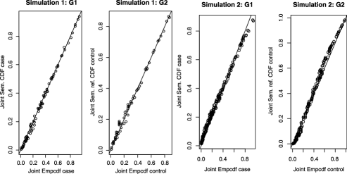
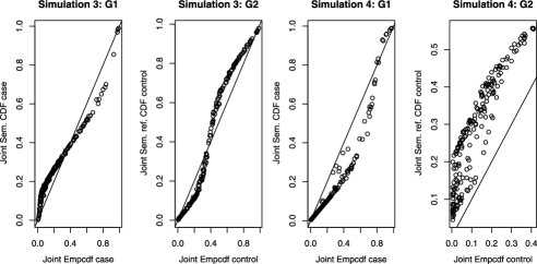
Figures 1 and 2 show the estimated and [where is the exponential tilt of defined in (22)] versus the empirical cdf and , respectively, all obtained from one run of the simulated case-control data, and evaluated at selected points in . As expected, in cases (1) and (2), there is almost a perfect agreement between versus , whereas Figure 2 shows clearly that the density ratio model is not appropriate for the data from cases () and ().
A comparison of and obtained from runs is given in Table 1. It seems that is sensitive to outliers and can give low values even for data that follow the density ratio model [e.g., case (2)]. On the other hand, the proposed measure classifies correctly the four cases, giving high values for simulations () and (2) and low values for (3) and (4). The values of in Table 1 were calculated with and . We observed that, by lowering , gets closer to for cases (3) and (4).
=185pt Run Group (1) Case 0.6307 Control 0.5976 (2) Case 0.3912 Control 0.3766 (3) Case 0.1080 Control 0.1129 (4) Case 0.0507 Control 0.0495
=185pt Case Control BW BW Simulation 1 0.46 0.47 Simulation 2 0.33 0.51
| Case | Control | |||||
| Same BW | Diff. BWs | Same BW | Diff. BWs | |||
| Simulation 1 | 0.61 | 0.90 | 0.40 | 0.59 | 0.31 | 0.61 |
| Simulation 2 | 0.38 | 0.50 | 0.20 | 0.61 | 0.36 | 0.71 |
As noted earlier, calculating the semiparametric for cases (1) and (2) entails bandwidth selection, which can be done either via the asymptotically optimal formula (4) in Voulgaraki, Kedem and Graubard (2012), replacing with (parameters estimated from the data), or via cross-validation and minimize either (3.3) or (3.3) (which also allows different bandwidths to smooth the different terms). Tables 2–4 summarize the results for the estimated bandwidths for one run of the simulations, using equations (4) in Voulgaraki, Kedem and Graubard (2012), (3.3) and (3.3). The integrals in (4) in Voulgaraki, Kedem and Graubard (2012) were calculated using Mathematica. There were no significant differences in the regression results using single or multiple bandwidths.
Using the semiparametric model, the standard normal distribution for the kernel and (24), we estimated for a single predictor. Table 5 provides MSE and MAE comparisons between the different methods for the first two simulations. In the table SP stands for semiparametric regression, MR for multiple regression, GAM for generalized additive model and NW for Nadaraya–Watson. We did not estimate for simulations and because the semiparametric model is not applicable in these cases (and was rejected as we saw from the comparisons). In simulations –, for both case and control, we fitted a thin plate regression spline GAM assuming the normal distribution and identity link. The results for tensor product were almost identical. In simulation the GAM line was almost identical to the multiple regression line. We see that the semiparametric regression performs comparably with the other methods in terms of MSE and MAE.
| Case | Control | |||||
| Same BW | Diff. BWs | Same BW | Diff. BWs | |||
| Simulation 1 | 0.64 | 0.90 | 0.50 | 0.63 | 0.21 | 0.71 |
| Simulation 2 | 0.30 | 0.40 | 0.20 | 0.74 | 0.11 | 0.96 |
| MSE | MAE | ||||||||
|---|---|---|---|---|---|---|---|---|---|
| SP | MR | GAM | NW | SP | MR | GAM | NW | ||
| Simulation 1 | 0.913 | 0.834 | 0.834 | 0.851 | 0.752 | 0.741 | 0.741 | 0.736 | |
| 0.856 | 0.892 | 0.892 | 0.849 | 0.750 | 0.786 | 0.786 | 0.740 | ||
| Simulation 2 | 0.820 | 0.841 | 0.799 | 0.792 | 0.723 | 0.730 | 0.709 | 0.704 | |
| 1.740 | 1.482 | 1.429 | 1.388 | 1.001 | 0.992 | 0.958 | 0.946 | ||
6 Application to testicular germ cell cancer
Testicular germ cell tumor (TGCT) is a common cancer among U.S. men, mainly in the age group of 15–35 years [McGlynn et al. (2003)]. In McGlynn et al. (2007) it was shown that increased risk was significantly related to height, whereas body mass index was not significant. In Kedem et al. (2009), using the two-dimensional semiparametric model, it was shown that jointly height and weight are significant risk factors. The TGCT data consist of age (years), height (cm) and weight (kg) of individuals, of which are cases and belong to the control group. We considered two cases: the 2D TGCT data set with variables height and weight and the 3D TGCT data set with variables height, weight and age. In both cases the control distribution was the reference distribution.
Equation (4) in Voulgaraki, Kedem and Graubard (2012), (3.3), (3.3) with kernel and were used to calculate the different bandwidths. The three methods gave similar results. For the 2D TGCT data set, the case bandwidths were and for height and weight, respectively, whereas, for control, we used and . For the 3D TGCT the bandwidths were for control and for case.
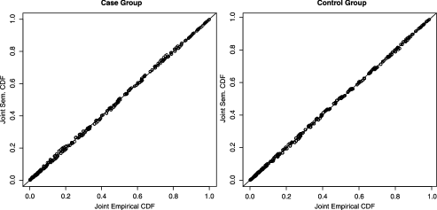
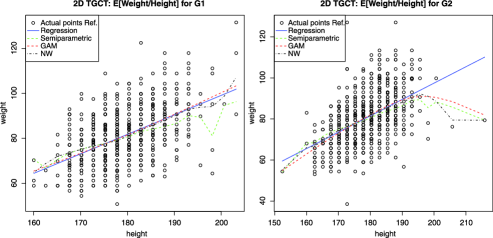
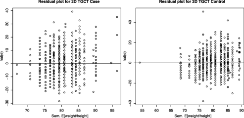
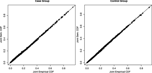
Before applying the three-dimensional density ratio model to the TGCT data, it is interesting to apply the two-dimensional model to get a prediction of weight given height only. As Figure 3 shows, the density ratio model is a suitable model for the TGCT data: there is almost a perfect agreement between the plots of the semiparametric and the corresponding empirical , . The value of is for both case and control. Figure 4 shows the estimated using (24) for the case and control groups, where in the 2D TGCT data set is weight and is height. Superimposed are the regression lines obtained from linear regression under the normal assumption, GAM and the Nadaraya–Watson regression. For the 2D TGCT data, assuming normal distribution and identity link, we fitted a tensor product GAM; there were essentially no differences between the different kinds of splines. We notice that all models give similar results. The residual plots for the semiparametric model in Figure 5 are centered around zero.
Next we fitted the 3D TGCT data with variables age, height and weight. The semiparametric model is an appropriate model for this data set as Figure 6 shows. The value of is for both case and control. An advantage of the method is that it gives estimates for the joint probabilities of age, height and weight in both case and control groups as in Table 6. The table shows the two groups are moderately different.
=320pt Probability Case Control Pr(A 45, H 152.40, W 58.967) 0.000378 0.000767 Pr(A 26, H 165.10, W 58.967) 0.004502 0.007074 Pr(A 29, H 177.80, W 65.317) 0.042723 0.054313 Pr(A 33, H 185.42, W 70.307) 0.157968 0.184774 Pr(A 34, H 180.34, W 79.832) 0.316077 0.362967 Pr(A 37, H 180.34, W 89.811) 0.513664 0.575512 Pr(A 40, H 187.96, W 94.801) 0.797157 0.833803 Pr(A 43, H 200.66, W 99.790) 0.943058 0.956300 Pr(A 45, H 203.20, W 117.934) 0.995010 0.996560
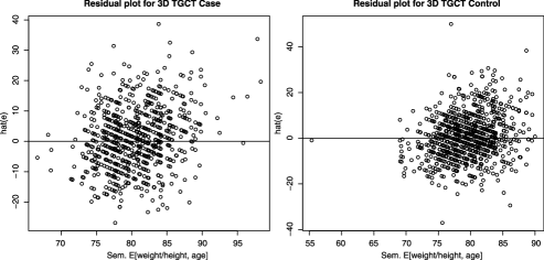
In order to calculate for the case and control groups, we used (24), where in the 3D TGCT data set is weight and represents jointly height and age. Figure 7 shows the residual plots for the semiparametric model. Table 7 gives the MSE and MAE comparison between the different regression methods for the 2D and the 3D TGCT data. For the 3D TGCT data, assuming normal distribution and identity link, we fitted a thin plate regression spline GAM because it produced better looking residual and Q–Q plots. The semiparametric regression performs comparably with the other estimators, although it has a somewhat higher MSE. These results can be explained by the fact that our method consists of an extra step of density estimation. However, we have the extra advantage that we also obtain joint probabilities of the variables, unlike multiple regression and GAM.
| MSE | MAE | ||||||||
|---|---|---|---|---|---|---|---|---|---|
| SP | MR | GAM | NW | SP | MR | GAM | NW | ||
| 2D TGCT | 99.510 | 99.250 | 98.648 | 7.947 | 7.784 | 7.770 | 7.774 | ||
| 92.264 | 90.284 | 90.332 | 7.347 | 7.296 | 7.246 | 7.241 | |||
| 3D TGCT | 96.367 | 96.091 | 89.124 | 7.770 | 7.679 | 7.672 | 7.390 | ||
| 90.291 | 88.147 | 86.932 | 7.280 | 7.244 | 7.173 | 7.139 | |||
Tables 8 and 9 give some predicted values for weight given age and height for the two groups. The results from the different methods are not much different.
We end this section by providing in (24) to help the reader interpret the results of the semiparametric analysis. Tables 10 and 11 give the case-control weight predictions (24) and the actual weights. From the tables, as expected, in (24) tends to be close to the average of ’s which correspond to the same . Empty entries in the table correspond to subjects with the same height and age (i.e., same ), but possibly different weights. The averaging property can be seen by averaging the run of weights in the “empty cells” and the run “upper point.” Thus, for example, the control-weights corresponding to age and height average to and the prediction is 76.62195. Across different ages, except for heights less than 167.64 cm, the estimated conditional expectation in cases consistently has greater body weights than controls, indicating that later life exposures such as increased caloric diet intake and/or reduced energy expenditure and lack of physical exercise may increase the risk of testicular cancer.
7 Summary
In this paper we have shown that using our proposed semi-parametric regression method we can detect an important increased risk of germ cell testicular cancer with greater body weight after adjusting for age and height that was not found with these same data using standard logistic regression modeling. This is an important finding because body weight is likely a later life exposure involving dietary caloric intake and/or energy expenditure from physical activity. This is in contrast to height that is influenced by early life factors such as genetics, early life nutrition or endogenous or exogenous hormones. The possibility of intervening to reduce body weight among young men could help to stem the rise in incidence of testicular cancer.
| Case | ||||||
|---|---|---|---|---|---|---|
| Age | Height | Weight | SP | MR | GAM | NW |
| 26 | 193.04 | 89.81775 | 92.47554 | 92.80697 | 95.96000 | |
| 24 | 167.64 | 73.59282 | 70.00329 | 70.68805 | 71.90371 | |
| 29 | 180.34 | 81.41551 | 82.42360 | 82.17237 | 81.60395 | |
| 38 | 185.42 | 86.29762 | 89.46406 | 89.50287 | 89.70666 | |
| 34 | 195.58 | 89.03635 | 97.03194 | 98.08814 | 92.45555 | |
| 27 | 162.56 | 68.53652 | 66.51540 | 67.76775 | 65.18988 | |
| Control | ||||||
|---|---|---|---|---|---|---|
| Age | Height | Weight | SP | MR | GAM | NW |
| 29 | 180.34 | 82.06293 | 82.35544 | |||
| 39 | 175.26 | 80.36549 | 80.05940 | |||
| 19 | 172.72 | 73.58821 | 73.40060 | |||
| 33 | 177.80 | 80.97707 | 81.14195 | |||
| 31 | 190.50 | 90.67494 | 87.47080 | |||
| 25 | 165.10 | 68.90777 | 69.49050 | |||
The semiparametric regression approach taken in this paper requires first efficient estimation of multivariate distributions. This can be achieved under the multidimensional density ratio model, given multiple data sources of multivariate data, and known tilts up to unknown parameters. Subject to this construct, the method produces more efficient kernel density estimators than the traditional single-sample kernel density estimator. This is so since all the finite and infinite-dimensional parameters are estimated from the entire combined data from all sources, and not just from single sources. As in the traditional kernel estimation, our kernel estimates require bandwidths and we have discussed ways for obtaining optimal and nearly optimal kernel bandwidths. The process of fitting the density ratio model and obtaining estimates is quite straightforward and quick. In this regard, several diagnostic measures have been suggested.
| Control | Case | ||||
|---|---|---|---|---|---|
| Age | Height | Weight | Weight | ||
| 27 | 162.56 | 58.967 | 69.08335 | ||
| 28 | 162.56 | 77.111 | 69.05132 | ||
| 68.039 | |||||
| 30 | 165.10 | 68.039 | 72.20524 | ||
| 37 | 165.10 | 69.40 | 72.42138 | ||
| 25 | 167.64 | 86.183 | 73.68129 | ||
| 30 | 167.64 | 72.575 | 74.81333 | ||
| 18 | 170.18 | 61.235 | 73.67032 | ||
| 32 | 170.18 | 70.307 | 76.53351 | ||
| 63.503 | |||||
| 37 | 172.72 | 74.843 | 77.88598 | ||
| 40 | 172.72 | 70.307 | 77.97789 | ||
| 77.111 | |||||
| 22 | 175.26 | 77.111 | 76.62195 | ||
| 65.771 | |||||
| 79.379 | |||||
| 83.915 | |||||
| 65.771 | |||||
| 25 | 175.26 | 68.039 | 77.14234 | ||
| 83.915 | |||||
| 74.843 | |||||
| 83.915 | |||||
| 79.379 | |||||
| 86.183 | |||||
| 26 | 177.80 | 79.379 | 78.74752 | ||
| 81.647 | |||||
| 58.967 | |||||
| 81.647 | |||||
| 79.379 | |||||
| 74.843 | |||||
| 88.451 | |||||
| 68.039 | |||||
| 42 | 177.80 | 70.307 | 80.50100 | ||
| Control | Case | ||||
|---|---|---|---|---|---|
| Age | Height | Weight | Weight | ||
| 20 | 180.34 | 79.17623 | |||
| 33 | 180.34 | 81.92536 | |||
| 18 | 182.88 | 80.23013 | |||
| 41 | 182.88 | 83.65558 | |||
| 19 | 185.42 | 81.45580 | |||
| 21 | 185.42 | 82.46773 | |||
| 22 | 190.50 | 85.23493 | |||
| 31 | 190.50 | 86.05980 | |||
| 22 | 193.04 | 86.73352 | |||
| 24 | 193.04 | 87.50020 | |||
| 34 | 193.04 | 87.72937 | |||
| 34 | 195.58 | 88.81524 | |||
Going a step further, the estimated distributions can be used in estimating joint probabilities, in ANOVA-like problems of determining differences between groups, and in estimating the conditional expectation of a response variable given random covariates, provided that multiple data sources are available. An application to predicting weight from height and age in a case-control problem shows the method competes well with several well-known regression methods, and at the same time it provides estimates of joint probabilities. Our experience suggests that the method is effective for a small number of covariates. Computational problems can arise as the number of variables increases.
We have made some numerical comparisons with GAM, but a general comparison is not our focus or intention in the present paper. Still, a few points are in order. From our limited comparison it seems the two methods produce similar regression estimates, and both methods are more complex than multiple regression. The complexity of GAM stems from their iterative nature, which is reminiscent of fixed point problems in repeated parametric filtering where estimates are evaluated at estimates iteratively, and this may affect the interpretability of the results [Li and Song (2002)]. It seems to us that the semiparametric approach, on the other hand, is somewhat more straightforward. We have illustrated in the TGCT data analysis that the resulting semiparametric regression estimate is indeed close to the average of the response conditional on fixed covariates, as one would expect. This property is shared by GAM as well. GAM assume additivity. On the other hand, the density ratio approach requires an assumption about the tilts. The suggested diagnostic tools shed light, albeit indirectly, on the appropriateness of the tilts.
Appendix
Acknowledgments
The authors wish to thank the referees and the Area Editor for their dedication, effort and important suggestions.
Supplement to “Semiparametric regression in testicular germ cell data” \slink[doi]10.1214/12-AOAS552SUPP \slink[url]http://lib.stat.cmu.edu/aoas/552/supplement.pdf \sdatatype.pdf \sdescriptionThe supplementary material contains all the mathematical proofs of the lemmas, corrolaries and theorems supporting the statements and results, including some additional references.
References
- Anderson (1971) {bbook}[auto:STB—2012/04/24—10:30:10] \bauthor\bsnmAnderson, \bfnmT. W.\binitsT. W. (\byear1971). \btitleAn Introduction to Multivariate Statistical Analysis. \bpublisherWiley, \baddressNew York. \bptokimsref \endbibitem
- Bondell (2007) {barticle}[mr] \bauthor\bsnmBondell, \bfnmHoward D.\binitsH. D. (\byear2007). \btitleTesting goodness-of-fit in logistic case-control studies. \bjournalBiometrika \bvolume94 \bpages487–495. \biddoi=10.1093/biomet/asm033, issn=0006-3444, mr=2380573 \bptokimsref \endbibitem
- Cheng and Chu (2004) {barticle}[mr] \bauthor\bsnmCheng, \bfnmK. F.\binitsK. F. and \bauthor\bsnmChu, \bfnmC. K.\binitsC. K. (\byear2004). \btitleSemiparametric density estimation under a two-sample density ratio model. \bjournalBernoulli \bvolume10 \bpages583–604. \biddoi=10.3150/bj/1093265631, issn=1350-7265, mr=2076064 \bptokimsref \endbibitem
- Fokianos (2004) {barticle}[mr] \bauthor\bsnmFokianos, \bfnmKonstantinos\binitsK. (\byear2004). \btitleMerging information for semiparametric density estimation. \bjournalJ. R. Stat. Soc. Ser. B Stat. Methodol. \bvolume66 \bpages941–958. \biddoi=10.1111/j.1467-9868.2004.05480.x, issn=1369-7412, mr=2102474 \bptokimsref \endbibitem
- Fokianos et al. (2001) {barticle}[mr] \bauthor\bsnmFokianos, \bfnmKonstantinos\binitsK., \bauthor\bsnmKedem, \bfnmBenjamin\binitsB., \bauthor\bsnmQin, \bfnmJing\binitsJ. and \bauthor\bsnmShort, \bfnmDavid A.\binitsD. A. (\byear2001). \btitleA semiparametric approach to the one-way layout. \bjournalTechnometrics \bvolume43 \bpages56–65. \biddoi=10.1198/00401700152404327, issn=0040-1706, mr=1819908 \bptokimsref \endbibitem
- Gilbert (2004) {barticle}[mr] \bauthor\bsnmGilbert, \bfnmPeter B.\binitsP. B. (\byear2004). \btitleGoodness-of-fit tests for semiparametric biased sampling models. \bjournalJ. Statist. Plann. Inference \bvolume118 \bpages51–81. \biddoi=10.1016/S0378-3758(02)00405-6, issn=0378-3758, mr=2015221 \bptokimsref \endbibitem
- Gilbert, Lele and Vardi (1999) {barticle}[mr] \bauthor\bsnmGilbert, \bfnmPeter B.\binitsP. B., \bauthor\bsnmLele, \bfnmSubhash R.\binitsS. R. and \bauthor\bsnmVardi, \bfnmYehuda\binitsY. (\byear1999). \btitleMaximum likelihood estimation in semiparametric selection bias models with application to AIDS vaccine trials. \bjournalBiometrika \bvolume86 \bpages27–43. \biddoi=10.1093/biomet/86.1.27, issn=0006-3444, mr=1688069 \bptokimsref \endbibitem
- Hastie and Tibshirani (1990) {bbook}[mr] \bauthor\bsnmHastie, \bfnmT. J.\binitsT. J. and \bauthor\bsnmTibshirani, \bfnmR. J.\binitsR. J. (\byear1990). \btitleGeneralized Additive Models. \bseriesMonographs on Statistics and Applied Probability \bvolume43. \bpublisherChapman and Hall, \baddressLondon. \bidmr=1082147 \bptokimsref \endbibitem
- Kedem et al. (2008) {barticle}[mr] \bauthor\bsnmKedem, \bfnmBenjamin\binitsB., \bauthor\bsnmLu, \bfnmGuanhua\binitsG., \bauthor\bsnmWei, \bfnmRong\binitsR. and \bauthor\bsnmWilliams, \bfnmPaul D.\binitsP. D. (\byear2008). \btitleForecasting mortality rates via density ratio modeling. \bjournalCanad. J. Statist. \bvolume36 \bpages193–206. \biddoi=10.1002/cjs.5550360202, issn=0319-5724, mr=2522160 \bptokimsref \endbibitem
- Kedem et al. (2009) {barticle}[mr] \bauthor\bsnmKedem, \bfnmBenjamin\binitsB., \bauthor\bsnmKim, \bfnmEun-young\binitsE.-y., \bauthor\bsnmVoulgaraki, \bfnmAnastasia\binitsA. and \bauthor\bsnmGraubard, \bfnmBarry I.\binitsB. I. (\byear2009). \btitleTwo-dimensional semiparametric density ratio modeling of testicular germ cell data. \bjournalStat. Med. \bvolume28 \bpages2147–2159. \biddoi=10.1002/sim.3611, issn=0277-6715, mr=2751511 \bptokimsref \endbibitem
- Li and Song (2002) {barticle}[mr] \bauthor\bsnmLi, \bfnmTa-Hsin\binitsT.-H. and \bauthor\bsnmSong, \bfnmKai-Sheng\binitsK.-S. (\byear2002). \btitleAsymptotic analysis of a fast algorithm for efficient multiple frequency estimation. \bjournalIEEE Trans. Inform. Theory \bvolume48 \bpages2709–2720. \biddoi=10.1109/TIT.2002.802635, issn=0018-9448, mr=1930338 \bptokimsref \endbibitem
- Lu (2007) {bmisc}[mr] \bauthor\bsnmLu, \bfnmGuanhua\binitsG. (\byear2007). \bhowpublishedAsymptotic theory for multiple-sample semiparpametric density ratio models and its application to mortality forecasting. Ph.D. dissertation, Univ. Maryland, College Park, MD. \bidmr=2711353 \bptokimsref \endbibitem
- McGlynn and Cook (2010) {bincollection}[auto:STB—2012/04/24—10:30:10] \bauthor\bsnmMcGlynn, \bfnmK. A.\binitsK. A. and \bauthor\bsnmCook, \bfnmM. B.\binitsM. B. (\byear2010). \btitleThe epidemiology of testicular cancer. In \bbooktitleMale Reproductive Cancers: Epidemiology, Pathology and Genetics (\beditor\bfnmW. D.\binitsW. D. \bsnmFoulkes and \beditor\bfnmK. A.\binitsK. A. \bsnmCooney, eds.) \bpages51–83. \bpublisherSpringer, \baddressNew York. \bptokimsref \endbibitem
- McGlynn et al. (2003) {barticle}[pbm] \bauthor\bsnmMcGlynn, \bfnmKatherine A.\binitsK. A., \bauthor\bsnmDevesa, \bfnmSusan S.\binitsS. S., \bauthor\bsnmSigurdson, \bfnmAlice J.\binitsA. J., \bauthor\bsnmBrown, \bfnmLinda M.\binitsL. M., \bauthor\bsnmTsao, \bfnmLilian\binitsL. and \bauthor\bsnmTarone, \bfnmRobert E.\binitsR. E. (\byear2003). \btitleTrends in the incidence of testicular germ cell tumors in the United States. \bjournalCancer \bvolume97 \bpages63–70. \biddoi=10.1002/cncr.11054, issn=0008-543X, pmid=12491506 \bptokimsref \endbibitem
- McGlynn et al. (2007) {barticle}[auto:STB—2012/04/24—10:30:10] \bauthor\bsnmMcGlynn, \bfnmK. A.\binitsK. A., \bauthor\bsnmSakoda1, \bfnmL. C.\binitsL. C., \bauthor\bsnmRubertone, \bfnmM. V.\binitsM. V., \bauthor\bsnmSesterhenn, \bfnmI. A.\binitsI. A., \bauthor\bsnmLyu, \bfnmC.\binitsC., \bauthor\bsnmGraubard, \bfnmB. I.\binitsB. I. and \bauthor\bsnmErickson, \bfnmR. L.\binitsR. L. (\byear2007). \btitleBody size, dairy consumption, puberty, and risk of testicular germ cell tumors. \bjournalAmerican Journal of Epidemiology \bvolume165 \bpages355–363. \bptokimsref \endbibitem
- Nadaraya (1964) {barticle}[auto:STB—2012/04/24—10:30:10] \bauthor\bsnmNadaraya, \bfnmE. A.\binitsE. A. (\byear1964). \btitleOn estimating regression. \bjournalTheory Probab. Appl. \bvolume9 \bpages141–142. \bptokimsref \endbibitem
- Ogden et al. (2004) {barticle}[pbm] \bauthor\bsnmOgden, \bfnmCynthia L.\binitsC. L., \bauthor\bsnmFryar, \bfnmCheryl D.\binitsC. D., \bauthor\bsnmCarroll, \bfnmMargaret D.\binitsM. D. and \bauthor\bsnmFlegal, \bfnmKatherine M.\binitsK. M. (\byear2004). \btitleMean body weight, height, and body mass index, United States 1960–2002. \bjournalAdv. Data \bvolume347 \bpages1–17. \bidissn=0147-3956, pmid=15544194 \bptokimsref \endbibitem
- Parzen (1962) {barticle}[mr] \bauthor\bsnmParzen, \bfnmEmanuel\binitsE. (\byear1962). \btitleOn estimation of a probability density function and mode. \bjournalAnn. Math. Statist. \bvolume33 \bpages1065–1076. \bidissn=0003-4851, mr=0143282 \bptokimsref \endbibitem
- Phue et al. (2007) {barticle}[pbm] \bauthor\bsnmPhue, \bfnmJe-Nie\binitsJ.-N., \bauthor\bsnmKedem, \bfnmBenjamin\binitsB., \bauthor\bsnmJaluria, \bfnmPratik\binitsP. and \bauthor\bsnmShiloach, \bfnmJoseph\binitsJ. (\byear2007). \btitleEvaluating microarrays using a semiparametric approach: Application to the central carbon metabolism of Escherichia coli BL21 and JM109. \bjournalGenomics \bvolume89 \bpages300–305. \biddoi=10.1016/j.ygeno.2006.10.004, issn=0888-7543, mid=NIHMS16517, pii=S0888-7543(06)00298-9, pmcid=1945183, pmid=17125967 \bptnotecheck year\bptokimsref \endbibitem
- Prentice and Pyke (1979) {barticle}[mr] \bauthor\bsnmPrentice, \bfnmR. L.\binitsR. L. and \bauthor\bsnmPyke, \bfnmR.\binitsR. (\byear1979). \btitleLogistic disease incidence models and case-control studies. \bjournalBiometrika \bvolume66 \bpages403–411. \biddoi=10.1093/biomet/66.3.403, issn=0006-3444, mr=0556730 \bptokimsref \endbibitem
- Qin (1998) {barticle}[mr] \bauthor\bsnmQin, \bfnmJing\binitsJ. (\byear1998). \btitleInferences for case-control and semiparametric two-sample density ratio models. \bjournalBiometrika \bvolume85 \bpages619–630. \biddoi=10.1093/biomet/85.3.619, issn=0006-3444, mr=1665814 \bptokimsref \endbibitem
- Qin and Lawless (1994) {barticle}[mr] \bauthor\bsnmQin, \bfnmJing\binitsJ. and \bauthor\bsnmLawless, \bfnmJerry\binitsJ. (\byear1994). \btitleEmpirical likelihood and general estimating equations. \bjournalAnn. Statist. \bvolume22 \bpages300–325. \biddoi=10.1214/aos/1176325370, issn=0090-5364, mr=1272085 \bptokimsref \endbibitem
- Qin and Zhang (1997) {barticle}[mr] \bauthor\bsnmQin, \bfnmJing\binitsJ. and \bauthor\bsnmZhang, \bfnmBiao\binitsB. (\byear1997). \btitleA goodness-of-fit test for logistic regression models based on case-control data. \bjournalBiometrika \bvolume84 \bpages609–618. \biddoi=10.1093/biomet/84.3.609, issn=0006-3444, mr=1603924 \bptokimsref \endbibitem
- Qin and Zhang (2005) {barticle}[mr] \bauthor\bsnmQin, \bfnmJing\binitsJ. and \bauthor\bsnmZhang, \bfnmBiao\binitsB. (\byear2005). \btitleDensity estimation under a two-sample semiparametric model. \bjournalJ. Nonparametr. Stat. \bvolume17 \bpages665–683. \biddoi=10.1080/10485250500039346, issn=1048-5252, mr=2165095 \bptokimsref \endbibitem
- Rencher (2000) {bbook}[mr] \bauthor\bsnmRencher, \bfnmAlvin C.\binitsA. C. (\byear2000). \btitleLinear Models in Statistics. \bpublisherWiley, \baddressNew York. \bidmr=1719141 \bptokimsref \endbibitem
- Shao (2003) {bbook}[mr] \bauthor\bsnmShao, \bfnmJun\binitsJ. (\byear2003). \btitleMathematical Statistics, \bedition2nd ed. \bpublisherSpringer, \baddressNew York. \biddoi=10.1007/b97553, mr=2002723 \bptokimsref \endbibitem
- Silverman (1986) {bbook}[mr] \bauthor\bsnmSilverman, \bfnmB. W.\binitsB. W. (\byear1986). \btitleDensity Estimation for Statistics and Data Analysis. \bpublisherChapman and Hall, \baddressLondon. \bidmr=0848134 \bptokimsref \endbibitem
- Voulgaraki, Kedem and Graubard (2012) {bmisc}[auto:STB—2012/04/24—10:30:10] \bauthor\bsnmVoulgaraki, \bfnmA.\binitsA., \bauthor\bsnmKedem, \bfnmB.\binitsB. and \bauthor\bsnmGraubard, \bfnmB. I.\binitsB. I. (\byear2012). \bhowpublishedSupplement to “Semiparametric regression in testicular germ cell data.” DOI:\doiurl10.1214/12-AOAS552SUPP. \bptokimsref \endbibitem
- Watson (1964) {barticle}[mr] \bauthor\bsnmWatson, \bfnmGeoffrey S.\binitsG. S. (\byear1964). \btitleSmooth regression analysis. \bjournalSankhyā Ser. A \bvolume26 \bpages359–372. \bidissn=0581-572X, mr=0185765 \bptokimsref \endbibitem
- Wen and Kedem (2009) {barticle}[auto:STB—2012/04/24—10:30:10] \bauthor\bsnmWen, \bfnmS.\binitsS. and \bauthor\bsnmKedem, \bfnmB.\binitsB. (\byear2009). \btitleA semiparametric cluster detection method—a comprehensive power comparison with Kulldorff’s method. \bjournalInternational Journal of Health Geographics \bvolume8. \bnoteOnline journal without page numbers. \bptokimsref \endbibitem
- Wood (2006) {bbook}[mr] \bauthor\bsnmWood, \bfnmSimon N.\binitsS. N. (\byear2006). \btitleGeneralized Additive Models: An Introduction With R. \bpublisherChapman & Hall/CRC, \baddressBoca Raton, FL. \bidmr=2206355 \bptokimsref \endbibitem
- Zhang (1999) {barticle}[mr] \bauthor\bsnmZhang, \bfnmBiao\binitsB. (\byear1999). \btitleA chi-squared goodness-of-fit test for logistic regression models based on case-control data. \bjournalBiometrika \bvolume86 \bpages531–539. \biddoi=10.1093/biomet/86.3.531, issn=0006-3444, mr=1723776 \bptokimsref \endbibitem
- Zhang (2000) {barticle}[mr] \bauthor\bsnmZhang, \bfnmBiao\binitsB. (\byear2000). \btitleA goodness of fit test for multiplicative-intercept risk models based on case-control data. \bjournalStatist. Sinica \bvolume10 \bpages839–865. \bidissn=1017-0405, mr=1787782 \bptokimsref \endbibitem
- Zhang (2001) {barticle}[mr] \bauthor\bsnmZhang, \bfnmBiao\binitsB. (\byear2001). \btitleAn information matrix test for logistic regression models based on case-control data. \bjournalBiometrika \bvolume88 \bpages921–932. \biddoi=10.1093/biomet/88.4.921, issn=0006-3444, mr=1872210 \bptokimsref \endbibitem
- Zhang (2002) {barticle}[mr] \bauthor\bsnmZhang, \bfnmBiao\binitsB. (\byear2002). \btitleAssessing goodness-of-fit of generalized logit models based on case-control data. \bjournalJ. Multivariate Anal. \bvolume82 \bpages17–38. \biddoi=10.1006/jmva.2001.2019, issn=0047-259X, mr=1918613 \bptokimsref \endbibitem