A Numerical Test of a High-Penetrability Approximation for the One-Dimensional Penetrable-Square-Well Model

Abstract

The one-dimensional penetrable-square-well fluid is studied using both analytical tools and specialized Monte Carlo simulations. The model consists of a penetrable core characterized by a finite repulsive energy combined with a short-range attractive well. This is a many-body one-dimensional problem, lacking an exact analytical solution, for which the usual van Hove theorem on the absence of phase transition does not apply. We determine a high-penetrability approximation complementing a similar low-penetrability approximation presented in previous work. This is shown to be equivalent to the usual Debye–Hückel theory for simple charged fluids for which the virial and energy routes are identical. The internal thermodynamic consistency with the compressibility route and the validity of the approximation in describing the radial distribution function is assessed by a comparison against numerical simulations. The Fisher–Widom line separating the oscillatory and monotonic large-distance behavior of the radial distribution function is computed within the high-penetrability approximation and compared with the opposite regime, thus providing a strong indication of the location of the line in all possible regimes. The high-penetrability approximation predicts the existence of a critical point and a spinodal line, but this occurs outside the applicability domain of the theory. We investigate the possibility of a fluid-fluid transition by Gibbs ensemble Monte Carlo techniques, not finding any evidence of such a transition. Additional analytical arguments are given to support this claim. Finally, we find a clustering transition when Ruelle’s stability criterion is not fulfilled. The consequences of these findings on the three-dimensional phase diagrams are also discussed.

I Introduction

Recent advances in chemical synthesis have unveiled more and more the importance of soft-matter systems, such as dispersions of colloidal particles, polymers, and their combinations. Besides their practical interest, these new developments have opened up new theoretical avenues in (at least) two instances. Firstly, it is possible to experimentally fine-tune the details of interactions (range, strength, …), making these systems a unique laboratory for testing highly simplified models within an effective-interaction approach where the microscopic degrees of freedom are integrated out in favor of renormalized macroparticle interactions. Secondly, they offer the possibility of exploring new types of equilibrium phase behaviors not present in the simple-fluid paradigm.

As early as in 1989, Marquest and WittenMarquest89 suggested that the experimentally observed crystallization in some copolymer micellar systems could be rationalized on the basis of a bounded interaction, that is, an interaction that does not diverge at the origin. Successive theoretical work showed that this class of bounded or ultra-soft potentials naturally arises as effective interactions between the centers of mass of many soft and flexible macromolecules, such as polymer chains, dendrimers, star polymers, etc. (see, e.g., Ref. Likos01, for a reference on the subject). Two well-studied cases belonging to the above class are the Gaussian core model (GCM) introduced by StillingerStillinger76 and the penetrable-sphere (PS) model introduced in Refs. Marquest89, ; Likos98, , whose freezing transition turns out to display rather exotic features with no analogue in the atomistic fluid realm.

In the present paper, we shall consider a close relative of the PS model, first introduced in Ref. Santos08, , denoted as the penetrable-square-well (PSW) model, where a short-range attractive tail is added to the PS model just outside the core region. In the limit of infinite repulsive energy, the PS and PSW models reduce to the usual hard-sphere (HS) and square-well (SW) models, respectively.

An additional interesting feature common to both PS and PSW, as well as to all bounded potentials, is the fact that, even when confined to one-dimensional systems, they may exhibit a non-trivial phase diagram due to the penetrability which prevents an exact analytical solution.

This is because particles cannot be lined up on a line with a well-defined and fixed ordering in view of the possibility of reciprocal interpenetration (with some positive energy cost), thus lacking an essential ingredient allowing for an exact solution in the respective hard-core counterparts (HS and SW). It is then particularly useful to discuss some motivated approximations in the one-dimensional model which can then be benchmarked against numerical simulations and subsequently exploited in the much more complex three-dimensional case.

The aim of the present paper is to complete a study on the one-dimensional PSW model started in Refs. Santos08, ; Fantoni09, , as well as the general results presented in Ref. Santos08, which are particularly relevant in the present context. In the first paper of the series,Santos08 we introduced the model and discussed the range of stability in terms of the attractive versus repulsive energy scale. We provided, in addition, exact analytical results in the low-density limit (second order in the radial distribution function and fourth order in the virial expansion) and a detailed study of the Percus–Yevick and hypernetted-chain integral equations. These were used in the following paperFantoni09 to propose a low-penetrability approximation at finite density which was then tested against numerical simulation. This low-penetrability approximation is expected to break down in the opposite regime, namely when temperatures and densities are such that particles easily interpenetrate each other. In the present paper, we address this latter regime by proposing a complementary approximation (the high-penetrability approximation) and discussing its range of validity and the relationship with the low-penetrability regime. Note that a similar matching of the low- and high-penetrability approximation has already been carried out by two of the present authors in the framework of the PS model.Malijevsky06 ; MYS07 It turns out that the high-penetrability approximation in the context of bounded potentials coincides with the linearized Debye–Hückel classical approximation originally introduced in the framework of the Coulomb potential.Hansen86 It has been recently shownSantos09 that two of the three standard routes to thermodynamics (the energy and the virial routes) are automatically consistent within the linearized Debye–Hückel approximation, for any potential and dimensionality. This means that a deviation from the third standard route to thermodynamics (the compressibility route) can be exploited to assess the degree of reliability of the high-penetrability (or linearized Debye–Hückel) approximation. This is indeed discussed in the present paper, where we also discuss the full hierarchy of approximations ranging from the full Debye–Hückel approximation to the simplest mean-spherical approximation.

In view of the boundness of the potential, the usual van Hove no-go theoremVanHove50 ; Cuesta04 on the absence of phase transitions in certain one-dimensional fluids does not hold. It is then natural to ask whether a phase transition occurs in the one-dimensional PSW fluid by noting that the addition of an attractive tail to the pair potential of the PS model extends the question to the fluid-fluid transition, in addition to the fluid-solid transition possible even within the PS model. In the present paper we confine our attention to the fluid-fluid case only and discuss this possibility using both analytical arguments and state-of-the-art numerical simulations.Panagiotopoulos87 ; Panagiotopoulos88 ; Smit89a ; Smit89b Our results are compatible with the absence of such a transition, as we shall discuss. This is also supported by recent analytical resultsFantoni10 using a methodology devised for one-dimensional models with long-range interactions.Kastner08 We discuss possible reasons for this and a plausible scenario for the three-dimensional case.

Finally, we note that the approach to a critical point is frequently anticipated by the so-called Fisher–Widom lineFisher69 marking the borderline between a region with oscillatory behavior in the long-range domain of the correlation function (above the Fisher–Widom line) and a region of exponential decay. We discuss the location of this line within the high-penetrability approximation and again the matching of this result with that stemming from the low-penetrability approximation.

The structure of the paper is as follows. We define the PSW model in Sec. II. We then construct the high-penetrability approximation in Sec. III and in Sec. IV we discuss some approximations related to it. Section V contains a discussion on the routes to thermodynamics, as predicted by the high-penetrability approximation. The structure predicted by the approximation is compared with Monte Carlo data in Sec. VI. The Fisher–Widom line and the possibility of a fluid-fluid transition are discussed in Sec. VII. The paper ends with some concluding remarks in Sec. VIII.

II The penetrable-square-well (PSW) model

The penetrable-square-well (PSW) model is defined by the following pair potentialSantos08 ; Fantoni09

$$\phi_{\text{PSW}}\left(r\right)=\left\{\begin{array}[]{ll}+\epsilon_{r},&r<\sigma,\\ -\epsilon_{a},&\sigma<r<\sigma+\Delta,\\ 0,&r>\sigma+\Delta,\end{array}\right.$$ (4)

where $\Delta$ is the well width and $\epsilon_{r}$ and $\epsilon_{a}$ are two positive constants accounting for the repulsive and attractive parts of the potential, respectively. In the following, we shall restrict our analysis to the case $\Delta/\sigma<1$ and $\epsilon_{r}>2\epsilon_{a}$, where we know the one-dimensional model to be stable with a well defined thermodynamic limit.Santos08 It is shown in Appendix A that, more generally, the one-dimensional PSW model is guaranteed to be stable if ${\epsilon_{r}}>{2(\ell+1)\epsilon_{a}}$, where $\ell$ is the integer part of $\Delta/\sigma$. For lower values of $\epsilon_{r}$ the model may or may not be stable and we will come back to this point in Section VII.

An important role in the following is played by the corresponding Mayer function

$$f_{\text{PSW}}\left(r\right)=\gamma_{r}f_{\text{HS}}\left(r\right)+\gamma_{a}\left[\Theta\left(r-\sigma\right)-\Theta\left(r-\sigma-\Delta\right)\right],$$ (5)

where $\gamma_{r}=1-e^{-\beta\epsilon_{r}}$ is the parameter measuring the degree of penetrability varying between 0 (free penetrability) and 1 (impenetrability), while $\gamma_{a}=e^{\beta\epsilon_{a}}-1>0$ measures the strength of the well depth. Here $\beta=1/k_{B}T$ with $T$ the temperature and $k_{B}$ the Boltzmann constant, $f_{\text{HS}}(r)=-\Theta(\sigma-r)$ is the Mayer function for hard spheres, and $\Theta(r)$ is the Heaviside step function.

A detailed discussion of the limiting cases of the PSW model can be found in Ref. Santos08, . Here we merely note that the PSW Mayer function $f_{\text{PSW}}(r)$ is immediately related to the usual SW Mayer function by

$$f_{\text{PSW}}(r)=\gamma_{r}f_{\text{SW}}\left(r\right),$$ (6)

$$f_{\text{SW}}\left(r\right)=f_{\text{HS}}\left(r\right)+\gamma\left[\Theta\left(r-\sigma\right)-\Theta\left(r-\sigma-\Delta\right)\right]~{},$$ (7)

where we have introduced the ratio $\gamma=\gamma_{a}/\gamma_{r}$. At a given value of $\epsilon_{r}/\epsilon_{a}$, $\gamma$ increases quasi-linearly with $e^{\beta\epsilon_{a}}$, its minimum value $\gamma=\epsilon_{a}/\epsilon_{r}$ corresponding to $\beta\epsilon_{a}\to 0$.

III A High-Penetrability Approximation (HPA)

In Ref. Fantoni09, we discussed a low-penetrability approximation (LPA) to the PSW model. Within this approximation, one assumes $1-\gamma_{r}=e^{-\beta\epsilon_{r}}\ll 1$ so that the repulsive barrier $\epsilon_{r}$ is sufficiently higher than the thermal energy $k_{B}T$, penetrability is small, and the system is almost a hard-core one. The advantage of this theoretical scheme is that one can use the general recipe leading to the exact solution for the one-dimensional SW problem —in fact, valid for any potential with a hard core and short-range attractions— and perform some ad hoc adjustments to ensure that some basic physical conditions on the radial distribution function $g(r)$ are satisfied. Comparison with Monte Carlo (MC) simulations showed a good behavior of the LPA even for $\beta\epsilon_{r}=2$ ($1-\gamma_{r}\simeq 0.14$), provided the density was moderate ($\rho\sigma<0.5$).

The opposite limit $\gamma_{r}\ll 1$ is also inherently interesting for several reasons. From a physical viewpoint this amounts to starting from the ideal gas limit $\gamma_{r}\to 0$ (one of the common reference systems for simple fluids) and progressively building up interactions by increasing $\gamma_{r}$. An additional mathematical advantage stems from the simple observationMalijevsky06 ; MYS07 ; AS04 that in the (exact) cluster expansion of $g(r)$ only the dominant chain diagrams need to be retained at all orders, thus leading to the possibility of an exact summation of those leading contributions. As we shall see shortly, this is in fact a procedure known as the Debye–Hückel approximation in the context of charged fluids.Santos09 ; Hansen86

Our main goal is the computation of the cavity function $y(r)\equiv e^{\beta\phi(r)}g(r)$, from which one can immediately compute the radial distribution function (RDF) $g(r)=y(r)[1+f(r)]$. In the PSW case one then has from Eq. (6)

$$g(r) = \left\{\begin{array}[]{ll}(1-\gamma_{r})y(r),&r<1,\\ (1+\gamma_{a})y(r),&1<r<\lambda,\\ y(r),&r>\lambda.\end{array}\right.$$ (11)

where $\lambda=1+\Delta$ and, in conformity with previous work,Santos08 ; Fantoni09 we have redefined all lengths in units of $\sigma$ so we set $\sigma=1$ in most of the following equations.

As shown in Ref. AS04, for the PS case, the exact form of the PSW cavity function in the limit $\gamma_{r}\to 0$ at finite $\gamma=\gamma_{a}/\gamma_{r}$ and $\rho\gamma_{r}$ is

$$y\left(r\right) = 1+\gamma_{r}w\left(r\right)~{},$$ (12)

where the function $w(r)$ is defined through its Fourier transform

$$\widetilde{w}(k) = \rho\gamma_{r}\frac{\widetilde{f}_{\text{SW}}^{2}(k)}{1-\rho\gamma_{r}\widetilde{f}_{\text{SW}}(k)},$$ (13)

$\widetilde{f}_{\text{SW}}(k)$ being the Fourier transform of ${f}_{\text{SW}}(r)$. Note that in the limit $\gamma_{r}\to 0$ one has $\gamma_{r}\approx\beta\epsilon_{r}$ and $\gamma\approx\epsilon_{a}/\epsilon_{r}$.

Generalizing an analogous approximation in the context of the PS model,Malijevsky06 ; MYS07 our high-penetrability approximation (HPA) consists of assuming Eqs. (12) and (13) for finite, but small, values of $\gamma_{r}$. It is worth noting that the combination of the two expressions (12) and (13) defines what is usually referred to, in a different context, as the linearized Debye–Hückel (LDH) approximation,Santos09 ; Hansen86 and this will be further elaborated below.

Equations (12) and (13) hold for any dimensionality. In the specific one-dimensional case, and taking into account Eq. (7), we have

$$\widetilde{f}_{\text{SW}}\left(k\right) = 2\int_{0}^{\infty}dr\cos(kr)f_{\text{SW}}(r)$$ (14)

$$= -\frac{2}{k}\left[\left(1+\gamma\right){\sin k}-\gamma{\sin\lambda k}\right]~{}.$$

The function $w(r)$ can be numerically evaluated in real space by Fourier inversion as

$$w(r)=\frac{\rho\gamma_{r}}{\pi}\int_{0}^{\infty}dk\,\cos(kr)\frac{\widetilde{f}_{\text{SW}}^{2}(k)}{1-\rho\gamma_{r}\widetilde{f}_{\text{SW}}(k)}.$$ (15)

An explicit expression for the density expansion of $w(r)$ within the HPA is reported in Eqs. (49) and (50) of Appendix B, where the radius of convergence of the expansion is also analyzed.

From Eqs. (6), (11), and (12) the total correlation function, $h(r)=g(r)-1$, within the HPA is easily obtained as

$$h\left(r\right) = \gamma_{r}w\left(r\right)\left[1+\gamma_{r}f_{\text{SW}}\left(r\right)\right]+\gamma_{r}f_{\text{SW}}\left(r\right)~{},$$ (16)

or in Fourier space,

$$\widetilde{h}\left(k\right) = \gamma_{r}\frac{\widetilde{f}_{\text{SW}}\left(k\right)}{1-\rho\gamma_{r}\widetilde{f}_{\text{SW}}\left(k\right)}$$ (17)

$$+\rho\gamma_{r}^{3}\int_{-\infty}^{\infty}\frac{dk^{\prime}}{2\pi}\,\frac{\widetilde{f}^{2}_{\text{SW}}(k^{\prime})\widetilde{f}_{\text{SW}}(\left|k-k^{\prime}\right|)}{1-\rho\gamma_{r}\widetilde{f}_{\text{SW}}\left(k^{\prime}\right)}.$$

From this equation it is straightforward to get the structure factor

$$S(k) = 1+\rho\widetilde{h}(k)$$ (18)

$$= \frac{1}{1-\rho\gamma_{r}\widetilde{f}_{\text{SW}}\left(k\right)}$$

$$+\rho^{2}\gamma_{r}^{3}\int_{-\infty}^{\infty}\frac{dk^{\prime}}{2\pi}\,\frac{\widetilde{f}^{2}_{\text{SW}}(k^{\prime})\widetilde{f}_{\text{SW}}(\left|k-k^{\prime}\right|)}{1-\rho\gamma_{r}\widetilde{f}_{\text{SW}}\left(k^{\prime}\right)}$$

and the Fourier transform of the direct correlation function $\widetilde{c}(k)=\widetilde{h}(k)/S(k)$. The zero wavenumber value of the structure factor is

$$S(0)=\frac{1}{1+2\rho\gamma_{r}(1-\gamma\Delta)}+\rho^{2}\gamma_{r}^{3}\int_{0}^{\infty}\frac{dk}{\pi}\,\frac{\widetilde{f}^{3}_{\text{SW}}(k)}{1-\rho\gamma_{r}\widetilde{f}_{\text{SW}}\left(k\right)},$$ (19)

where we have taken into account that $\widetilde{f}_{\text{SW}}\left(0\right)=-2(1-\gamma\Delta)$. This completes the calculation of the correlation functions within the HPA.

IV Approximations related to the HPA

As anticipated in Section III, the HPA is the exact equivalent to the well-known LDH approximation, which is widely used in the context of charged simple fluids.Hansen86 The latter is actually an intermediate step of a hierarchy of successive approximations ranging from the simplest mean-spherical approximation (MSA) to the full non-linear version of the Debye–Hückel approximation (see Ref. [11] in Ref. Santos09, for a discussion on this point). For the PSW model —and more generally for any bounded potential— the LDH approximation (the HPA in the present language) is particularly relevant in view of the fact that one can make $f_{\text{PSW}}(r)$ arbitrarily small by letting $\gamma_{r}\to 0$, thus justifying the approximation of neglecting non-chain diagrams. It is then interesting to check the performance of the other approximations included in the aforementioned class, which will be translated in the present context for simplicity.

On top of the hierarchy of approximations there is the non-linear HPA (nlHPA)

$$y\left(r\right) = e^{\gamma_{r}w\left(r\right)}~{},$$ (20)

which is equivalent to the non-linear Debye–Hückel approximation, as remarked. The HPA, Eq. (12), is obtained upon linearizing the exponential, an approximation valid again in the limit $\gamma_{r}\ll 1$. An additional approximation —denoted here as the modified HPA (mHPA)— can be considered with the help of Eq. (16) by neglecting the quadratic term in $\gamma_{r}$. This yields

$$h\left(r\right) = \gamma_{r}\left[w(r)+f_{\text{SW}}\left(r\right)\right]~{}.$$ (21)

This is equivalent to keeping only the first term on the right-hand side of Eq. (17), which implies $\widetilde{c}\left(k\right)=\gamma_{r}\widetilde{f}_{\text{SW}}\left(k\right)$ or, in real space,

$$c\left(r\right) = f_{\text{PSW}}\left(r\right)~{}.$$ (22)

The lowest rank in the hierarchy is occupied by the MSA, which is obtained from Eq. (22) upon linearization of the Mayer function $f_{\text{PSW}}(r)$,

$$c\left(r\right) = -\beta\phi_{\text{PSW}}\left(r\right)~{}.$$ (23)

Since $w(r)$ is a convolution, it must be continuous at $r=1$ and $r=\lambda$. It follows that the approximations with a continuous cavity function at $r=1$ and $r=\lambda$ are nlHPA and HPA. For instance, in the mHPA (21) the cavity function is $y(r)=1+\gamma_{r}w(r)/[1+\gamma_{r}f_{\text{SW}}(r)]$, so that one has $y(1^{-})-y(1^{+})=\gamma_{r}^{2}w(1)(1+\gamma)(1-\gamma_{r})^{-1}(1+\gamma\gamma_{r})^{-1}$ and $y(\lambda^{+})-y(\lambda^{-})=\gamma_{r}^{2}w(\lambda)\gamma(1+\gamma\gamma_{r})^{-1}$.

It has been shown in Ref. Santos09, that the virial and energy routes to thermodynamics (to be discussed below) are consistent one another within the HPA, for any potential and any dimensionality. A similar statement holds true for soft potentials within the MSA.Santos07 This clearly includes the PSW potential in both cases.

It is interesting to make contact with previous work carried out by Likos et al. Likos01b ; Likos07 on a general class of unbounded potentials which are free of attractive parts, thus resulting particularly useful in the context of the fluid-solid transition. In Ref. Likos01b, , the MSA given in Eq. (23) along with the spinodal instability to be discussed in detail in Section VII, have been introduced for a general class of unbounded potentials including the PS as a particular case. This has been further elaborated and extended to include the GCM in Ref. Likos07, . In both cases, the authors discuss directly the three-dimensional case, so that a direct comparison with the present work cannot be drawn at the present stage, but they also provide a detailed discussion of various approximations, within the general framework of density functional theory, that provide a unified framework where even the present model could be included.

V Equation of state

Given an approximate solution of a fluid model there are several routes to the equation of state which, in general, give different results. The most common are three:Hansen86 the virial, the compressibility, and the energy route. The consistency of the outcome of these different routes can be regarded as an assessment on the soundness of the approximation. For some particular approximations it may also happen that the consistency of two of the three routes are automatically enforced (see Ref. Santos09, and references therein for a detailed discussion on this point). This is the case of the HPA, where the virial and energy routes coincide, as anticipated. Hence, the consistency with the compressibility route will provide a rough estimate of the regime of validity of the HPA within a phase diagram for the PSW potential.

Let us briefly recallHansen86 the methods to compute the compressibility factor, $Z=\beta p/\rho$, associated with the three different routes. The virial route is defined by

$$Z = 1-\rho\beta\int_{0}^{\infty}dr\,ry\left(r\right)e^{-\beta\phi\left(r\right)}\phi^{\prime}\left(r\right),$$ (24)

which, using standard manipulations,Hansen86 yields

$$Z = 1+\rho\gamma_{r}\left[\left(1+\gamma\right)y\left(1\right)-\gamma\lambda y\left(\lambda\right)\right].$$ (25)

Thus the problem is reduced to the computation of the cavity function $y(r)$ which, in the present context, follows from Eqs. (12) and (15).

Next, we consider the compressibility route,

$$Z = \frac{1}{\rho}\int_{0}^{\rho}\frac{d\rho^{\prime}}{S(0)}~{},$$ (26)

where the integral can be readily evaluated with the help of Eq. (19).

Regarding the energy route, we start from the internal energy per particle

$$u = \frac{1}{2\beta}+\epsilon_{r}\left(1-\gamma_{r}\right)\rho\int_{0}^{1}dr\,y\left(r\right)$$ (27)

$$-\epsilon_{a}\left(1+\gamma_{a}\right)\rho\int_{1}^{\lambda}dr\,y\left(r\right).$$

In the above equation, the expressions given by Eqs. (4) and (11) have been used. In order to obtain $\beta p$ from $u$ we exploit the following standard thermodynamic identitySantos09

$$\rho^{2}\left(\frac{\partial u}{\partial\rho}\right)_{\beta} = \left(\frac{\partial\beta p}{\partial\beta}\right)_{\rho}~{},$$ (28)

thus leading to

$$Z = 1+\rho\int_{0}^{\beta}d\beta^{\prime}\,\left(\frac{\partial u}{\partial\rho}\right)_{\beta^{\prime}}~{}.$$ (29)

We have used the exact consistency between the virial and energy routes within the HPA as a test of the numerical calculations.

Figure 1: Plot of the compressibility factor $Z=\beta p/\rho$ as computed from the virial(-energy) route to the pressure for $\epsilon_{r}/\epsilon_{a}=2$ and $\Delta/\sigma=1$. Results for three different reduced temperatures $k_{B}T/\epsilon_{a}=8,10,12$ are displayed.

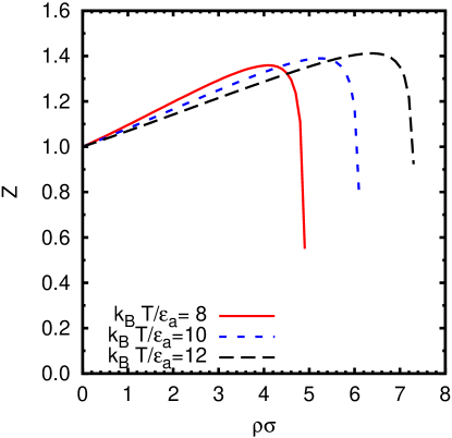
Figure 1 depicts the results of the virial —and hence energy, as remarked— route under the condition $\epsilon_{r}/\epsilon_{a}=2$, which constitutes the borderline range of stability of the one-dimensional PSW model with $\Delta/\sigma<1$.Santos08 Under this demanding condition, we have considered three reduced temperatures from $k_{B}T/\epsilon_{a}=8$ to $k_{B}T/\epsilon_{a}=12$, whereas the width of the well has been fixed to the value $\Delta/\sigma=1$. We remark that $\rho\sigma$ is not limited in values from above due to the boundness of the potential. The clear downturn of all three curves for sufficiently large reduced density $\rho\sigma$ is a consequence of the existence of a maximum density $\rho_{\max}$ [see Eq. (52)], beyond which the HPA breaks down, as described at the end of Appendix B. In particular, the values of the maximum density for $\epsilon_{r}/\epsilon_{a}=2$ and $\Delta/\sigma=1$ are $\rho_{\max}\sigma=4.94$, $6.15$, and $7.36$ at $k_{B}T/\epsilon_{a}=8$, $10$, and $12$, respectively, in agreement with Fig. 1.

Figure 2: Comparison between the compressibility factor $Z=\beta p/\sigma$ from the virial(-energy) and the compressibility route to the pressure. The circles represent MC simulation results. Chosen parameters are $\epsilon_{r}/\epsilon_{a}=2$, $\Delta/\sigma=1$, and $k_{B}T/\epsilon_{a}=10$.

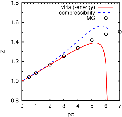
We compare in Fig. 2 the results from the virial(-energy) and the compressibility routes with MC simulationsnote1 for an intermediate value of the reduced temperature ($k_{B}T/\epsilon_{a}=10$) and other parameters as before. Rather interestingly, the virial(-energy) route appears to reproduce rather well the numerical simulation results up to the region where the artificial downward behavior shows up, whereas the compressibility route begins to deviate for densities $\rho\sigma>3$.

Figure 3: Rough estimate of the region of reliability for the HPA, on the basis of the consistency between the virial(-energy) and compressibility routes, in the reduced density $\rho\sigma$ versus reduced temperature $k_{B}T/\epsilon_{a}$ plane. Here the curves (a)–(d) correspond to $(\epsilon_{r}/\epsilon_{a},\Delta/\sigma)=(5,0.5)$, $(5,1)$, $(2,1)$, and $(2,0.5)$, respectively. The region below each curve represents states where the relative deviation between the virial(-energy) route and the compressibility one is smaller than $5\%$ and hence regarded as reliable. The inset shows the curves in the $\rho\sigma$ versus $k_{B}T/\epsilon_{r}$ plane for $(\epsilon_{r}/\epsilon_{a},\Delta/\sigma)=(2,1)$ (dashed line) and $(5,1)$ (solid line).

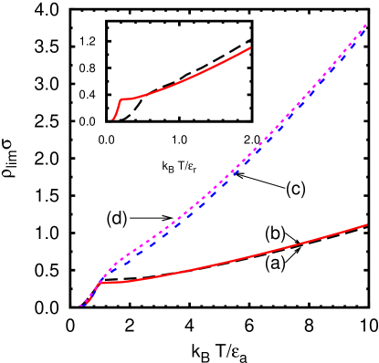
As the temperature increases the HPA theory clearly remains a good approximation for a larger range of densities. We can naturally measure this by the requirement that virial(-energy) and compressibility routes are consistent within a few percent. This is indeed shown in Fig. 3, where we depict a transition line separating a “reliable” from an “unreliable” regime, as measured by the relative deviation of the two routes (here taken to be $5\%$), for four choices of the model parameters: $(\epsilon_{r}/\epsilon_{a},\Delta/\sigma)=(2,1)$, $(2,0.5)$, $(5,1)$, and $(5,0.5)$. The value $\Delta/\sigma=0.5$ is frequently used in the SW counterpart.Vega95 We observe that the region $0\leq\rho\leq\rho_{\text{lim}}(T)$ where the HPA is reliable is hardly dependent on $\Delta/\sigma$ [compare curves (a)&(b) and (c)&(d) in Fig. 3]. On the other hand, at given values of $\Delta/\sigma$ and $k_{B}T/\epsilon_{a}$, the range $0\leq\rho\leq\rho_{\text{lim}}(T)$ decreases with increasing $\epsilon_{r}/\epsilon_{a}$ [compare curves (a)&(d) and (b)&(c) in Fig. 3], as expected. However, this effect is much less important if the increase of $\epsilon_{r}/\epsilon_{a}$ takes place at fixed $k_{B}T/\epsilon_{r}$ (see inset of Fig. 3). It is interesting to note that, as illustrated by Fig. 2, the HPA virial route keeps being reliable up to a certain density higher than $\rho_{\text{lim}}$.

Figure 4: Regions of reliability for the LPA and the HPA in the reduced density $\rho\sigma$ versus reduced temperature $k_{B}T/\epsilon_{a}$ plane. Here $\epsilon_{r}/\epsilon_{a}$=5 and $\Delta/\sigma=1$. The labels LPA, HPA, and LPA+HPA indicate the regions where only the LPA, only the HPA, or both approximations are reliable, respectively.

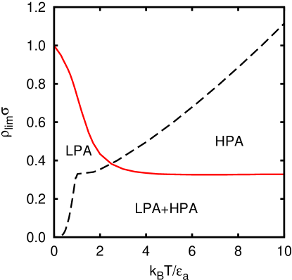
As said above, in Ref. Fantoni09, we introduced a LPA that was accurate for states where the penetrability effects were low or moderate. The LPA is complemented by the HPA presented in this paper. It is then interesting to compare the regions where each approximation can be considered reliable according to the same criterion as in Fig. 3. This is shown in Fig.  4 for the case $\epsilon_{r}/\epsilon_{a}=5$ and $\Delta/\sigma=1$. The two transition lines split the plane into four regions: a region where only the LPA is reliable, a region where only the HPA is reliable, a region where both approximations are reliable (and provide equivalent results), and a region where none of them is sufficiently good. The latter region shrinks as $\epsilon_{r}/\epsilon_{a}$ decreases (thanks to the HPA) or $\Delta/\sigma$ decreases (thanks to the LPA).

VI Structure

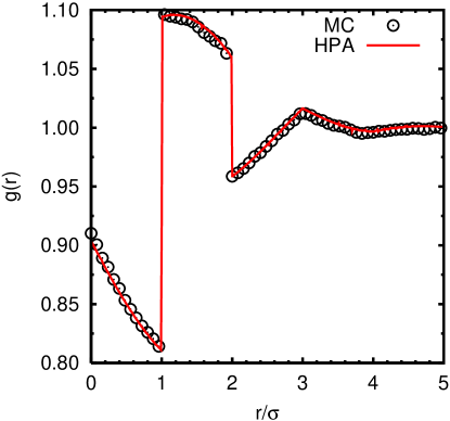
As an additional test of the soundness of the HPA, we also study the RDF $g(r)=h(r)+1$, which can easily be obtained from Eqs. (11) and (12), or equivalently from Eq. (16), once the auxiliary function $w(r)$ has been determined. For a sufficiently high temperature (and hence high penetrability), the HPA is clearly well performing, as can be inferred from Fig. 5, when compared with standard NVT MC results. Here we have considered the same parameters as in the preceding section ($\epsilon_{r}/\epsilon_{a}=2$ and $\Delta/\sigma=1$) at a corresponding high-temperature value $k_{B}T/\epsilon_{a}=10$ and a density $\rho\sigma=1.5$ where overlappings are unavoidable. Under these conditions, there is no visible difference among the various approximations considered in Section IV. The excellent performance of the HPA observed in Fig. 5 agrees with the reliability criterion of Fig. 3 since the state $k_{B}T/\epsilon_{a}=10$ and $\rho\sigma=1.5$ is well below the curve (c) corresponding to $\epsilon_{r}/\epsilon_{a}=2$ and $\Delta/\sigma=1$.

Figure 5: Results for the RDF $g(r)$ as a function of $r/\sigma$ with $\epsilon_{r}/\epsilon_{a}=2$, $\Delta/\sigma=1$, $k_{B}T/\epsilon_{a}=10$, and $\rho\sigma=1.5$. Predictions from the HPA (solid line) are compared with MC results (circles).

Figure 6: Comparison of different approximations in the results for the RDF $g(r)$ vs $r/\sigma$. Chosen parameters are $\epsilon_{r}/\epsilon_{a}=2$, $\Delta/\sigma=1$, and $\rho\sigma=1.5$. MC results (circles) are compared with the HPA (solid line), the nlHPA (dashed line), the mHPA (short dashed line), and the MSA (long dashed line). The two different panels refer to different reduced temperatures: $k_{B}T/\epsilon_{a}=5$ (top panel) and $k_{B}T/\epsilon_{a}=3$ (bottom panel). Note that both panels are drawn within the same scale.

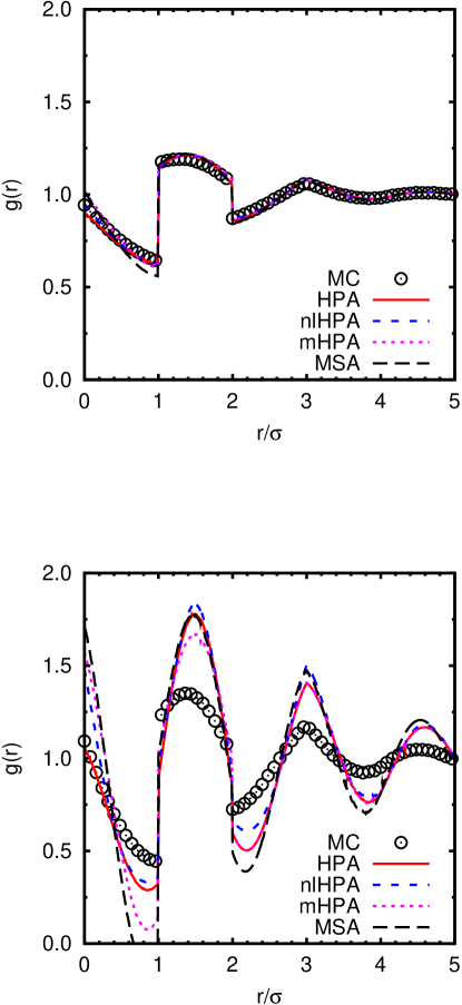
As we cool down, significant differences among various approximations (HPA, nlHPA, mHPA, and MSA) begin to appear, as depicted in Fig. 6, where results corresponding to temperatures $k_{B}T/\epsilon_{a}=5$ (top panel) and $k_{B}T/\epsilon_{a}=3$ (bottom panel) are reported within the same scale. The state $k_{B}T/\epsilon_{a}=5$ and $\rho\sigma=1.5$ is still lying in the reliable region of Fig. 3, but close to the boundary line (c), while the state $k_{B}T/\epsilon_{a}=3$ and $\rho\sigma=1.5$ is clearly outside that region. In the case $k_{B}T/\epsilon_{a}=5$ the HPA and its three variants are practically indistinguishable, except in the region $0<r<\sigma$, which is very important to describe the correct thermodynamic behavior, where the best agreement with MC data corresponds to the nlHPA, followed by the HPA. The two approximations that do not preserve the continuity of the cavity functions (mHPA and MSA) overestimate the jump at $r=\sigma$. In the lower temperature case $k_{B}T/\epsilon_{a}=3$ all the approximations overestimate the oscillations of the RDF. Interestingly, the HPA captures quite well the values of $g(r)$ near the origin. The worst overall behavior corresponds again to the MSA, which even predicts negative values of $g(r)$ for $r/\sigma\lesssim 1$.

Figure 7: An additional comparison of different approximations in the results for the RDF $g(r)$ vs $r/\sigma$. Here fixed parameters are $\epsilon_{r}/\epsilon_{a}=5$ and $\Delta/\sigma=0.5$. MC results (circles) are compared with the HPA (solid line), the nlHPA (dashed line), the mHPA (short dashed line), and the MSA (long dashed line). The top panel refers to the state $k_{B}T/\epsilon_{a}=5$ and $\rho\sigma=1.5$, whereas the bottom panel refers to $k_{B}T/\epsilon_{a}=2$ and $\rho\sigma=0.8$. In the bottom panel the MSA is not depicted. Again both panels are on the same scale.

Figure 8: Comparison of different approximations in the results for the RDF $g(r)$ vs $r/\sigma$. Chosen parameters are $\epsilon_{r}/\epsilon_{a}=5$, $\Delta/\sigma=1$, $k_{B}T/\epsilon_{a}=2$, and $\rho\sigma=0.2$. MC results (circles) are compared with the HPA (solid line) and the LPA (dashed line).

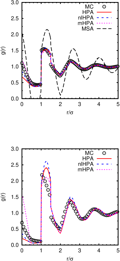
Additional insights can be obtained by decreasing the range of interactions, in close analogy with what we considered in previous work for the complementary LPA.Fantoni09 This is reported in Fig. 7 for the case $\epsilon_{r}/\epsilon_{a}=5$ and $\Delta/\sigma=0.5$ with $(k_{B}T/\epsilon_{a},\rho\sigma)=(5,1.5)$ (top panel) and $(k_{B}T/\epsilon_{a},\rho\sigma)=(2,0.8)$ (bottom panel). Again we stress that the same scale is used for both panels in order to emphasize the effect of lowering the temperature. Clearly this is a more demanding situation. In fact, both states are above curve (a) of Fig. 3 and thus outside the corresponding reliability region. Therefore, clear deviations from MC results appear in all considered approximations, especially in the lower temperature case $k_{B}T/\epsilon_{a}=2$ (bottom panel). Yet, the HPA is still a reasonably good approximation that follows the main qualitative features of the correct $g(r)$. In the higher temperature case $k_{B}T/\epsilon_{a}=5$ the only noticeable limitations of the HPA practically take place near the origin, this deficiency being largely corrected by the mHPA.

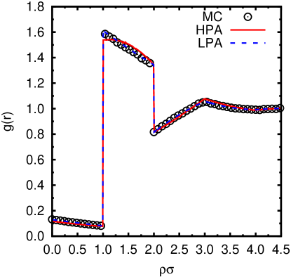
To conclude this section, it is worthwhile comparing the two complementary approaches HPA and LPA at a case where both are expected to be reliable, according to the diagram of Fig. 4. This is done in Fig. 8 for $\epsilon_{r}/\epsilon_{a}=5$, $\Delta/\sigma=1$, $k_{B}T/\epsilon_{a}=2$, and $\rho\sigma=0.2$. We observe that both approximations agree well each other and with MC data, except in the region $1<r/\sigma<\Delta/\sigma$, where the HPA RDF presents an artificial curvature.

VII Fisher–Widom line and fluid-fluid transition

We now turn to an interesting point raised in previous work,Fantoni09 namely the question of whether the model can display a phase transition in spite of its one-dimensional character.

The existence of general theorems —all essentially based on the original van Hove’s resultVanHove50 — on the absence of phase transitions for a large class of one-dimensional models with short-range interactions is well established.Cuesta04 PSW and PS models, however, do not belong to the class for which these general theorems hold. This is because boundness allows multiple partial (or even total) overlapping at some energy cost, thus rendering invalid the arguments used in the aforementioned theorems.

On the other hand, none of these theorems provide a general guideline to understand whether a one-dimensional model may or may not display a non-trivial phase transition, and one has then to rely on the specificity of each model.

As discussed in our previous work,Fantoni09 it is instructive to first address the simpler question of the location of the Fisher–Widom (FW) line. This is a line separating two different regimes for the large-distance behavior of the RDF $g(r)$ in the presence of competing repulsive/attractive interactions.Fisher69 The rationale behind the FW line is that on approaching the critical points where attractions become more and more effective, the behavior of correlation functions must switch from oscillatory (characteristic of repulsive interactions) to exponential with a well defined correlation length $\xi$. In the previous work, we analyzed the location of this line for PSW within the LPA. Here we extend this analysis to the HPA regime and discuss the compatibility of the two results.

Let us first briefly recall the main points of the analysis, referring to Ref. Fantoni09, for details. From Eq. (11) we note that the asymptotic behavior of $g(r)$ is the same as that of $y(r)$. In view of Eq. (12), this is hence related to $w(r)$, whose asymptotic behavior is governed by the pair of conjugate poles of $\widetilde{w}(k)$ with an imaginary part closest to the origin. If the real part of the pair is zero, the decay is monotonic and oscillatory otherwise.

According to Eq. (13), the poles of $\widetilde{w}(k)$ are given by

$$\rho\gamma_{r}\widetilde{f}_{\text{SW}}\left(k\right) = 1.$$ (30)

Let $k=\pm ix$ be the imaginary pole and $k=\pm i(x^{\prime}\pm iy)$ be the pole with the imaginary part closest to the origin. The FW line is determined by the condition $x=x^{\prime}$. This gives, at a given temperature, three equations in the three unknowns $x$, $y$, and $\rho$.Fantoni09 More specifically, after some algebra, one gets

$$\frac{y}{x}\sinh x \sinh(\lambda x) \left[\cos y-\cos(\lambda y)\right]=\sinh x\cosh(\lambda x)$$ (31)

$$\times\sin(\lambda y)(\cos y-1)-\sinh(\lambda x)\cosh x$$

$$\times\sin y\left[\cos(\lambda y)-1\right],$$

$$\gamma=\left[\frac{\sinh(\lambda x)}{\sinh x}\frac{\cos(\lambda y)-1}{\cos y-1}-1\right]^{-1},$$ (32)

$$\rho=\frac{1}{2\gamma_{r}}\frac{x}{\gamma\sinh(\lambda x)-(1+\gamma)\sinh x}.$$ (33)

The inverse of the parameter $x$ represents the correlation length $\xi=1/x$. From a practical point of view it is more convenient to use $x$ rather than $k_{B}T/\epsilon_{a}$ as a free parameter to construct the FW line. In that way, Eq. (31) becomes a transcendental equation that gives $y$ as a function of $x$; once $y(x)$ is known, the solution to Eq. (32) gives $k_{B}T/\epsilon_{a}$ as a function of $x$; finally, insertion of $y(x)$ and $k_{B}T(x)/\epsilon_{a}$ into Eq. (33) provides $\rho(x)$. The corresponding values of the pressure are obtained from either Eq. (25) (virial-energy route) or Eq. (26) (compressibility route).

We observe that $T$ decreases as $x$ decreases, until a critical value $T_{c}$ is found in the limit $x\to 0$. In that limit, Eqs. (31)–(33) simplify to

$$\lambda{y_{c}}\left[\cos y_{c}-\cos(\lambda y_{c})\right] = \sin(\lambda y_{c})(\cos y_{c}-1)-\lambda\sin y_{c}$$ (34)

$$\times\left[\cos(\lambda y_{c})-1\right],$$

$$\gamma_{c}=\left[\lambda\frac{\cos(\lambda y_{c})-1}{\cos y_{c}-1}-1\right]^{-1},$$ (35)

$$\rho_{c}=\frac{1}{2\gamma_{r}}\frac{1}{\gamma_{c}\Delta-1}.$$ (36)

At the critical point $T=T_{c}$ and $\rho=\rho_{c}$, one has $x=0$ or, equivalently, $\xi\to\infty$. Therefore, at this point $w(r)$ does not decay for long distances and in Fourier space one has $\widetilde{w}(k)\sim k^{-2}$ and $S(k)\sim k^{-2}$ for short wave numbers. The condition $S(k)\sim k^{-2}$ is also satisfied for $T<T_{c}$ if $\rho\sigma=\left[2\gamma_{r}(\gamma\Delta/\sigma-1)\right]^{-1}$, in agreement with Eq. (19). This defines in the $\rho$-$T$ plane a spinodal line or locus of points of infinite isothermal compressibility (within the compressibility route). The spinodal line cannot be extended to temperatures larger than the critical value $T_{c}$ because $\left[2\gamma_{r}(\gamma\Delta/\sigma-1)\right]^{-1}\geq\rho_{\max}\sigma$ if $T\geq T_{c}$, where $\rho_{\max}$ is the maximum density beyond which the HPA is unphysical at a given temperature (see Appendix B). We further note that the spinodal line only has a lower density (or vapor-like) branch, thus hampering the interpretation of $(T_{c},\rho_{c})$ as a conventional critical point.

The above features are already suggestive of considering the HPA spinodal line as an artifact of the theory when used in a region of parameter space where the approximation is invalid. Additional support to this view stems from the fact that the HPA keeps predicting a spinodal line and a critical point even in the SW case ($\epsilon_{r}/\epsilon_{a}\to\infty$, $\gamma_{r}\to 1$), a clearly incorrect feature. As we shall discuss further below, specialized numerical simulations coupled with a recent analytical study,Fantoni10 strongly support the absence of any phase transition in the present one-dimensional PSW model.

Figure 9: Plot of the FW transition line in the $\rho\sigma$ vs $k_{B}T/\epsilon_{a}$ plane with $\Delta/\sigma=1$ and $\epsilon_{r}/\epsilon_{a}=10$ (top panel) and $\epsilon_{r}/\epsilon_{a}=5$ (bottom panel). The long dashed curves are the spinodal lines predicted by the HPA. The FW and spinodal liness meet at the critical point (denoted by a circle).

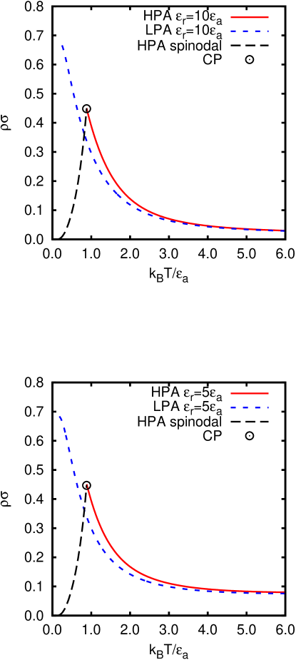
In Fig. 9 we report the comparison between the FW lines, as predicted by the LPA and the HPA, in the $\rho\sigma$ vs $k_{B}T/\epsilon_{a}$ plane for $\Delta/\sigma=1$ and two different energy ratios $\epsilon_{r}/\epsilon_{a}=10$ and $\epsilon_{r}/\epsilon_{a}=5$. The spinodal line predicted by the HPA is also included. As said above, the FW and spinodal lines meet at the critical point. While at high temperatures (above $k_{B}T/\epsilon_{a}=3$) there is a remarkable agreement between the two approximations, deviations occur at lower temperatures.

Figure 10: Same as in Fig. 9, but in the $p\sigma/\epsilon_{a}$ vs $k_{B}T/\epsilon_{a}$ plane. Note that while in the LPA the three routes to the pressure are not distinguishable one from the other on the graph scale, for the HPA the difference between the virial and the compressibility route is noticeable at low temperatures.

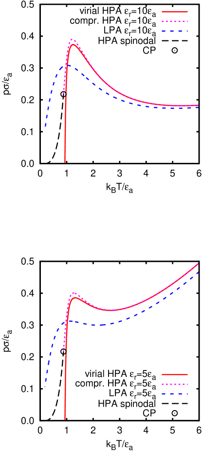
As in the original work by Fisher and Widom,Fisher69 we also report the FW line in the $p\sigma/\epsilon_{a}$ vs $k_{B}T/\epsilon_{a}$ plane (see Fig. 10), where again we compare the lines as derived from the HPA and LPA schemes. For the energy ratio $\epsilon_{r}/\epsilon_{a}=10$ (top panel) we see that the HPA and the LPA give qualitative similar forms of the FW line with a significant deviation at low temperatures, where again the HPA FW line is interrupted at $T=T_{c}$. Note that, while all three standard routes give practically identical results within the LPA, the virial(-energy) route in the HPA differs from the compressibility one at low temperatures (more than $5\%$ for $k_{B}T/\epsilon_{a}\lesssim 1.2$). For consistency, the HPA spinodal line is obtained via the compressibility route only. Similar features occur for the second lower value of the energy ratio, namely $\epsilon_{r}/\epsilon_{a}=5$ (bottom panel). Again, the LPA and HPA lines are qualitatively similar, the three routes in the LPA provide indistinguishable results, and the virial and energy routes in the HPA deviate more than $5\%$ for $k_{B}T/\epsilon_{a}\lesssim 1.2$. The main distinctive feature in this case $\epsilon_{r}/\epsilon_{a}=5$ is a marked upswing of the tail of the FW line, absent the previous case $\epsilon_{r}/\epsilon_{a}=10$. This means that, on increasing penetrability —that is, on decreasing $\epsilon_{r}/\epsilon_{a}$— the transition from oscillatory (above the line) to monotonic (below the line) behaviors occurs at a higher pressure and a higher density for a fixed temperature $k_{B}T/\epsilon_{a}$.

Despite the important differences in the steps followed to derive the LPA and the HPA, it is noteworthy that they agree in the qualitative shape of the FW lines (even though the HPA predicts a spurious spinodal line). It is then reasonable to expect that the true FW line should interpolate the LPA line at low temperatures with the HPA line at high temperatures.

Finally, we now tackle the issue of the existence of a phase transition for the PSW one-dimensional model. In view of the HPA results on the seemingly existence of a spinodal line (and hence of a critical point), we here consider the fluid-fluid transition. As we shall see, our numerics is compatible with the absence of such a transition, thus supporting the view that the above findings of a spinodal line is indeed a consequence of the application of the HPA to a regime where the theory is not valid.

As the FW line always anticipates the critical point, as remarked, we can then look for the existence of a fluid-fluid coexistence line in the region predicted by the interpolation of the LPA and HPA Fisher–Widom lines. We have carried out extensive simulations of the PSW fluid using Gibbs ensemble Monte Carlo techniques and employing all standard improvements suggested in the literature.Panagiotopoulos87 ; Panagiotopoulos88 ; Smit89a ; Smit89b In order to validate our code, we tested it against the case of the one-dimensional SW potential, where exact analytical predictions for all thermodynamic quantities are available.

We have used up to $1000$ particles and carefully scanned the temperature range $0.1<k_{B}T/\epsilon_{a}<2.0$ and the density range $0.1<\rho\sigma<6$, as suggested by the FW line (see Fig. 9). We have also considered different values of $\epsilon_{r}/\epsilon_{a}$ and $\Delta/\sigma$ for cases giving a significant overlapping probability. In all the cases we have not found any signature of a fluid-fluid phase separation.

Although the absence of a critical transition is always much more difficult to assess as opposed to its presence, the first scenario is consistent with more than one indication. The first indication stems from a lattice model counterpart of the one-dimensional PSW model. This is discussed in Appendix C, where the lattice version of the PSW model is constructed following standard manipulations with the result that no phase transitions are present for finite occupancy. An additional evidence supporting the absence of any fluid-fluid or freezing transition stems from the very recent exact analytical work alluded to earlier,Fantoni10 that, using the methodology presented in Ref. Kastner08, , concludes that no phase transitions are present for the PSW and PS models in one dimension.

Figure 11: Plot of the RDF $g(r)$ obtained from MC simulations for $\epsilon_{r}/\epsilon_{a}=2$, $\Delta/\sigma=1.5$, $k_{B}T/\epsilon_{a}=10$, and $\rho\sigma=6$ (top panel) and $\rho\sigma=8$ (bottom panel).

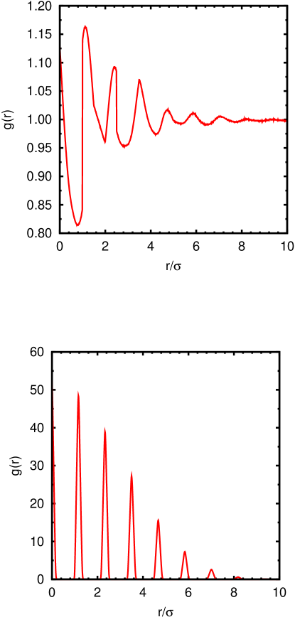
In our simulations we have also investigated values of $\epsilon_{r}/\epsilon_{a}$ and $\Delta/\sigma$ which violate Ruelle’s stability criterion (see Appendix A) and thus the one-dimensional PSW model is not necessarily stable in the thermodynamic limit. Here the phenomenology turns out to be much more interesting. For sufficiently low temperatures and sufficiently high densities we observe the formation of a “blob” of many-particle clusters (each made of a large number of overlapping particles) having a well defined and regular distribution on the axis, and occupying only a portion of the system length. In the “blob” phases the energy per particle grows with the number of particles, thus revealing the absence of a thermodynamic limit. The transition from a “normal” phase to a “blob” phase if $\epsilon_{r}/\epsilon_{a}<2(\ell+1)$, where $\ell$ is the integer part of $\Delta/\sigma$, is illustrated in Fig. 11. This figure shows the RDF at $\rho\sigma=6$ (top panel) and $\rho\sigma=8$ (bottom panel) for $\epsilon_{r}/\epsilon_{a}=2$, $\Delta/\sigma=1.5$, and $k_{B}T/\epsilon_{a}=10$. At the lower density the structure of the PSW fluid is qualitatively not much different from that expected if $\epsilon_{r}/\epsilon_{a}>2(\ell+1)$ (compare, for instance, with Fig. 6). However, the structure at the higher density is reminiscent of that of a solid, except that the distribution of particles does not span the whole length (here $L=N/\rho=62.5\sigma$). Instead, the particles distribute into a few clusters regularly spaced with distance $1.17\sigma$, so that the particles of a given cluster interact attractively with all the particles of the nearest- and next-nearest-neighbor clusters. Note that the number of particles within any given cluster is not necessarily identical. It is also worth noticing that, in spite of the huge difference in the vertical scales of both panels in Fig. 11, they are consistent with the condition $\int_{0}^{L/2}dr\,h(r)=-1/2\rho$.

The decay of the peaks of $g(r)$ is mainly due to the lack of translational invariance, i.e., the first and last clusters have only one nearest-neighbor cluster, the first, second, next-to-last, and last clusters have only one next-nearest-neighbor cluster, and so on.

We stress that the above phenomenon is specific of bounded potentials, such as PSW, and has no counterpart in the hard-core domain. It is then plausible to expect their appearance even in the corresponding three-dimensional versions of these models where freezing transition (and phase separation for SW) are present but could both be hampered by the presence of this clustering phenomenon in the region of parameter space where Ruelle’s stability criterion is violated. This would extend the interesting phenomenology already established for the PS case Likos01b . Work along these lines on the three-dimensional case is underway and will be reported elsewhere.

VIII Conclusions

In this paper we have completed the study initiated in previous workSantos08 ; Fantoni09 on the penetrable-square-well model in one-dimension. This is a model combining the three main ingredients present in many colloidal-polymer solutions, namely repulsions, attractions, and penetrability. While the first two are ubiquitous even in simple fluids, the latter is a peculiarity of complex fluids where there exist many examples of colloid-polymer systems which are penetrable (with some energy cost) to some extent, and they involve both steric repulsions and short-range attractions. This model then captures all these crucial features at the simplest level of description within an implicit solvent description.

The main new point of this paper was to present an additional and complementary approximation, denoted as the HPA, valid in regimes complementary to those valid for the low-penetrability scheme LPA discussed in Ref. Fantoni09, . While the idea behind the LPA was to modify the exact relations valid for the one-dimensional SW fluid —and in fact for any fluid with a hard core and short-range attraction— to allow penetrability within some reasonable approximation, the driving force behind the HPA is the fact that for bounded potential the Mayer function can be made arbitrarily small by considering sufficiently high temperatures. As a consequence, only the linear chain diagrams need to be retained at each order in the cluster expansion. As it turns out,Santos09 this is tantamount to considering the celebrated Debye–Hückel theory for charged fluids, and we have here considered the soundness of this approximations at various regimes as compared to specialized MC simulations. The latter were also compared with other approximations which parallel the entire hierarchy of approximations in the framework of charged fluids, ranging from the most sophisticated non-linear Debye–Hückel to the simplest mean-spherical approximations. We have assessed the regime of reliability of these approximations both for thermodynamic and correlation functions by comparison with MC simulations and by internal consistency between different routes to thermodynamics.

Next we have also discussed the location of the FW line, separating oscillatory from monotonic behavior in the correlation function, within the HPA and compared with that obtained from the LPA introduced in previous work.Fantoni09 In agreement with previous findings, we find that penetrability enhances the region where correlation functions have a monotonic regime. The FW derived from the HPA and LPA schemes are found to be in qualitative agreement thus making it possible the drawing of a line interpolating the high- and low-temperature regimes.

As a final point, we investigated the possibility of a fluid-fluid transition. This possibility arises because the boundness of the potential renders the van Hove theorem on the absence of phase transition for one-dimensional model with short-range interactions non-applicable. In fact, the HPA is seen to predict a critical point where the FW line meets a spinodal line. However, this prediction takes place in a region of densities and temperatures where the HPA is not reliable. A careful investigation using both NVT and Gibbs ensemble Monte Carlo techniques akin to those exploited in the investigations of the analog problem for the three-dimensional SW model yields negative results. These findings are also supported by analytical arguments based on the lattice gas counterpart where the absence of transition can be motivated by the absence of an infinite occupancy of each site, as well as by an exact analytical proofFantoni10 of a no-go theorem proving the absence of any phase transition in this model, which is in agreement with, and beautifully complements, our work.

In our quest for a possible thermodynamic transition in the one-dimensional PSW model we have explored values of the energy ratio $\epsilon_{r}/\epsilon_{a}$ and well width $\Delta/\sigma$ for which the stability of the system in the thermodynamic limit is not guaranteed by Ruelle’s criterion.Fisher66 ; Ruelle69 We have found that, as the temperature decreases and/or the density increases, a transition from a normal fluid phase to a peculiar solid-like phase takes place. The latter phase is characterized by the formation of clusters of overlapping particles occupying a small fraction of the available space and with non-extensive properties. This clustering transition preempts both the fluid-fluid and fluid-solid transitions.

In view of the results presented here, it would be very interesting to discuss the phase diagram of the corresponding three-dimensional PSW model. The phase diagram of the SW model ($\epsilon_{r}/\epsilon_{a}\to\infty$) is indeed well established and includes both a fluid-solid transition —present even in the HS counterpart— and a fluid-fluid transition line. The latter is present for any value of $\epsilon_{a}$ and $\Delta/\sigma$ but is stable against freezing only for $\Delta/\sigma>0.25$, the depth of the well being irrelevant. Kranendonk88 The results presented here strongly suggest the importance of the additional parameter $\epsilon_{r}/\epsilon_{a}$. A first interesting issue would be the Ruelle instability in three-dimensions. A straightforward extension of the arguments presented in Appendix A predicts a guaranteed stability for $\epsilon_{r}/\epsilon_{a}>12$ (if $\Delta/\sigma<1$), but the actual onset of the instability cannot be assessed through these arguments. One could expect that for sufficiently high penetrability (i.e., $\epsilon_{r}/\epsilon_{a}<12$ and high density) a phenomenon akin to the “clustering” transition found here could be present. In the case $\epsilon_{r}/\epsilon_{a}>12$, where the clustering transition is not expected, the interesting point is to assess the influence of the ratio $\epsilon_{r}/\epsilon_{a}$ on the location of the fluid-fluid critical point and coexistence line. All of this opens the possibility of a rich and interesting phase diagram which would complement that already present in a general class of bounded potentials with no attractive tails. Likos01b ; Likos07 We note that the high-penetrability regime is indeed the realm of the HPA presented here, which can be obviously extended to three-dimensions.

Work on the three-dimensional PSW model including the above points and other aspects is underway and will be reported elsewhere.

Appendix A Ruelle’s stability criterion

Let us consider the 1D PSW model characterized by $\epsilon_{r}/\epsilon_{a}$ and $\Delta/\sigma$. Let us call $\ell$ the integer part of $\Delta/\sigma$, i.e., $\ell\leq\Delta/\sigma<\ell+1$. According to Ruelle’s criterion, a sufficient condition of thermodynamic stability is Fisher66 ; Ruelle69

$$U_{N}(x_{1},\ldots,x_{N})=\sum_{i=1}^{N-1}\sum_{j=i+1}^{N}\phi(|x_{i}-x_{j}|)\geq-NB$$ (37)

for all configurations $\{x_{i}\}$, where $B$ is a fixed bound.

Given the number of particles $N$, we want to obtain the configuration with the minimum potential energy $U_{N}$. Without loss of generality we can see any given configuration as a set of $M$ clusters $(1\leq M\leq N)$, each cluster $i$ being made of $s_{i}$ overlapping particles (i.e., any pair of particles of a given cluster are separated a distance smaller than $\sigma$). In Ref. Santos08, we proved that for a fixed value of $M$ the minimum energy corresponds to $s_{i}=s=N/M$, all the particles of each cluster being located at the same point and the centers of two adjacent clusters being separated a distance $\sigma$. Therefore, we can restrict ourselves to this class of ordered configurations and use $s$ as the variational variable.

The repulsive contribution to the potential energy is

$$U_{N}^{r}(s)=M\frac{s(s-1)}{2}\epsilon_{r}.$$ (38)

To compute the attractive contribution we need to take into account that all the particles of a given cluster interact attractively with the particles of the $\ell+1$ nearest clusters. The total number of pairs of interacting clusters are $(\ell+1)[M-(\ell+1)]+\ell+(\ell-1)+(\ell-2)+\cdots+1=(\ell+1)\left(M-1-\ell/2\right)$. Therefore,

$$U_{N}^{a}(s)=-(\ell+1)\left(M-\frac{\ell+2}{2}\right)s^{2}\epsilon_{a}.$$ (39)

The total potential energy $U_{N}=U_{N}^{r}+U_{N}^{a}$ is

$$U_{N}(s)=N\frac{s-1}{2}\epsilon_{r}-(\ell+1)\left(N-\frac{\ell+2}{2}s\right)s\epsilon_{a}.$$ (40)

We then see that the value that minimizes $U_{N}(s)$ is

$$s_{*}=\frac{N}{\ell+2}\left[1-\frac{\epsilon_{r}}{2(\ell+1)\epsilon_{a}}\right].$$ (41)

This value is only meaningful if ${\epsilon_{r}}/{2(\ell+1)\epsilon_{a}}<1$. Otherwise, $s_{*}=1$. In summary, the absolute minimum value of $U_{N}$ is

$$U_{N}^{*}=U_{N}(s_{*})=\begin{cases}-\frac{N}{2}\left\{\epsilon_{r}+N\frac{\ell+1}{\ell+2}\epsilon_{a}\left[1-\frac{\epsilon_{r}}{2(\ell+1)\epsilon_{a}}\right]^{2}\right\},&{\epsilon_{r}}<{2(\ell+1)\epsilon_{a}},\\ -(\ell+1)\left(N-\frac{\ell+2}{2}\right)\epsilon_{a},&\epsilon_{r}>2(\ell+1)\epsilon_{a}.\end{cases}$$ (42)

Therefore, if ${\epsilon_{r}}>{2(\ell+1)\epsilon_{a}}$ the potential energy is bounded from below by $-NB$ with $B=(\ell+1)\epsilon_{a}$ and thus the system is stable in the thermodynamic limit. On the other hand, if ${\epsilon_{r}}<{2(\ell+1)\epsilon_{a}}$ there exist configurations that violates Ruelle’s criterion and so the thermodynamic stability of the system is not guaranteed.

Appendix B Density expansion of $w(r)$ within the HPA

Starting from Eq. (13) and for $\rho\gamma_{r}|\widetilde{f}_{\text{SW}}(k)|<1$, the Fourier transform $\widetilde{w}(k)$ can be expanded in power series as

$$\widetilde{w}\left(k\right) = \sum_{n=2}^{\infty}\left(\rho\gamma_{r}\right)^{n-1}\widetilde{f}_{\text{SW}}^{n}\left(k\right)~{}.$$ (43)

Upon inverse Fourier transform one then has

$$w\left(r\right) = \sum_{n=2}^{\infty}\left(\rho\gamma_{r}\right)^{n-1}w_{n}\left(r\right)~{},$$ (44)

where

$$w_{n}\left(r\right) = \int_{-\infty}^{\infty}\frac{dk}{2\pi}e^{ikr}\widetilde{f}_{\text{SW}}^{n}\left(k\right)~{}.$$ (45)

Equation (14) can be rewritten as

$$\widetilde{f}_{\text{SW}}(k)=\frac{i}{k}\left[(1+\gamma)\left(e^{ik}-e^{-ik}\right)-\gamma\left(e^{ik\lambda}-e^{-ik\lambda}\right)\right].$$ (46)

Therefore,

$$\widetilde{f}_{\text{SW}}^{n}\left(k\right) = \frac{i^{n}}{k^{n}}\sum_{m=0}^{n}\sum_{p=0}^{m}\sum_{q=0}^{n-m}\binom{n}{m}\binom{m}{p}\binom{n-m}{q}$$

$$\times(-1)^{m+p+q}\left(1+\gamma\right)^{m}\gamma^{n-m}$$

$$\times{e^{ik[2p-m+(2q-n+m)\lambda]}}~{}.$$ (47)

The origin ($k=0$) is a regular point of $\widetilde{f}_{\text{SW}}(k)$ and hence of $\widetilde{f}_{\text{SW}}^{n}(k)$ [but not of each separate term in Eq. (47)], so we can choose to save the point $k=0$ in Eq. (45) either from above or from below. Here we do it from above with the result

$$\lim_{\epsilon\to 0^{+}}i^{n}\int_{\cal L}\frac{dk}{2\pi}\frac{e^{ikr}}{(k+i\epsilon)^{n}}=\frac{(-r)^{n-1}}{\left(n-1\right)!}\Theta\left(-r\right),\quad n>0,$$ (48)

where the path ${\cal L}$ in the complex $k$ plane goes from $k=-\infty$ to $k=+\infty$ and closes itself on the upper plane if $r>0$ and in the lower one if $r<0$. In Eq. (45) we then find

$$w_{n}(r) = \sum_{m=0}^{n}\sum_{p=0}^{m}\sum_{q=0}^{n-m}\binom{n}{m}\binom{m}{p}\binom{n-m}{q}(-1)^{m+p+q}\left(1+\gamma\right)^{m}\gamma^{n-m}$$ (49)

$$\times\frac{\left[-r-2p+m-\left(2q-n+m\right)\lambda\right]^{n-1}}{\left(n-1\right)!}\Theta\left[-r-2p+m-\left(2q-n+m\right)\lambda\right]~{}.$$

It is interesting to note that $w_{n}(r)=0$ if $r>\lambda n$. Thus Eq. (44) can be rewritten as

$$w(r) = \sum_{n=\max\{2,\left[r/\lambda\right]\}}^{\infty}\left(\rho\gamma_{r}\right)^{n-1}w_{n}\left(r\right)~{},$$ (50)

where $[r/\lambda]$ is the integer part of $r/\lambda$.

Figure 12: Plot of the radius of convergence $\gamma_{r}\rho_{\text{conv}}\sigma$ and of the maximum density $\gamma_{r}\rho_{\text{max}}\sigma$ versus $\gamma\Delta/\sigma$ for $\Delta/\sigma=0.5$ and $\Delta/\sigma=1$.

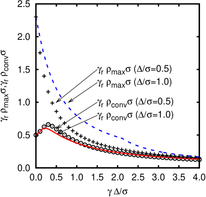
The radius of convergence of the series (50) depends on temperature and can be obtained by the same arguments as in the PS case.Malijevsky06 From the denominator of Eq. (13), it follows that the series converges provided that $\rho<\rho_{\text{conv}}$, where

$$(\gamma_{r}\rho_{\text{conv}})^{-1} = {\left|\widetilde{f}_{\text{SW}}\right|_{\max}}~{}.$$ (51)

Here $\left|\widetilde{f}_{\text{SW}}\right|_{\max}$ denotes the absolute maximum value of $\left|\widetilde{f}_{\text{SW}}(k)\right|$. From Eq. (14) if $\gamma<(\lambda^{3}-1)^{-1}$ that maximum corresponds to $k=0$, i.e., $\left|\widetilde{f}_{\text{SW}}\right|_{\max}=-\widetilde{f}_{\text{SW}}(0)$, and so $\gamma_{r}\rho_{\text{conv}}=(1-\gamma\Delta)^{-1}/2$. On the other hand, if $\gamma>(\lambda^{3}-1)^{-1}$ the maximum value $\left|\widetilde{f}_{\text{SW}}\right|_{\max}$ takes place at $k\neq 0$ and so $\gamma_{r}\rho_{\text{conv}}$ must be obtained numerically. For sufficiently large values of $\gamma\Delta$ one has $\left|\widetilde{f}_{\text{SW}}\right|_{\max}=\widetilde{f}_{\text{SW}}(0)$, so that $\gamma_{r}\rho_{\text{conv}}=(\gamma\Delta-1)^{-1}/2$ and this coincides with the maximum physical density (see below). Figure 12 shows $\gamma_{r}\rho_{\text{conv}}$ as a function of $\gamma\Delta$ for two values of $\Delta/\sigma$. In the PS limit ($\gamma\Delta\to 0$) one has $\gamma_{r}\rho_{\text{conv}}=\frac{1}{2}$. As the strength of the attractive part of the potential (measured by the product $\gamma\Delta$) increases, the radius of convergence first grows, reaches a maximum, and then decays.

Except when $\gamma\Delta$ is so large that $\left|\widetilde{f}_{\text{SW}}\right|_{\max}=\widetilde{f}_{\text{SW}}(0)$, the maximum $\left|\widetilde{f}_{\text{SW}}\right|_{\max}$ corresponds to a negative value of $\widetilde{f}_{\text{SW}}(k)$ and so the singularity responsible for the radius of convergence is located on the negative real axis. Therefore, $w(r)$ is still well defined beyond the radius of convergence, i.e., for $\rho>\rho_{\text{conv}}$. On the other hand, analogously to the PS case,AS04 ; GK77 the HPA for the PSW fluid becomes unphysical, at a given temperature, for densities larger than a certain value $\rho_{\text{max}}$ given by the condition

$$(\gamma_{r}\rho_{\text{max}})^{-1} = \widetilde{f}_{\text{SW}}^{\max}~{},$$ (52)

where $\widetilde{f}_{\text{SW}}^{\max}$ is the absolute maximum value of $\widetilde{f}_{\text{SW}}(k)$. Since $\widetilde{f}_{\text{SW}}^{\max}\leq\left|\widetilde{f}_{\text{SW}}\right|_{\max}$, it is obvious that $\rho_{\max}\geq\rho_{\text{conv}}$. For sufficiently large values of $\gamma\Delta$ (actually, for temperatures below the critical value $T_{c}$ defined in Section VII) one has $\widetilde{f}_{\text{SW}}^{\max}=\widetilde{f}_{\text{SW}}(0)$, and so $\gamma_{r}\rho_{\text{max}}=(\gamma\Delta-1)^{-1}/2$. In that case, the line of maximum density becomes a spinodal line, as discussed in Section VII. Figure 12 also includes a plot of $\gamma_{r}\rho_{\text{max}}$ as a function of $\gamma\Delta$ for the same two values of $\Delta/\sigma$. Note the kink of the curve $\gamma_{r}\rho_{\text{max}}$ for $\Delta/\sigma=1$ at the critical point ($\gamma_{c}\Delta/\sigma\simeq 2.11$, $\gamma_{r}\rho_{c}\simeq 0.45$), so that $\gamma_{r}\rho_{\text{max}}=(\gamma\Delta-1)^{-1}/2$ (spinodal line) if $\gamma\Delta/\sigma>2.11$.

Appendix C The PSW lattice gas

Consider the PSW model in one dimension. The grand partition function is

$$\Xi\left(\mu,L,T\right) = \sum_{N=0}^{\infty}\frac{1}{N!}\left(\frac{e^{\beta\mu}}{\Lambda_{T}}\right)^{N}Z_{N}\left(L,T\right),$$ (53)

where $\Lambda_{T}$ is the thermal de Broglie’s wavelength and

$$Z_{N}\left(L,T\right)=\int_{L}dr_{1}\ldots dr_{N}\exp\left[-\beta\frac{1}{2}\sum_{i\neq j=1}^{N}\phi\left(\mathbf{r}_{i}-\mathbf{r}_{j}\right)\right].$$ (54)

We now discretize the length $L$ as a sum of $N_{c}\gg 1$ cells of size $a=L/N_{c}$ with occupancy $n_{\alpha}$, $\alpha=1,\ldots,N_{c}$. The value of $a$ is chosen in the interval $\sigma<a<\sigma+\Delta$, with $\Delta<\sigma$, so that two particles in the same cell are assumed to interact repulsively and two particles in adjacent cells are assumed to interact attractively. The integral can then approximated as $\int_{L}dr\approx aN_{c}$ and the configurational partition function $Z_{N}$ as

$$Z_{N}\left(L,T\right) \approx a^{N}\sum_{\{n_{\alpha}\}}\delta_{N,\sum_{\alpha}n_{\alpha}}\exp\left[-\beta\frac{1}{2}\sum_{\alpha\beta=1}^{N_{c}}\chi_{\alpha,\beta}\tilde{\phi}_{\alpha\beta}\right]$$ (55)

$$\times N!.$$

In Eq. (55) the $\delta$ function accounts for the constraint $N=\sum_{\alpha}n_{\alpha}$ and the factor $N!$ of the indistinguishability of the particles. Also we have introduced $\chi_{\alpha\beta}$ accounting for multi-interactions among cells and $\tilde{\phi}_{\alpha\beta}$ which is equal to $\epsilon_{r}$ if $\alpha=\beta$ and equal to $-\epsilon_{a}$ for nearest-neighboring (nn) cells. Noting that each particle in an $\alpha$-cell can either interact with $n_{\alpha}-1$ other particles within the same cell or with $n_{\beta}$ particles within a nn $\beta$-cell, we see that

$$\frac{1}{2}\sum_{\alpha,\beta=1}^{N_{c}}\chi_{\alpha\beta}\tilde{\phi}_{\alpha\beta}=-\epsilon_{a}\sum_{\langle\alpha,\beta\rangle}n_{\alpha}n_{\beta}+\frac{1}{2}\epsilon_{r}\sum_{\alpha}n_{\alpha}\left(n_{\alpha}-1\right).$$ (56)

Substituting into Eq. (53) we then find

$$\Xi\left(\mu,L,T\right) = \sum_{N=0}^{\infty}\left(\frac{a}{\Lambda_{T}}e^{\beta\mu}\right)^{N}\sum_{\{n_{\alpha}\}}\delta_{N,\sum_{\alpha}n_{\alpha}}\exp\left[-\beta\frac{1}{2}\sum_{\alpha,\beta}\chi_{\alpha\beta}\tilde{\phi}_{\alpha\beta}\right].$$ (57)

Because of the $\delta$, the two sums can be inverted and the sum over $N$ can be explicitly carried out thus obtaining

$$\Xi\left(\mu,L,T\right) = \sum_{\{n_{\alpha}\}}\exp\left[-\beta\left(-\epsilon_{a}\sum_{\langle\alpha\beta\rangle}n_{\alpha}n_{\beta}+\frac{1}{2}\epsilon_{r}\sum_{\alpha}n_{\alpha}\left(n_{\alpha}-1\right)-\tilde{\mu}\sum_{\alpha}n_{\alpha}\right)\right]$$ (58)

with $\tilde{\mu}=\mu+(1/\beta)\ln(a/\Lambda_{T})$.

Assume a finite length $L$ (and hence a finite number of cells $N_{c}$) with periodic boundary conditions. The above partition function can then be solved by standard transfer matrix techniques

$$\Xi\left(\mu,L,T\right) = \sum_{\{n_{1},\ldots n_{N_{c}}\}}\prod_{\alpha=1}^{N_{c}}A_{n_{\alpha}n_{\alpha+1}}=\operatorname{Tr}A^{N_{c}},$$ (59)

where we have introduced the matrix

$$A_{n_{\alpha}n_{\beta}} = \exp\left[-\beta\left(-\epsilon_{a}n_{\alpha}n_{\beta}+\frac{\epsilon_{r}}{4}\left(n_{\alpha}\left(n_{\alpha}-1\right)+n_{\beta}\left(n_{\beta}-1\right)\right)-\frac{\widetilde{\mu}}{2}\left(n_{\alpha}+n_{\beta}\right)\right)\right].$$ (60)

If $N_{c}$ is finite, one then has in the thermodynamic limit

$$\lim_{L\to\infty}\frac{1}{L}\log\Xi\left(\mu,L,T\right) = \frac{1}{a}\log\lambda_{0},$$ (61)

where $\lambda_{0}$ is the largest eigenvalue of the matrix. Clearly this is analytic and no phase transitions are possible for finite occupancy $N_{c}$.

References

- (1) C. Marquest and T. A. Witten, J. Phys. (Paris) 50, 1267 (1989).
- (2) C. N. Likos, Phys. Rep. 348, 267 (2001).
- (3) F. H. Stillinger, J. Chem. Phys. 65, 3968 (1976).
- (4) C. N. Likos, M. Watzalwek, and H. Löwen, Phys. Rev. E 58, 3135 (1998).
- (5) A. Santos, R. Fantoni, and A. Giacometti, Phys. Rev. E 77, 051206 (2008).
- (6) R. Fantoni, A. Giacometti, Al. Malijevský, and A. Santos, J. Chem. Phys. 131, 124106 (2009).
- (7) Al. Malijevský and A. Santos, J. Chem. Phys. 124, 074508 (2006).
- (8) Al. Malijevský, S. B. Yuste, and A. Santos, Phys. Rev. E 76, 021504 (2007).
- (9) J.-P. Hansen and I. R. McDonald Theory of Simple Liquids (Academic Press, Amsterdam, 2006).
- (10) A. Santos, R. Fantoni, and A. Giacometti, J. Chem. Phys. 131, 181105 (2009).
- (11) L. Van Hove, Physica (Amsterdam) 16, 137 (1950).
- (12) J. A. Cuesta and A. Sanchez, J. Stat. Phys. 115, 869 (2004).
- (13) A. Z. Panagiotopoulos, Mol. Phys. 61, 813 (1987).
- (14) A. Z. Panagiotopoulos, N. Quirke, M. Stapleton, and D. J. Tildesley, Mol. Phys. 63, 527 (1988).
- (15) B. Smit, Ph. De Smedt, and D. Frenkel, Mol. Phys. 68, 931 (1989).
- (16) B. Smit and D. Frenkel, Mol. Phys. 68, 951 (1989).
- (17) R. Fantoni and M. Kastner, unpublished (2010).
- (18) M. Kastner, Rev. Mod. Phys. 80, 167 (2008).
- (19) M. E. Fisher and B. Widom, J. Chem. Phys. 50, 3756 (1969).
- (20) L. Acedo and A. Santos, Phys. Lett. A 323, 427 (2004).
- (21) A. Santos, J. Chem. Phys. 126, 116101 (2007).
- (22) C. N. Likos, A. Lang, M. Watzlawek and H. Löwen, Phys. Rev. E 63, 031206 (2001)
- (23) C. N. Likos, B. M. Mladek, D. Gottwald and G. Kahl, J. Chem. Phys. 126, 224502 (2007).
- (24) MC results were obtained from a standard NVT ensemble calculation with periodic boundary conditions. We used particles and MC steps, which were checked to be sufficient for a good accuracy.
- (25) C. Vega, L. F. Rull, and S. Lago, Phys. Rev. E 51, 3146 (1995).
- (26) M.E. Fisher and D. Ruelle, J. Math. Phys. 7, 260 (1966).
- (27) D. Ruelle, Statistical Mechanics: Rigorous Results (Benjamin, London, 1969).
- (28) W. G. T. Kranendonk and D. Frenkel, Mol. Phys. 64, 403 (1988).
- (29) N. Grewe and W. Klein, J. Math. Phys. 18, 1729, 1735 (1977); W. Klein and N. Grewe, J. Chem. Phys. 72, 5456 (1980).