Two simple systems with cold atoms: quantum chaos tests and nonequilibrium dynamics

Abstract

This article is an attempt to provide a link between the quantum nonequilibrium dynamics of cold gases and fifty years of progress in the low-dimensional quantum chaos. We identify two atomic systems lying on the interface: two interacting atoms in a harmonic multimode waveguide and an interacting two-component Bose-Bose mixture in a double-well potential. In particular, we study the level spacing distribution, the wavefunction statistics, the eigenstate thermalization, and the ability to thermalize in a relaxation process as such.

1 Introduction

In this article, we identify two simple atomic system lying on the interface between the nonequilibrium dynamics of cold gases and low-dimensional quantum chaos. The system of two short-range-interacting atoms in a harmonic waveguide is compared to the well studied Šeba billiard [1]. A two-component interacting Bose-Bose mixture in a double-well potential provides a realization of a quantum particle moving on a four-dimensional surface of a tensor product of two spheres under a non-integrable perturbation.

The waveguide problem allows for an exact analytic solution, in spite of the absence of a complete set of integrals of motion. The double-well problem reduces to a numerical diagonalization of a small, a-few-hundred-by-a-few-hundred matrix, a few minute calculation on a moderate laptop.

To assess the degree of quantum chaos, we utilize two standard quantum-chaotic measures: level spacing statistics [2, 3] and the statistics of the values of the wavefunction in the coordinate representation [4, 5]. The former predicts that the spectra of quantum-chaotic systems have the statistical properties of the spectra of random matrices. The latter dictates the Gaussian statistics for the wavefunction.

From the point of view of the nonequilibrium dynamics, we study both the degree of the eigenstate thermalization and the actual thermalization in an expansion from a class of realistic initial states. The eigenstate thermalization [6, 7, 8, 9, 10] – the suppression of the eigenstate-by-eigenstate variance of quantum expectation values of simple observables – provides an ultimate upper bound for a possible deviation of the relaxed value of an observable from its thermodynamical expectation, for any initial state in principle. However, recently a new direction of research has emerged: quantum quench in many-body interacting systems [11, 12, 13, 14, 15, 16, 17, 18, 19, 20, 21]. In this class of problems, the initial state is inevitably decomposed into a large superposition of the eigenstates of the Hamiltonian governing the dynamics, and the discrepancy between the result of the relaxation and thermal values is expected to be diminished.

Note that a related comprehensive study of the relationship between the quantum chaos and thermalization for atoms in optical lattices has been performed in Ref. [22].

2 Two bosons in a circular, transversely harmonic multimode waveguide

In the case of the relative motion of two short-range-interacting atoms in a circular, transversely harmonic waveguide [23] , the full Hamiltonian

$$\hat{H}=\hat{H}_{WG}+\hat{V}_{FH}$$ (1)

can be split onto an integrable, “free motion” part and a non-integrable perturbation. The unperturbed Hamiltonian is given by the sum of the longitudinal and transverse kinetic energies and the transverse trapping energy $\hat{U}=\mu\omega_{\perp}^{2}\rho^{2}/2$,

$$\hat{H}_{WG}=-{\hbar^{2}\over 2\mu}{\partial^{2}\over\partial z^{2}}-{\hbar^{2}\over 2\mu}\Delta_{\rho}+\hat{U}-\hbar\omega_{\perp}\quad,$$ (2)

where $\omega_{\perp}$ is the transverse frequency, $\Delta_{\rho}$ is the transverse two-dimensional Laplacian, $\mu=m/2$ is the reduced mass, and $m$ is the atomic mass. We will assume periodic boundary conditions along $z$, with a period $L$. In what follows, we will restrict the Hilbert space to the states of zero $z$-component of the angular momentum and even under the $z\leftrightarrow-z$ reflection. Note that the zero-range interaction has no effect on the rest of the Hilbert space. The non-interacting eigenstates are products of the transverse two-dimensional zero-angular-momentum harmonic wavefunctions, labeled by the quantum number $n\geq 0$, and the symmetric plane waves $\cos(2\pi lz/L)$, $l\geq 0$. The unperturbed spectrum is therefore given by $E_{nl}=2\hbar\omega_{\perp}n+\hbar^{2}(2\pi l/L)^{2}/(2\mu)$

The interaction $\hat{V}_{FH}$ in (2) couples the transverse and longitudinal degrees of freedom. We assume the interaction to be of the Fermi-Huang type. It can be symbolically represented as a separable rank I perturbation [24]:

$$\hat{V}_{FH}=V|{\cal L}\rangle\langle{\cal R}|,$$ (3)

with the formfactors $|{\cal L}\rangle=\delta_{3}({\bi r})$ and $\langle{\cal R}|=\delta_{3}({\bi r})(\partial/\partial r)(r\,\cdot)$. Here, the interaction strength is $V=(2\pi\hbar^{2}a_{s}/\mu)$, where $a_{s}$ is the three-dimensional $s$-wave scattering length. The rigorous definition of the operator (3) reads

$$\langle\chi|\hat{V}_{FH}|\psi\rangle\equiv V\chi^{\star}({\bi r}={\bf 0})\lim_{r\to 0}\frac{\partial}{\partial r}(r\psi(r,\,\theta,\,\phi))\quad.$$ (4)

Following the the Refs. [24, 1], it can be shown that the operator (4) produces a member of a (parametrized by $V$) family of self-adjoint extensions of the “free motion” Hamiltonian (2).

Note that the model (1), with an unbounded along $z$ motion, was first used to derive the effective one-dimensional atom-atom interaction in a monomode atom guide [25]. It was further extended to the multimode regime in Ref. [26], where the intermode kinetic coefficients were derived. In this article, we consider a bound-motion analogue of the multimode guide of Ref. [26], suitable for a study of the relaxation dynamics and chaotic properties.

Even though the perturbation of the form (3) destroys the complete set of integrals of motion of the unperturbed system, the problem can be solved exactly. The solution for the full system can be obtained as follows. The action of the perturbation on each wavefunction produces the left formfactor $|{\cal L}\rangle$. As a result, any eigenstate $|\alpha\rangle$ of the perturbed system functionally coincides with the Green function of the unperturbed Hamiltonian taken at the energy of the eigenstate $E_{\alpha}$. The following eigenenergy equation then applies, along with an expression for the eigenstates:

$$\sum\limits_{\vec{n}}{\langle{\cal R}|\vec{n}\rangle\langle\vec{n}|{\cal L}\rangle\over E_{\alpha}-E_{\vec{n}}}=\frac{1}{V},\quad|\alpha\rangle\propto\sum\limits_{\vec{n}}{|\vec{n}\rangle\langle\vec{n}|{\cal L}\rangle\over E_{\alpha}-E_{\vec{n}}},$$ (5)

where $|\vec{n}\rangle$ stands for an eigenstate of the unperturbed system of energy $E_{\vec{n}}$. Similar expressions were obtained in Refs. [1, 27] for the case of the Šeba billiard and its generalizations. Solutions of this type, for the integrable case of a spherically symmetric harmonic confinement, are presented in Ref. [28].

Substituting the above non-interacting eigenstates and eigenenergies to the Eq. (5) and summing over $l$, one obtains the following expression for the interacting eigenstates:

$$\langle\rho,z|\alpha\rangle=C_{\alpha}\sum\limits^{\infty}_{n=0}{\cos\left(2\sqrt{\epsilon_{\alpha}-\lambda n}\zeta\right)\over\sqrt{\epsilon_{\alpha}-\lambda n}\sin\sqrt{\epsilon_{\alpha}-\lambda n}}e^{-\xi/2}L^{(0)}_{n}\!\left(\xi\right),$$ (6)

where the rescaled energy $\epsilon_{\alpha}$ is given by $\epsilon_{\alpha}\equiv\lambda E/\left(2\hbar\omega_{\perp}\right)$, $\lambda\equiv\left(L/a_{\perp}\right)^{2}$ is the aspect ratio, $\zeta\equiv z/L-1/2$,  $\xi\equiv\left(\rho/a_{\perp}\right)^{2}$,   $L^{(0)}_{n}(\xi)$ are the Legendre polynomials, and $a_{\perp}=\left(\hbar/\mu\omega_{\perp}\right)^{1/2}$ is the size of the transverse ground state. The normalization constant $C_{\alpha}$ is expressed as

$$C_{\alpha}={2\over a_{\perp}\sqrt{\pi L}}\biggl{[}\sum\limits^{\infty}_{n=0}\biggl{(}{\cot\sqrt{\epsilon_{\alpha}-\lambda n}\over\left(\epsilon_{\alpha}-\lambda n\right){}^{3/2}}+{1\over\left(\epsilon_{\alpha}-\lambda n\right)\sin^{2}\sqrt{\epsilon_{\alpha}-\lambda n}}\biggr{)}\biggr{]}^{-1/2}.$$ (7)

Extracting the regular part of the wavefunction (6) via the procedure given in Refs. [26, 29], we arrive at the following transcendental equation for the eigenenergies $\epsilon_{\alpha}$:

$$\sqrt{\lambda}\sum\limits^{\infty}_{n=0}{\cot\sqrt{\epsilon_{\alpha}-\lambda n}+i\over\sqrt{\epsilon_{\alpha}-\lambda n}}-\zeta\left({1\over 2},-{\epsilon_{\alpha}\over\lambda}\right)={a_{\perp}\over a_{s}}\quad,$$ (8)

where $\zeta\left(\nu,x\right)$ is the Hurwitz $\zeta$-function (see [29]). The summands in the sums Eqs. (6), (7), and (8) decay exponentially with $n$, leading to the fast converging series. Note that the imaginary parts of the two terms in the left hand side of the (8) cancel each other automatically. Similar solutions were obtained for two atoms with a zero-range interaction in a cylindrically-symmetric harmonic potential [30] (that system was analyzed numerically in Ref. [31]). Higher partial wave scatterers were analyzed in the Ref. [32].

At rational values of $\lambda/\pi^{2}$ the unperturbed energy spectrum shows degeneracies that are not fully lifted in the full [deduced from (8)] spectrum. To minimize the effect of the degeneracies, we, following Ref. [1], fix the length of the guide by $(L/a_{\perp})^{2}\equiv\lambda=2\phi_{gr}\pi^{7}\approx 9774$, where $\phi_{gr}=(1+\sqrt{5})/2$ is the golden ratio.

3 A two-component interacting Bose gas in two coupled potential wells

Next, we are going to consider a two-component Bose-Bose mixture trapped in a two-well potential.

The second-quantized Hamiltonian is

$$\hat{H}=\hat{H}_{0}+\hat{V}$$ (9)

$$\hat{H}_{0}=\frac{1}{2}\sum_{i=a,\,b}\sum_{j=a,\,b}\left(U_{ijL}\hat{c}^{\dagger}_{iL}\hat{c}^{\dagger}_{jL}\hat{c}_{iL}\hat{c}_{jL}+U_{ijR}\hat{c}^{\dagger}_{iR}\hat{c}^{\dagger}_{jR}\hat{c}_{iR}\hat{c}_{jR}\right)$$ (10)

$$\hat{V}=-2J\sum_{i=a,\,b}(\hat{c}^{\dagger}_{iL}\hat{c}_{iR}+\hat{c}^{\dagger}_{iR}\hat{c}_{iL})\quad,$$ (11)

where $\hat{c}^{\dagger}_{iL}$($\hat{c}^{\dagger}_{iR}$) is the creation operator for the atom of the $i$-th type in the left(right) well, $a$ and $b$ denote the two species, and the factor of $-2$ in the definition of $V$ is used to ensure the consistency with the conventional definition of the hopping constant in the theory of multi-well lattices with periodic boundary conditions.

We fix the coupling constants $U_{ijL(R)}$ to $U_{aaR}=0.3041\,U,\,U_{abR}=1.0410\,U,\,U_{bbR}=0.3684\,U,\,U_{aaL}=0.3085\,U,\,U_{abL}=1.4574\,U,\,U_{bbL}=0.4524\,U$, where $U$ is the overall coupling strength. The relative strengths of the interaction were chosen once and for all from a uniform random distribution between $0$ and $2$. The same set was used in all further numerical experiments.

The set of deviations of the number of atoms of a given type in the right well from the half of the total number of atoms of this type constitutes a convenient set of quantum numbers: $s_{a}\equiv N_{aR}-N_{a}/2,\,s_{b}\equiv N_{bR}-N_{b}/2$, where $\hat{N}_{aR}\equiv\hat{c}^{\dagger}_{aR}\hat{c}_{aR}$ and $\hat{N}_{bR}\equiv\hat{c}^{\dagger}_{bR}\hat{c}_{bR}$. The observable $\hat{s}_{a}$ has been chosen to be the principal observable of interest in the eigenstate thermalization and relaxation studies. Below, we fix the numbers of atoms to $N_{a}=N_{b}=N=20$.

Analogously to the one-specie case [33], the Hamiltonian (9) is integrable in both $J\gg U$ and $J\ll U$ limits.

In the $J\ll U$ limit, the eigenstates are represented by the Fock states (eigenstates of $\hat{H}_{0}$, see (10)) where number of bosons of each type in each well is fixed. For our choice of the coupling constants, the energy as a function of $(s_{a},\,s_{b})$ constitutes a hyperboloid. At low energies, the spectrum of $\hat{H}_{0}$ is dominated by the eigenstates where the atoms of different type are localized in the opposite wells: $(s_{a},\,s_{b})\approx(\pm N,\,\mp N)$. At high energies, the atoms prefer to localize in the same well: $(s_{a},\,s_{b})\approx(\pm N,\,\pm N)$.

In the opposite limit $J\gg U$, the good quantum numbers are given by the numbers of particles of each type in the even and odd (with respect to the wells) one-body states. In this limit, the mean-field Hamiltonian

$$\hat{H}_{\mbox{\scriptsize mf}} \equiv \hat{V}+\langle\hat{H}_{0}\rangle$$

$$= \hat{V}+\frac{N}{8}\left((N-2)(U_{aaL}+U_{aaR}+U_{bbL}+U_{bbR})\right.$$

$$\qquad\qquad\left.+2N(U_{abL}+U_{abR})\right)\quad,$$

with the hopping as the principal component, generates a good approximation to the energy spectrum. The spectra of the full Hamiltonian $\hat{H}$ (9), the pure-interaction Hamiltonian $\hat{H}_{0}$ (10), and the pure-hopping-mean-field Hamiltonian $\hat{H}_{\mbox{\scriptsize mf}}$ are shown at Fig. 9a. Note the degeneracies in the spectrum of the pure-hopping Hamiltonian $\hat{H}_{\mbox{\scriptsize mf}}$. Recall that in our model, the hopping constants are the same for both types of atoms; as a result, each energy level corresponding to the total of $N_{+}$ atoms in the even state $(1/\sqrt{2})(|L\rangle+|R\rangle)$ is ($N-|N_{+}-N|+1$)-fold degenerate.

The point $\alpha\approx 190$ where the exact, pure-interaction, and pure-hopping eigenenergy curves coincide corresponds to the maximal depolarization, $\langle\hat{s}_{a(b)}\rangle\approx\langle\hat{c}^{\dagger}_{a(b)L}\hat{c}_{a(b)R}\rangle\approx 0$, where neither of the two integrable limiting models apply. This is the point where the motion is expected to be “maximally chaotic”.

The attractive feature of the two-well system is that it can be mapped to a system consisting of a single particle moving on the four-dimensional surface of a tensor product of the two two-dimensional spheres. The map is $|s_{a},\,s_{b}\rangle\to|(L_{a}\!=\!N_{a}/2,\,m_{a}\!=\!s_{a}),\,(L_{b}\!=\!N_{b}/2,\,m_{b}\!=\!s_{b})\rangle$, where $L_{a}$($L_{b}$) is the total angular momentum on the first(second) sphere, and $m_{a}$($m_{b}$) is the corresponding projection to the $z$-axis. The corresponding Hamiltonian reads:

$$\hat{H}=\frac{1}{2}(U_{aaL}\hat{{\cal L}}_{z,a}(\hat{{\cal L}}_{z,a}-1)+2U_{abL}\hat{{\cal L}}_{z,a}\hat{{\cal L}}_{z,b}+\ldots)$$ (13)

$$\qquad-4J\sum_{i=a,\,b}\hat{{\cal L}}_{x,i}\quad.$$

The total angular momenta $(\hat{\vec{\cal L}}_{a})^{2}\equiv L_{a}(L_{a}+1)$ and $(\hat{\vec{\cal L}}_{b})^{2}\equiv L_{b}(L_{b}+1)$ commute with the Hamiltonian (13). In the many-boson picture, these momenta are related to the number of bosons of each type as $L_{a(b)}=N_{a(b)}/2$ (both assumed to be even). For the one-specie case, similar mapping was employed in Ref. [33].

From the single-particle point of view, the Hamiltonian (13) describes an external perturbation of the free motion along the bi-sphere. For clarity, we do not include the constant “free” kinetic energy $\propto(\hat{\vec{\cal L}}_{a})^{2}+(\hat{\vec{\cal L}}_{b})^{2}$ in the Hamiltonian (13).

In the coordinate representation, a given state

$$|\psi\rangle=\sum_{s_{a},\,s_{b}}\langle s_{a},\,s_{b}|\psi\rangle|s_{a},\,s_{b}\rangle$$

maps to a two-particle wavefunction (defined at the points of a tensor product of two unit spheres) given by

$$\psi(\theta_{a},\,\phi_{a},\,\theta_{b},\,\phi_{b})=$$ (14)

$$\quad\quad\sum_{s_{a},\,s_{b}}\langle s_{a},\,s_{b}|\psi\rangle\,Y_{l\!=\!N_{a}/2,\,m\!=\!s_{a}}(\theta_{a},\,\phi_{a})Y_{l\!=\!N_{b}/2,\,m\!=\!s_{b}}(\theta_{b},\,\phi_{b})\quad,$$

where $Y_{l,\,m}(\theta,\,\phi)$ are spherical harmonics.

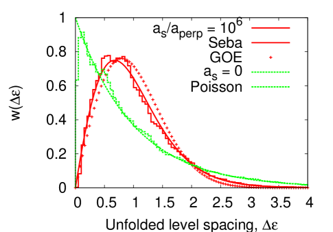
Figure 1: Two bosons in a multimode guide. Nearest-neighbor spacing distribution averaged over $7\times 10^{6}$ eigenstates in the globally unitary regime $a_{s}/a_{\perp}=10^{6}$ and in the regime of no interactions. The Gaussian Orthogonal Ensemble prediction, the Šeba distribution, and the Poisson distribution are shown for comparison. Here and below, $\left(L/a_{\perp}\right)^{2}=2\phi_{gr}\pi^{7}\approx 9774$.

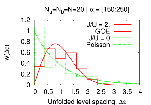
Figure 2: Forty bosons in two wells. Nearest-neighbor spacing distribution averaged over 100 eigenstates in the “maximally chaotic” region $150\leq\alpha\leq 250$. Number of atoms of both type is $N_{a}=N_{b}=N=20$. The $J/U=2$ point corresponds to the empirically broadest fraction of the “chaotic” eigenstates. The case of no hopping is shown as well, along with the Gaussian Orthogonal Ensemble and Poisson predictions. Here and below, the individual coupling constants are $U_{aaR}=0.3041\,U,\,U_{abR}=1.0410\,U,\,U_{bbR}=0.3684\,U,\,U_{aaL}=0.3085\,U,\,U_{abL}=1.4574\,U,\,U_{bbL}=0.4524\,U$.

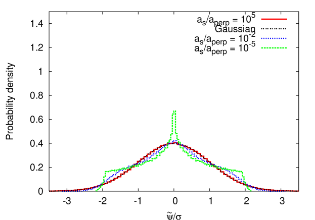
Figure 3: Two bosons in a multimode guide. The probability distribution for value of the eigenstate wavefunction in the region close to the waveguide axis. The eigenstate number $67600$ corresponding to the energy $E_{\alpha}\approx 4.24\times 10^{6}\hbar\omega_{\perp}$ is shown. Since the motion is restricted to the cylindrically symmetric states the reduced wavefunction $\tilde{\psi}(\rho,\,z)\equiv(1/\sqrt{2\pi\rho})\psi(\rho,\,z)$ was used. The Gaussian distribution corresponds to the Berry conjecture. The interaction strengths $a_{s}/a_{\perp}=10^{5}$, $10^{-2}$, and $10^{-5}$ correspond to the unitary, intermediate, and non-interacting regimes respectively. The rest of the parameters is the same as at Fig. 1.

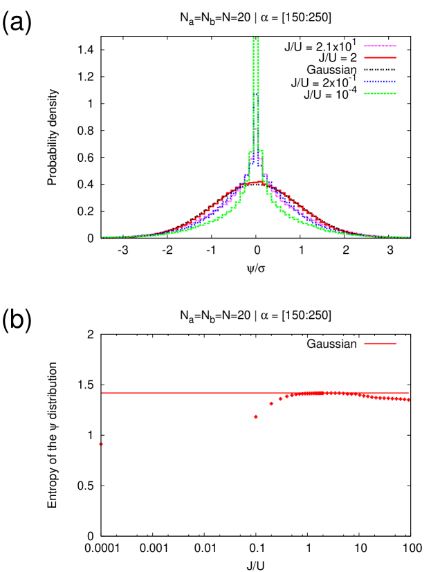
Figure 4: Forty bosons in two wells. (a) The probability distribution for real part of the eigenstate wavefunction on the whole surface of the bi-sphere. The distributions for the individual eigenstates were further averaged over an $150\leq\alpha\leq 250$ window. The distribution is heavily peaked in both integrable limits, $J\ll U$ and $J\gg U$. (b) Entropy of the distribution as a function of the hopping constant. The entropy converges to the Berry conjecture prediction in the region between $J/U\approx 1$ and $J/U\approx 5$. For both (a) and (b) the rest of the parameters is the same as for the Fig. 2.

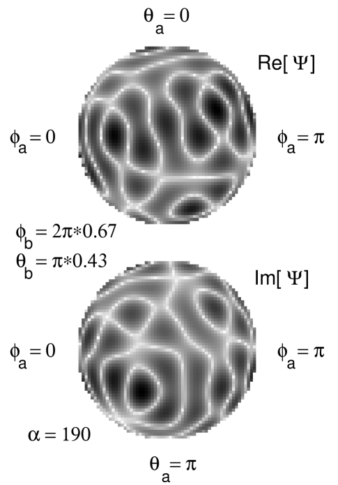
Figure 5: Forty bosons in two wells. The real and imaginary parts of the four-dimensional eigenstate wavefunction living on the surface of a tensor product of two unit spheres. The “maximally chaotic” state $\alpha=190$ is used. The hopping is fixed to $J/U=2$. Even though in both $J\ll U$ and $J\gg U$ limits the eigenstates are strongly polarized, for $J/U=2$ no preferential direction is visible. The rest of the parameters is the same as for the Fig. 2. To enhance contrast, the shading density is made to be proportional to the forth power of the real and imaginary parts respectively.

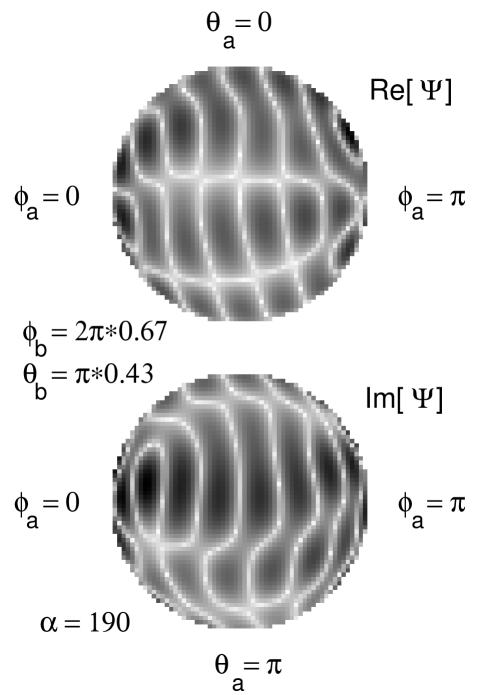
Figure 6: The same as on Fig. 5 but in the regular regime, $J/U=.2$ .

4 Standard quantum-chaotic tests

4.1 Level spacing statistics

The commonly-used measure to access the degree of quantum chaos the shape of level spacing distribution [3]. As usual, the starting point of the procedure is to determine the mean level density to be subsequently removed from the spectral data. The resulting energy spectrum—the so-called unfolded spectrum—does not contain any information specific to the system besides the dimensionless, homogeneous across the spectrum level spacing statistics. This statistics is the principal object of the investigation.

For the case of the waveguide, the mean level density was obtained from the semiclassical approximation to the unperturbed spectrum of the system. Such a simplification was possible due to the fact that for a singular perturbation, the density of states is exactly the same for the interacting and non-interacting systems. For the two-well system, the mean level density was approximated by a fit of the true energy spectrum to a seventh degree polynomial.

The integrable systems exhibit the Poisson statistics of the level spacings, with a peak at zero and an exponential decay at large spacings. One would expect to this type of statistics in a model the energy levels appear under no constraint, besides the given a priori mean level spacing. Indeed, in integrable systems, the energy levels corresponding to different sets of (additional to the energy) integrals of motion can approach each other infinitely closely. It turns out that this property along is sufficient to ensure the Poisson statistics [2, 3].

On the contrary, in a quantum system with no non-trivial integrals of motion, the energy levels tend to repel. This repulsion leads to the appearance of a hole, around zero spacing point, in the level spacing distribution. It is remarkable however that generally, quantum chaotic systems with real Hamiltonians exhibit exactly the same level spacing distribution, namely the one of the Wigner-Dyson type. An ensemble of orthogonal matrices with a Gaussian distribution of the matrix elements (the so-called Gaussian Orthogonal Ensemble (GOE)) serves as a paradigm for this class of Hamiltonians [2, 3].

A multi-dimensional harmonic oscillator constitutes a remarkable exception from the integrable vs. chaotic dichotomy [34]. The unfolded distribution function in this case vanishes at the zero spacing and shows a sharp decay at large spacings. Indeed, we have found that our waveguide system, with a harmonic confinement transversally and a periodic-boundary-conditions box longitudinally, is more sensitive to the effect of a non-integrable perturbation than a seemingly more elegant elongated three-dimensional harmonic oscillator; thus our preference for the former.

The waveguide system shows systematic deviations from the GOE Random Matrix Theory predictions [2]. Note that the unattainability of a complete quantum chaos in singular billiards has been already addressed in the context of the Šeba billiard – flat two-dimensional rectangular billiard with a zero-range scatterer in the middle [1]. Even though the Šeba billiard shows some signatures of the quantum-chaotic behavior, both the level statistics [35, 27, 36] and the momentum distributions in individual eigenstates [37] exhibit substantial deviations from the conventional quantum-chaotic behavior. Our waveguide system belongs to the same class as the Šeba billiard: it is represented by an integrable system perturbed by a separable rank-one perturbation. For both systems, the eigenstates have the “Green’s function” form (5).

The results of the study of the level spacing distribution in the waveguide system are fully consistent with the analogous results for the Šeba billiard [35, 27]. One can show that for $a_{s}\gg a_{\perp}$ (globally unitary regime), the scattering strength reaches the unitary limit for all eigenenergies of the full Hamiltonian. In this regime the distribution quickly converges to the Šeba distribution [35]. This distribution does show a gap at small level spacings but fails to reproduce the Gaussian tail predicted by the GOE. At small $a_{s}$ the level spacing distribution tends to the Poisson one (see Fig. 1). For the energy range $E\gtrsim 100\hbar\omega_{\perp}$ and the aspect ratio $\left(L/a_{\perp}\right)^{2}=2\phi_{gr}\pi^{7}$ the Šeba distribution is approached at $a_{s}\gtrsim 10^{-1}a_{\perp}$.

The level spacing statistics for the two-well system is consistent with the GOE prediction (Fig. 2), even though the statistics is very poor.

4.2 Wavefunction statistics

Another important measure of quantum chaos is the statistics of the wavefunction. Divide the coordinate space of a quantum-chaotic system into regions larger that the de-Broglie wavelength but small enough so that the spatial density does not change substantially across the region. According to the Berry conjecture [4, 5], the coordinate wavefunction should behave, within each region, as a sample from an ensemble of large superpositions of plane waves with random coefficients.

For the waveguide system, we verified that in the globally unitary regime, $a_{s}\gg a_{\perp}$, the statistics of the point-by-point variations of the eigenstate wavefunction in the spatial representation is indeed close to the Gaussian one (Fig. 3), according to Berry’s prediction and a particular observation in the case of the Šeba billiard [1].

The two-well system also behaves according to the Berry conjecture. Fig. 4a presents the distribution of the real part of the wavefunction (14) taken at random points on the bi-sphere and averaged over the eigenstates between $\alpha=150$ and $\alpha=250$. For $J=2$ the distribution is indistinct from the Gaussian. Fig. 4b represents the dependence of the entropy of the distribution on the hopping constant. The entropy converges to the Berry conjecture prediction in the region between $J/U\approx 1$ and $J/U\approx 5$.

Fig. 5 shows the wavefunction of the eigenstate $\alpha=190$ at hopping of $J=2$. This state corresponds to the crossing of all three spectra of the Fig. 9a where the expectation values of the projection of the angular momentum $\hat{\vec{\cal L}}_{a}$ (along with $\hat{\vec{\cal L}}_{b}$) on both $z$ and $x$ axes is small. Accordingly, the nodal structure of the wavefunction appears completely random, with no preferred direction. For comparison, Fig. 6 shows the same state but for weak hopping ($J=.2$) where the motion is expected to be regular.

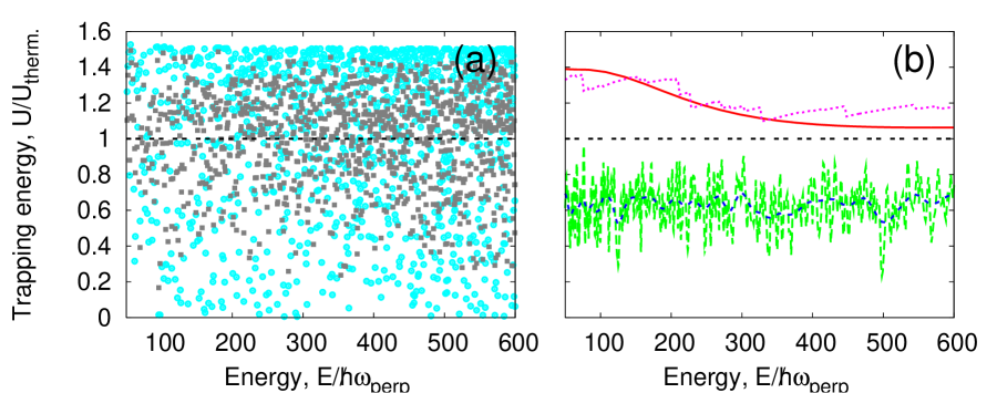
Figure 7: Two bosons in a multimode guide. (a) Quantum expectation value of the trapping energy $U$ for every hundreds eigenstate of the unperturbed Hamiltonian (2) (blue circles) and the full Hamiltonian (1) (grey squares). (b) The time average of the transverse trapping energy $U_{\mbox{\scriptsize relax.}}\equiv\lim_{t_{max}\to\infty}(1/t_{max})\int_{0}^{t_{max}}\!\langle\psi(t)|\hat{U}|\psi(t)\rangle$ after relaxation from an initial state as a function of the energy of the initial state $E$ [see Hamiltonian (1)]. Four families of the initial states are considered. Long-dashed (green) line: state (15) with $n_{0}=0$, $\delta=0.99$, and the energy being controlled via scanning $l_{0}$; short-dashed (blue) line: the same as the previous one, except for $\delta=.1$; dotted (purple) line: the state (15) with $\delta=0.1$ and $l_{0}=0$ and the energy control via $n_{0}$; solid (red) line: state (16) with $\kappa_{2}=2\kappa_{1}$, $\delta=0.99$, $l_{0}=0$ and the energy control via $\kappa_{1}$. All the values of the trapping energy are shown with respect to its microcanonical expectation value $U_{therm.}\approx E/3$. The rest of the parameters is the same as at Fig. 1.

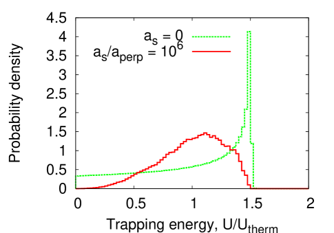
Figure 8: Two bosons in a multimode guide. Probability distribution of the quantum expectation values of the trapping energy $U$ for individual eigenstates of the full Hamiltonian (1) in the globally unitary regime (solid line) and those of the unperturbed Hamiltonian (2) (dashed line). The rest of the parameters is the same as at Fig. 1.

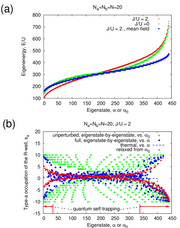
Figure 9: Forty bosons in two wells. (a) Energy spectrum of the Hamiltonian (9) in the absence of hopping ($J/U=0$) and for the hopping $J/U=2$. The spectrum of the mean-field Hamiltonian $\hat{H}_{\mbox{\scriptsize mf}}\equiv\hat{V}+\langle\hat{H}_{0}\rangle$ (see (3), with the hopping as the primary Hamiltonian, is shown as well. The point $\alpha\approx 190$ where all three eigenenergy curves coincide corresponds to the maximal depolarization where the motion is “maximally chaotic”. Here, the density is distributed uniformly over the bi-sphere with no preferred orientation. The labels $\alpha$ and $\alpha_{0}$ correspond to the eigenstates of the full Hamiltonian (9) and the pure-interaction Hamiltonian ($J/U=0$ limit) respectively. (b) Fluctuations of the observable $\hat{s}_{a}\equiv\hat{c}^{\dagger}_{aR}\hat{c}_{aR}-N_{a}/2$. Green crosses correspond to the microcanonical fluctuations in the absence of hopping. Blue crosses correspond to the eigenstate-by-eigenstate fluctuations of the quantum expectation values, suppressed according to the eigenstate thermalization hypothesis. Red crosses give the infinite time average of the quantum expectation for a propagation from an initial state corresponding to one of the eigenstates of the Hamiltonian $\hat{H}_{0}$. The fluctuations of the latter are further suppressed due to an additional averaging of the initial state over the eigenstates. The microcanonical average is shown as the blue dashed line.

5 Eigenstate thermalization phenomenon and the ability to thermalize in a relaxation from an initial state

According to the Eigenstate Thermalization Hypothesis [6, 7, 9, 10], the ability of an isolated quantum system to thermalize follows from suppression of the eigenstate-by-eigenstate fluctuations of the quantum expectation values of relevant observables $\langle\alpha|\hat{A}|\alpha\rangle$ over the eigenstates $|\alpha\rangle$ of the system. Indeed, if one assumes that an observable $\hat{A}$ reaches its thermal value in a time evolution from any initial state with an energy close to a given energy $E$, including the exact eigenstates of the Hamiltonian, then it immediately follows that the matrix elements $\langle\alpha_{1}|\hat{A}|\alpha_{1}\rangle$ and $\langle\alpha_{2}|\hat{A}|\alpha_{2}\rangle$ must be close to each other if the corresponding energies $E_{1}$ and $E_{2}$ are close.

Consider first the system of two particles in a waveguide. As the principal observable of interest, we choose the transverse trapping energy $U$ (see (2)). In our analysis, the potential energy $U$ plays a role of a generic observable in an integrable system: it acts on only one of the degrees of freedom and it has both diagonal and off-diagonal non-zero matrix elements between the eigenstates of the integrable system.

Scattered grey squares at the Fig. 7a show the quantum expectation values of the transverse trapping energy, $\langle\alpha|\hat{U}|\alpha\rangle$, in every hundreds eigenstate (6) of our system (1), relative to its microcanonical expectation value $U_{therm.}\approx E/3$ (in accordance with the energy equipartition between the two harmonic and one free-space degrees of freedom).

Even for the energies much larger than any conceivable energy scale of the system, the variation of $\langle\alpha|\hat{U}|\alpha\rangle$ is only marginally lower than the microcanonical fluctuations in the unperturbed system (2), represented by the blue circles. Figure 8 demonstrates that even though the destruction of the integrals of motion in the interacting system does narrow the distribution of the diagonal matrix elements $\langle\alpha|\hat{U}|\alpha\rangle$ and it does shift the peak towards the microcanonical prediction $U_{therm.}$, the distribution remains relatively broad. We trace this effect to the predicted unattainability of the complete quantum chaos in the singular billiards [35, 36, 38].

Here and below, we assume the globally unitary value of the scattering length, $a_{s}=10^{6}a_{\perp}$.

On the contrary, the behavior of the two-well system is fully consistent with the Eigenstate Thermalization Hypothesis [6, 7, 9, 10] (see Fig. 9b). Here, the observable $\hat{s}_{a}$ (the deviation number of the type-$a$ particles in the right well from $N/2$) is the primary observable of interest. In the window $150\lesssim\alpha\lesssim 250$, all quantum expectation values of $\hat{s}_{a}$ in the eigenstates of the full Hamiltonian (9) are substantially closer to the thermal prediction than their unperturbed counterparts given by the eigenstates $|\alpha_{0}\rangle=|s_{a0},\,s_{b0}\rangle$ of the Hamiltonian (10).

Now we are going to address directly the ability of our system to thermalize from an initial state $|\psi(t\!=\!0)\rangle$. In this case, the infinite time average of the quantum expectation value of an observable $\hat{A}$ will be given by

$$A_{\mbox{\scriptsize relax.}} \equiv \lim_{t_{max}\to\infty}(1/t_{max})\int_{0}^{t_{max}}\!\langle\psi(t)|\hat{A}|\psi(t)\rangle$$

$$= \sum_{\alpha}|\langle\alpha|\psi(t\!=\!0)\rangle|^{2}\langle\alpha|\hat{A}|\alpha\rangle\quad,$$

where $|\alpha\rangle$ are the eigenstates of the system (see [10]).

First, let us attract our attention to the waveguide system.

Consider the following initial state:

$$\langle z|\psi(t\!=\!0)\rangle=C_{\mbox{\scriptsize ax}}\cos{\pi\zeta\over\delta}\theta\left({\delta\over 2}-|\zeta|\right)\cos\left(2\pi l_{0}\zeta\right)|n_{0}\rangle$$ (15)

$$C_{\mbox{\scriptsize ax}}=L^{-1/2}\left[{\delta\over 4}+{1\over 8\pi l_{0}}{\pi^{2}\sin\left(2\pi l_{0}\delta\right)\over\pi^{2}-\left(2\pi l_{0}\delta\right)^{2}}\right]^{-1/2}\,.$$

Longitudinally, the state is represented by the ground state of a length $L\delta$ hard-wall box split initially by an ideal beamsplitter with momenta $\pm 2\pi l_{0}/L$; the box is centered at the maximal interatomic distance. The state is distributed among approximately $\pi/\delta$ axial modes localized about $l=\pm l_{0}$. The initial transverse state is limited to a single mode $n_{0}$. Note that for $n_{0}=0$ and $\delta\approx 1$ the state is conceptually similar to the initial state used in the equilibration experiments [19].

The transverse trapping energy $U$ (see (2)) remains very far from the equilibrium predictions after the relaxation. Fig. 7b shows the equilibrium value of the transverse trapping energy $U$ for three sequences of the initial states of the type (15). For the first two, the energy is controlled via the kinetic energy given by the beamsplitter, while the transverse state is fixed to the ground state. Both show an approximately -40% deviation of the relaxed value of $U$ from the thermal prediction. Note that the initial states of the second sequence have a much greater spread over the longitudinal modes than the first one; consistently, the energy-to-energy variation of the relaxed values of $U$ is less than for the first sequence. In the third sequence, there is no beamsplitting, and the energy is controlled via the initial transverse energy. In this case, the deviation from the thermal prediction ranges between +50% and +5% but never reaches zero.

Another type of the initial state

$$\langle\rho,\,z|\psi(t\!=\!0)\rangle = C_{\mbox{\scriptsize ax}}\cos{\pi\zeta\over\delta}\theta\left({\delta\over 2}-|\zeta|\right)\cos\left(2\pi l_{0}\zeta\right)$$ (16)

$$\times{1\over a{}_{\perp}}\left[{2\kappa_{1}\kappa_{2}\left(\kappa_{1}+\kappa_{2}\right)\over\pi\left(\kappa_{1}-\kappa_{2}\right){}^{2}}\right]^{1/2}\left(e^{-\kappa_{1}\xi}-e^{-\kappa_{2}\xi}\right)$$

allows for an additional spread over the transverse modes. The transverse wavefunction vanishes at the waveguide axis. The mode occupation has a minimum at $n=0$, and the occupation of the ground transverse mode tends to zero when $\kappa_{1}<\kappa_{2}\ll 1$. The results for a sequence similar to the third sequence described above are shown at Fig. 7b as well. In spite of the significant differences in the initial distribution over both the transverse and the longitudinal modes, the deviations from the equilibrium are close to the ones for the third sequence, even though the energy-to-energy variations for the former are less than for the latter.

For our second system, we use the eigenstates of the unperturbed Hamiltonian (10) as the initial states of the relaxation process. The results are shown at Fig. 9b. Here, each red cross shows the infinite time average of the quantum expectation value of the observable $\hat{s}_{a}$ (the deviation of the type-$a$ occupation of the right well from $N_{a}/2$) for a relaxation process originating from the state $|\alpha_{0}\rangle=|s_{a0},\,s_{b0}\rangle$. In the window $150\lesssim\alpha\lesssim 250$ the observable thermalizes fully. Recall, that the eigenstate themalization occurs in the same window.

It is instructive to analyze our results from the point of view of the macroscopic quantum self-trapping, predicted in Refs. [33, 39, 40] and experimentally observed in Ref. [41], for the single-specie two-well bosonic system. From the classical field theory point of view it is a one-dimensional Hamiltonian system similar to a pendulum. Here, the population imbalance between the two wells plays a role of momentum, while the relative phase between the wells plays a role of a coordinate. Similarly to the case of the conventional pendulum, the initial states of sufficiently high momentum preserve the sign of the latter; the time evolution that starts from the states with even higher momentum shows the momentum that almost does not change in time. The states with the opposite sign of the momentum become mutually inaccessible. In terms of the original two-well system, the initial states with the population imbalance higher than a certain critical value preserve the imbalance over time.

The energy landscape for out two-specie two-well system is more complicated. Both the cosine-like dependence of the hopping energy on the relative phases and the hyperbolic shape of the interaction energy surface as a function of the two population imbalances contribute to the potential multi-connectedness of the phase space. At the same time, the initial states used to produce the Fig. 9b are the exact eigenstates of both population imbalances; they leave the relative phases completely uncertain.

We have identified a set of absolutely localized pairs of population imbalances, i.e. the pairs for which no set of imbalances of opposite signature is classically accessible for any pair of initial phases. In particular, the analysis shows that all the unperturbed eigenstates with indices $\alpha_{0}<39$ or $\alpha_{0}>339$ constitute the absolutely localized initial states. This result is consistent with the fully quantum calculation that shows a strong memory of the initial conditions (see Fig. 9b).

6 Summary of results

In this article, we analyze the behavior of two simple atomic systems within two complementary frameworks: quantum chaos and nonequilibrium dynamics. The first system is represented by two short-range-interacting bosonic atoms in a circular, transversely harmonic multimode waveguide. The second is the interacting two-component Bose-Bose mixture in two coupled potential wells. For both systems, we study the level spacing statistics, the statistics of the values of the wavefunction in coordinate representation, degree of the eigenstate thermalization, and the thermalizability in a relaxation from an exited initial state.

For the waveguide system, the wavefunction statistics is fully consistent with the Berry conjecture [4] that predicts a Gaussian distribution for the quantum-chaotic systems. However, the rest of the tests show an incomplete chaotization. We trace this effect to the previously predicted incomplete quantum chaos in the singular billiards [35, 27, 36, 37].

For the double-well system, we identify a quantum-chaotic region of the spectrum that spans, for our set of parameters, about a quarter of the full spectrum. In this part of the spectrum, the system exhibits both strong eigenstate thermalization and the ability to fully thermalize from an initial state.

References

References

- [1] Petr Šeba. Wave chaos in singular quantum billiard. Phys. Rev. Lett., 64(16):1855–1858, 1990.
- [2] O. Bohigas. Random matrix theories and chaotic dynamics. In J. Zinn-Justin M.-J. Gianoni, A. Voros, editor, Chaos and Quantum Physics, Les Houches, session LII. North-Holland, Amsterdam, 1991.
- [3] Thomas Guhr, Axel Müller-Groeling, and Hans A. Weidenmüller. Random-matrix theories in quantum physics: common concepts. Phys. Reps., 299(4-6):189 – 425, 1998.
- [4] M. V. Berry. Regular and irregular semiclassical wavefunctions. J. Phys. A, 10(12):2083–2091, 1977.
- [5] Eric J. Heller. Bound-state eigenfunctions of classically chaotic hamiltonian systems: Scars of periodic orbits. Phys. Rev. Lett., 53(16):1515–1518, 1984.
- [6] A. I. Shnirelman. Ergodic properties of eigenfunctions. Usp. Mat. Nauk, 29(6):181–182, 1974.
- [7] Mario Feingold and Asher Peres. Distribution of matrix elements of chaotic systems. Phys. Rev. A, 34(1):591–595, 1986.
- [8] V. V. Flambaum and F. M. Izrailev. Distribution of occupation numbers in finite fermi systems and role of interaction in chaos and thermalization. Phys. Rev. E, 55(1):R13–R16, 1997.
- [9] J. M. Deutsch. Quantum statistical mechanics in a closed system. Phys. Rev. A, 43(4):2046–2049, 1991.
- [10] Mark Srednicki. Chaos and quantum thermalization. Phys. Rev. E, 50(2):888–901, 1994.
- [11] G. P. Berman, F. Borgonovi, F. M. Izrailev, and A. Smerzi. Irregular dynamics in a one-dimensional bose system. Phys. Rev. Lett., 92(3):030404, 2004.
- [12] Pasquale Calabrese and John Cardy. Quantum quenches in extended systems. J. Stat. Mech., page P06008, 2007.
- [13] V. V. Flambaum and F. M. Izrailev. Entropy production and wave packet dynamics in the fock space of closed chaotic many-body systems. Phys. Rev. E, 64(3):036220, 2001.
- [14] Corinna Kollath, Andreas M. Läuchli, and Ehud Altman. Quench dynamics and nonequilibrium phase diagram of the bose-hubbard model. Phys. Rev. Lett., 98(18):180601, 2007.
- [15] S. R. Manmana, S. Wessel, R. M. Noack, and A. Muramatsu. Strongly correlated fermions after a quantum quench. Phys. Rev. Lett., 98(21):210405, 2007.
- [16] Marcos Rigol, Vanja Dunjko, and Maxim Olshanii. Thermalization and its mechanism for generic isolated quantum systems. Nature, 452(7189):854–858, 2008.
- [17] K. Sengupta, Stephen Powell, and Subir Sachdev. Quench dynamics across quantum critical points. Phys. Rev. A, 69(5):053616, 2004.
- [18] Anatoli Polkovnikov and Vladimir Gritsev. Breakdown of the adiabatic limit in low-dimensional gapless systems. Nature Physics, 4(6):477–481, 2008.
- [19] Toshiya Kinoshita, Trevor Wenger, and David S. Weiss. A quantum Newton’s cradle. Nature, 440(7086):900–903, 2006.
- [20] S. Hofferberth, I. Lesanovsky, B. Fischer, T. Schumm, and J. Schmiedmayer. Non-equilibrium coherence dynamics in one-dimensional bose gases. Nature, 449(7160):324–327, 2007.
- [21] S. Hofferberth, I. Lesanovsky, T. Schumm, A. Imambekov, V. Gritsev, E. Demler, and J. Schmiedmayer. Probing quantum and thermal noise in an interacting many-body system. Nature Physics, 4(6):489–495, 2008.
- [22] Lea F. Santos and Marcos Rigol. Onset of quantum chaos in one-dimensional bosonic and fermionic systems and its relation to thermalization. arXiv:0910.2985, 2009.
- [23] Vladimir A. Yurovsky and Maxim Olshanii. Restricted thermalization for two interacting atoms in a multi-mode harmonic waveguide. arXiv:1001.0225, 2010.
- [24] S. Albeverio and P. Kurasov. Singular perturbations of differential operators : solvable Schröinger type operators. Number 271 in London Mathematical Society lecture note series. University Press, Cambridge, 2000.
- [25] M. Olshanii. Atomic scattering in the presence of an external confinement and a gas of impenetrable bosons. Phys. Rev. Lett., 81(5):938–941, 1998.
- [26] M. G. Moore, T. Bergeman, and M. Olshanii. Scattering in tight atom waveguides. J. Phys. IV (France), 116:69–86, 2004.
- [27] S Albeverio and P Šeba. Wave chaos in quantum-systems with point interaction. J. Stat. Phys., 64(1-2):369–383, 1991.
- [28] T Busch, BG Englert, K Rzazewski, and M Wilkens. Two cold atoms in a harmonic trap. Foundations of Physics, 28(4):549, 1998.
- [29] Vladimir A. Yurovsky, Maxim Olshanii, and David S. Weiss. Collisions, correlations, and integrability in atom waveguides. In Adv. At. Mol. Opt. Phys., volume 55, pages 61–138. Elsvier Academic Press, New York, 2008.
- [30] Z. Idziaszek and T. Calarco. Two atoms in an anisotropic harmonic trap. Phys. Rev. A, 71(5):050701(R), 2005.
- [31] E. L. Bolda, E. Tiesinga, and P. S. Julienne. Pseudopotential model of ultracold atomic collisions in quasi-one- and two-dimensional traps. Phys. Rev. A, 68(3):032702, 2003.
- [32] K. Kanjilal, John L. Bohn, and D. Blume. Pseudopotential treatment of two aligned dipoles under external harmonic confinement. Phys. Rev. A, 75(5):052705, 2007.
- [33] G. J. Milburn, J. Corney, E. M. Wright, and D. F. Walls. Quantum dynamics of an atomic bose-einstein condensate in a double-well potential. Phys. Rev. A, 55:4318, 1997.
- [34] C. B. Whan. Hierarchical level-clustering in two-dimensional harmonic oscillators. Phys. Rev. E, 55(4):R3813–R3816, 1997.
- [35] P. Šeba and K. Życzkowski. Wave chaos in quantized classically nonchaotic systems. Phys. Rev. A, 44(6):3457–3465, 1991.
- [36] E. Bogomolny, Ulrich Gerland, and C. Schmit. Singular statistics. Phys. Rev. E, 63:036206, 2001.
- [37] G. Berkolaiko, J. P. Keating, and B. Winn. Intermediate wave function statistics. Phys. Rev. Lett., 91(13):134103, 2003.
- [38] E. Bogomolny, O. Giraud, and C. Schmit. Nearest-neighbor distribution for singular billiards. Phys. Rev. E, 65(5):056214, 2002.
- [39] A. Smerzi, S. Fantoni, S. Giovanazzi, and S. R. Shenoy. Quantum coherent atomic tunneling between two trapped bose-einstein condensates. Phys. Rev. Lett., 79(25):4950–4953, 1997.
- [40] S. Raghavan, A. Smerzi, S. Fantoni, and S. R. Shenoy. Coherent oscillations between two weakly coupled bose-einstein condensates: Josephson effects, oscillations, and macroscopic quantum self-trapping. Phys. Rev. A, 59(1):620–633, 1999.
- [41] Michael Albiez, Rudolf Gati, Jonas Fölling, Stefan Hunsmann, Matteo Cristiani, and Markus K. Oberthaler. Direct observation of tunneling and nonlinear self-trapping in a single bosonic josephson junction. Phys. Rev. Lett., 95(1):010402, 2005.