The triaxial ellipsoid dimensions, rotational pole, and bulk density of ESA Rosetta target asteroid (21) Lutetia

Abstract

Context. Asteroid (21) Lutetia is the target of the ESA Rosetta mission flyby in 2010 July.

Aims. We seek the best size estimates of the asteroid, the direction of its spin axis, and its bulk density, assuming its shape is well described by a smooth featureless triaxial ellipsoid, and to evaluate the deviations from this assumption.

Methods. We derive these quantities from the outlines of the asteroid in 307 images of its resolved apparent disk obtained with adaptive optics (AO) at Keck II and VLT, and combine these with recent mass determinations to estimate a bulk density.

Results. Our best triaxial ellipsoid diameters for Lutetia, based on our AO images alone, are $a\times b\times c=132\times 101\times 93$ km, with uncertainties of $4\times 3\times 13$ km including estimated systematics, with a rotational pole within 5^∘ of ECJ2000 [$\lambda\ \beta$] = [$45^{\circ}-7^{\circ}$], or EQJ2000 [RA DEC] = [$44^{\circ}\ +9^{\circ}$]. The AO model fit itself has internal precisions of $1\times 1\times 8$ km, but it is evident, both from this model derived from limited viewing aspects and the radius vector model given in a companion paper, that Lutetia has significant departures from an idealized ellipsoid. In particular, the long axis may be overestimated from the AO images alone by about 10 km. Therefore, we combine the best aspects of the radius vector and ellipsoid model into a hybrid ellipsoid model, as our final result, of $124\pm 5\times 101\pm 4\times 93\pm 13$ km that can be used to estimate volumes, sizes, and projected areas. The adopted pole position is within 5^∘ of [$\lambda\ \beta$] = [$52^{\circ}-6^{\circ}$] or [RA DEC] = [$52^{\circ}\ +12^{\circ}$].

Conclusions. Using two separately determined masses and the volume of our hybrid model, we estimate a density of $3.5\pm 1.1$ or $4.3\pm 0.8$ g cm^-3. From the density evidence alone, we argue that this favors an enstatite-chondrite composition, although other compositions are formally allowed at the extremes (low-porosity CV/CO carbonaceous chondrite or high-porosity metallic). We discuss this in the context of other evidence.

1 Introduction

The second target of the ESA Rosetta mission, asteroid (21) Lutetia, had a favorable opposition in 2008-09, reaching a minimum solar phase angle of $\omega=0.45\degr$ on 2008 November 30, and a minimum distance from the Earth of 1.43 AU a week earlier. Based on previously determined sizes of Lutetia, with diameters ranging from 96 km from IRAS [Tedesco et al. 2002, 2004] to 116 km from radar Magri et al. [1999, 2007], Lutetia should have presented an apparent diameter of 0.10″, slightly more than twice the diffraction limit of the Keck Observatory 10 m telescope at infrared wavelengths (1-2 $\mu$m). Continuing our campaign [Conrad et al. 2007; Drummond et al. 2009; Carry et al. 2010a] to study asteroids resolved with the world’s large telescopes equipped with adaptive optics (AO), we have acquired more than 300 images of Lutetia, most from the 2008-09 season. An exceptionally good set of 81 images was obtained on 2008 December 2 with the Keck II telescope, which, despite the high sub-Earth latitude, yields a full triaxial ellipsoid solution from the changing apparent ellipses projected on the plane of the sky by the asteroid. Analyzing all available images (2000, 2007, and 2008-09 seasons) yields a result consistent with the December 2 set.

2 Observations

Table 1 gives the observing circumstances for all seven observation dates, where, in addition to the date, Right Ascension, Declination, and Ecliptic longitudes and latitudes of Lutetia, we give its Earth and Sun distance, the solar phase angle ($\omega$), the position angle of the Sun measured east from north while looking at the asteroid (NTS), the filter and the number of images ($m$) used to form mean measurements at $n$ epochs, the scale in km/pix at the distance of the asteroid on the date, and the instrument and telescope configurations used for the observations as listed in Table 2. Multiplying the first scale in Table 1 by the scale in Table 2 will give a km/$\arcsec$ scale at the distance of the asteroid, and multiplying this by the appropriate resolution element ($\Theta$) from Table 2, which is the diffraction limit $\Theta=\lambda/D$, where $\lambda$ is the wavelength and $D$ is the telescope diameter, gives the last column of Table 1, the km per resolution element scale.

The best data set, obtained at K^′ on December 2, comprises images at 9 epochs, 9 images per epoch, where each image is a 0.4 second exposure. Figure 1 shows a single image from each of the 9 epochs, and clearly reveals the asteroid rotating over a quarter of its 8.2 h period.

Figure 2 illustrates the range of solar phase angles for our observations, showing that on more than half of the dates the phase angle was greater than $17\degr$, which, for irregular bodies, can lead to violations of the assumptions we adopt in Section 3. In this particular case, however, we have found the data are still quite useful and contribute substantially to our final results.

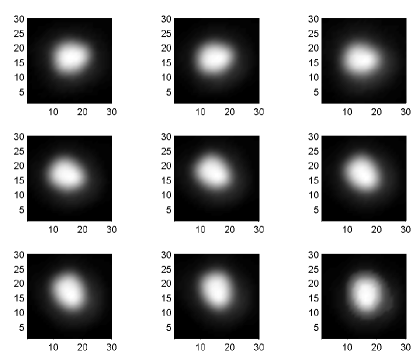
Figure 1: Sample AO images of Lutetia at nine epochs on 2008 December 2. The scale is in pixels, where 1 pixel corresponds to 0.01″. North is up and east is to the left. Images are displayed on a linear scale, after bi-linear interpolation. From left to right, top to bottom, the images were obtained between 6:52 and 9:01 UT after subtracting for light-time travel. They correspond to the 9 points in Fig  3.

Table 1: Observation Log for (21) Lutetia

Date	EQJ2000	ECJ2000	V	Earth	Sun	$\omega$	NTS	Filter	Scale1	Config	Scale2
(UT)	(RA° Dec°)	(Lon° Lat°)		(AU)	(AU)	(°)	(°)	(m/n)	(km/pix)	Table 2	(km/rex)
Aug 15, 2000	12.3 $-\phantom{0}0.3$	11.2 $-5.1$	10.5	1.239	2.057	21.6	71.6	K′(19/1)	15.10	A	39.8
Jun 26, 2007	246.0 $-20.7$	247.8 $+0.9$	10.1	1.295	2.305	3.3	286.4	Ks(35/7)	12.47	B	51.7
Oct 22, 2008	75.1 $+20.9$	76.2 $-1.8$	11.2	1.555	2.352	17.9	85.9	J  (15/2)	11.21	C	29.3
Oct 22, 2008	75.1 $+20.9$	76.2 $-1.8$	11.2	1.555	2.352	17.9	85.9	H  (15/2)	11.21	C	38.3
Oct 22, 2008	75.1 $+20.9$	76.2 $-1.8$	11.2	1.555	2.352	17.9	85.9	K′(33/3)	11.21	C	49.6
Nov 21, 2008	69.4 $+20.8$	70.9 $-1.3$	10.5	1.430	2.406	4.7	88.5	K′(  4/1)	10.31	C	45.6
Dec 22, 2008	66.4 $+20.6$	68.1 $-1.1$	10.2	1.441	2.426	1.1	236.7	K′(81/9)	10.39	C	46.0
Jan 23, 2009	59.6 $+20.6$	61.9 $+0.1$	11.8	1.895	2.518	20.1	258.5	K′(30/2)	13.66	C	60.5
Feb 22, 2009	60.6 $+20.9$	62.8 $+0.2$	12.0	2.033	2.534	21.5	258.9	H  (30/2)	14.66	C	81.1
Feb 22, 2009	60.6 $+20.9$	62.8 $+0.2$	12.0	2.033	2.534	21.5	258.9	K′(45/3)	14.66	C	64.9

Table 2: Configuration for Table 1

Configuration	Instrument	Telescope	Aperture	Scale	Filter	Wavelength	Resolution
			(m)	(pix/″)		($\mu$m)	(″)
A	NIRSPEC	Keck II	10	59.52	K′	2.12	0.044
B	NACO	ESO VLT UT4	8.2	75.36	Ks	2.18	0.055
C	NIRC2	Keck II	10	100.6	J	1.25	0.026
					H	1.63	0.034
					K′	2.12	0.044

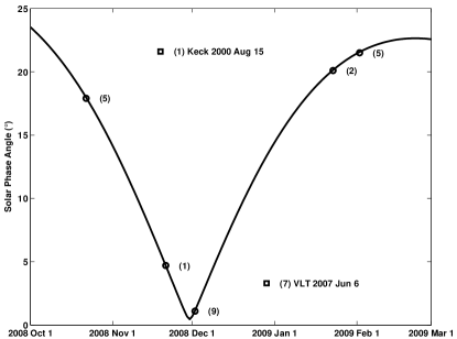
Figure 2: Range of solar phase angles ($\omega$) for (21) Lutetia observations. All (circles) but two dates (squares) are from the 2008-09 opposition. We list the date and observatory for observations obtained outside the 2008-09 campaign. The number of epochs for each date are listed in parentheses.

3 Analysis

Assuming that an asteroid can be modeled as a uniformly illuminated triaxial ellipsoid rotating about its short axis, it is possible to estimate its diameters ($a\geq b\geq c$) and find the direction of its spin axis from the observation of a series of ellipses projected as it rotates. We can thus treat any asteroid in the same manner as we treat asteroids that are well described by the triaxial assumption, e.g., those that we have defined as Standard Triaxial Ellipsoid Asteroids, or STEAs [Drummond et al. 1985, 1998, 2009; Conrad et al. 2007; Drummond & Christou 2008]. The key to turning the projected ellipses into a triaxial ellipsoid is determining the ellipse parameters from AO images. We use the method of Parametric Blind Deconvolution [PBD, Drummond et al. 1998; Drummond 2000] to find the long ($\alpha$) and short ($\beta$) projected (plane of sky) ellipse axes dimensions and the orientation or position angle (PA) of the long axis. PBD allows us to find not only the asteroid ellipse parameters but parameters for the Point Spread Function (PSF) as well. Having shown that a good model for the AO PSF is a Lorentzian [Drummond et al. 1998; Drummond 2000] we simply treat a disk-resolved image of an asteroid as the convolution of a flat-topped ellipse and a Lorentzian, making a simultaneous fit for each in the Fourier plane where the convolution becomes a simple product.
All 307 images were fit for the projected asteroid ellipse parameters and individual Lorentzian PSFs. The mean and standard deviations of the parameters were formed around epochs consisting of a series of 3 to 15 images obtained in one sitting at the telescope. We then solve the triaxial ellipsoid from a least square inversion of the ellipse parameters [Drummond et al. 1985; Drummond 2000].

The projected ellipse parameters can also be extracted from images deconvolved with an alternate algorithm such as Mistral [Conan et al. 2000; Mugnier et al. 2004]. Such contours provide a direct measurement of details of the projected shape of the asteroid, allowing the construction of the radius vector model that we present in Carry et al. [2010b], providing a more refined description of the shape of Lutetia. However, only the PBD parameters were used in deriving ellipsoid solutions here.
While observations from one night can produce triaxial ellipsoid results [Conrad et al. 2007; Drummond & Christou 2008; Drummond et al. 2009] it is possible to combine observations from different nights over multiple oppositions to make a global fit if a sidereal period is known with enough accuracy (Drummond et al. in preparation). This can resolve the natural two-fold ambiguity in the location of a rotational pole from a single night of data (see Section 4.2), and in some cases reduce the uncertainty in the triaxial ellipsoid dimensions if the asteroid is observed over a span of sub-Earth latitudes. For instance, when observations are restricted to high sub-Earth latitudes, even a few images at an equatorial aspect will supply a much better view of the $c$ axis than a long series at near polar aspects. In other words, different viewing geometries generally lead to a better solution.
Unfortunately, during the last two oppositions, in 2007 and 2008-09, Lutetia’s positions were $\sim 180\degr$ apart on the celestial sphere. In fact, the position of Lutetia for the Very Large Telescope (VLT) observations on 2007 Jun 6 was exactly $180\degr$ from its position on 2008 December 2 (see Table 1), which meant that regardless of the location of the rotational pole, the two sets of observations were obtained at the same sub-Earth latitude, but of opposite signs. Thus, with the now-known pole, our observations of Lutetia over the 2008-09 opposition were at the same (but southerly) deep sub-Earth latitudes as the VLT observations in the previous (but northerly) deep sub-Earth latitude opposition in 2007, affording the same view of the strongly fore-shortened $c$ axes, but from the opposite hemisphere. The single set of images in 2000 was also obtained at deep southerly latitudes. Thus, we have no equatorial view of Lutetia and, therefore, its shortest ($c$) dimension remains less well determined than the other two.

4 Results

4.1 Ellipsoid Fits

We made two separate fits to our data, one using only our best data set from December 2, and the other combining all of our data taken over the 8.5 year span using a sidereal period of 8.168 27 h from Carry et al. [2010b] to link them together. The results of these two fits give highly consistent values for the equatorial dimensions, but not for $c$. When fitting all of the data, a higher $c$ value is preferred, but we restrict $c$ to the usual physical constraint of $b\geq c$. Because the entire data set, taken as an ensemble, has higher noise, we consider the $b=c$ as a limiting case (a biaxial ellipsoid), and adopt the value of c derived from the Dec 2 data alone as our preferred value. Both solutions are listed in Table 3, where $\theta$ is the sub-Earth latitude, $PA_{Node}$ is the position angle of the line of nodes measured east from north, and $\psi_{0}$ is rotational phase zero, the time of maximum projected area when the $a$ axis lies unprojected in the plane of the sky. The uncertainties shown in Table 3 are the internal precisions of the model fit, and do not include systematics. We have assigned overall uncertainties to our ellipsoid model, including systematics, of $4\times 3\times 13$ km in the dimensions, and 5$\degr$ in the pole position.

Table 3: (21) Lutetia Ellipsoid Fit Solutions

	Triaxial (Dec 2008)	Biaxial (All)
a (km)	132$\pm$1	132$\pm 1$
b (km)	101$\pm$1	101$\pm 1$
c (km)	93 $\pm$8	c=b
$\theta$ (°)	$-66\pm$3	$-59\pm 3$
$PA_{Node}(\degr)$	155$\pm 3$	178$\pm 6$
$\psi_{0}$ (Max) (UT)	5.66$\pm 0.07$	5.10$\pm 0.12$
Pole
[RA°; Dec°]	[44;+9]	[34; +16]
$\sigma$ radius (°)	2.5	3.1
[$\lambda\degr;\beta\degr$]	[45;-7]	[37; +3]

Table 4: RMS of Projected Ellipses from Models

	$\alpha$	$\beta$	PA	Fig
	(km)	(km)	(°)
Triaxial (2008 Dec only)	0.4	0.9	1.1	3
Triaxial (All)	4.1	4.7	6.9	4
Biaxial (All)	3.4	4.4	6.6	5

Figure 3 shows the triaxial ellipsoid fit to the December data. Figure 4 shows the residuals from the prediction using the December triaxial ellipsoid model for all of the data, and Figure 5 shows the overall residuals to the biaxial fit. The difference between Figs 4 and 5 is subtle, showing that Lutetia is close to a prolate ellipsoid. Trends in some of the residuals, such as the curling set of position angles at the right of the top plot in Fig 4, and at the left of the similar plot in Fig 5, indicate departures from our assumptions of a smooth featureless ellipsoid rotating about its short axis, and motivate the more detailed shape model that we present in Carry et al. [2010b]. The rms weighted (by the observational uncertainty of each measurement) residuals for $\alpha$ and $\beta$, the projected ellipse major and minor axes lengths, and the weighted residuals for the position angle (PA) of the long axis, are given in Table 4, and are to be associated with Figs 3-5. These can be interpreted as uncertainties (but without possible systematics) for any predicted future projected ellipse parameters.

The axial ratios derived from our model are $a/b=1.32$ and $b/c=1.09$. From a compilation of axial ratios and rotational poles, mostly from lightcurves, the average axial ratios are $a/b=1.27\pm 0.06$ and $b/c=1.45\pm 0.55$, both within one sigma of our directly determined values. More recent work suggests a $b/c$ ratio of less than 1.1 [Belskaya et al. 2010], also consistent with our value. Our fit of the radius vector model derived from lightcurves by Torppa et al. [2003, see section 5 below] yields an $a/b$ ratio of $1.17$ and $b/c=1.18$, and the latest radius vector model derived by Carry et al. [2010b] from a combination of present AO images and lightcurves has ratios of 1.23 and 1.26. Our hybrid model, given as the final result of our paper here (see next section), has $a/b=1.23$ and $b/c=1.09$.

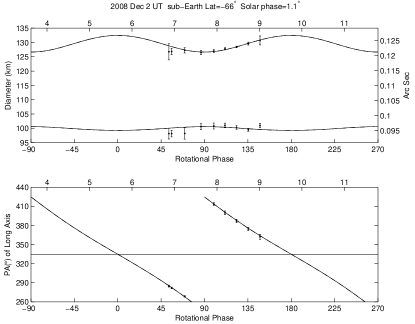
Figure 3: Triaxial ellipsoid fit to measured ellipse parameters of (21) Lutetia on 2008 Dec 2. In the upper subplot, each image’s long ($\alpha$) and short ($\beta$) axis dimensions are plotted as dots with $1\,\sigma$ uncertainties. The lines are the prediction for the projected ellipses from the triaxial ellipsoid parameters in Table 3, derived from the fit to the data. Because the solar phase angle ($\omega$) is only 1.1° (Fig. 2 and Table 1), the ellipse parameters for the terminator ellipse is coincident with the projected ellipse lines. The lower subplot shows the same for the position angle of the long axis, where the horizontal line is the line of nodes, the intersection of the asteroid’s equator and the plane of the sky. This figure is corrected for light time travel, i.e., the plot is in the body-centered time frame.

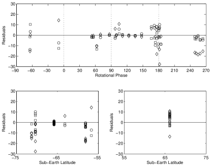
Figure 4: Residuals between the triaxial ellipsoid model (obtained from December 2008 observations only) and all observations as function of the rotation phase and latitude. The major and minor axes residuals are shown as squares and circles, respectively, both in km, and the position angle residuals, in degrees, are shown as diamonds. From Table 4, the rms of the weighted residuals are 4.1 and 4.7 km for the major and minor axes, respectively, and 6.9^∘ for the position angle. The data in the northern hemisphere is from the VLT in 2007.

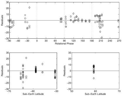
Figure 5: Same as previous figure, except that the residuals are between the biaxial ellipsoid model and the data. From Table 4, the rms of the weighted residuals are 3.4 and 4.4 km for the major and minor axes, respectively, and 6.6^∘ for the position angle.

4.2 Rotational Pole

There is a natural two-fold ambiguity in the location of the rotational pole with our method that is symmetric with respect to the position of the asteroid if observed on one night. Thus, there are two possible poles for the December triaxial ellipsoid solution. However, if the asteroid can be observed at significantly different positions, then the rotational pole can be disambiguated. The single 2000 observation helps break the ambiguity since the residuals are some 18% higher for the rejected pole than for the accepted region when considering all of the data. Otherwise, the 2008-09 observations and the 2007 data from the same positions, would not have provided enough diversity to break the ambiguity.

The poles from various lightcurve techniques can have two- or four-fold ambiguities [see Magnusson et al. 1989, for a good summary], which can be broken when paired with our results. Figure 6 shows the positions of about half of the poles (see footnote 1) found from lightcurve methods (the other half lie on the opposite hemisphere), as well as ours. We assert that the correct region for the pole location is where our poles near $RA=45\degr$ coincide with the span of lightcurve poles in this hemisphere. Furthermore, the lightcurve inversion (LCI; see section 5) pole of Torppa et al. [2003] lies at coordinates RA$=52^{\circ}$ and Dec$=+13^{\circ}$, less than $9^{\circ}$ from our triaxial ellipsoid pole in Table 3.

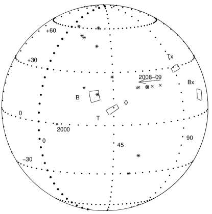
Figure 6: Pole locations for Lutetia on the celestial globe. The positions of Lutetia on the sky for the seven nights of our observations are indicated by $\times$’s. The opposite of the 2007 position is the circle on top of the $\times$ for December 2008. The poles found from lightcurve work are marked with asterisks, with the LCI pole [Torppa et al. 2003] shown as a diamond (our final pole, the KOALA pole [Carry et al. 2010b], is less than a degree from the LCI pole). The four wedge shaped areas are the uncertainty regions around our poles, with T and B indicating our two each possible triaxial and biaxial ellipsoid solution poles. Our rejected poles are marked as Bx and Tx at the far right, while the lightcurve rejected pole region is on the other side of the globe.

5 Comparison with Lightcurve Inversion Model

Figure 7 shows our PBD images of Lutetia from 2008 December 2. Each image is the mean of 9 shifted and added images at each epoch, and then linearly deconvolved of the Lorentzian PSF found in its fit. Notice the tapered end.

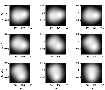
Figure 7: Same as Fig 1, except PBD (deconvolved) images of (21) Lutetia from 2008 December 2.

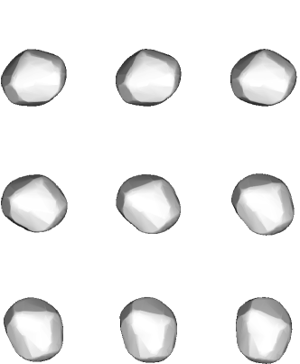
Figure 8: Convex shape model of (21) Lutetia from Torppa et al. [2003], plotted at same times as Fig 7.

For comparison, the lightcurve inversion model (see footnote 2) based on the work of Torppa et al. [2003] is shown in Fig 8 for the same times. The model appears to match the overall shape and orientation in the images, verifying the pole and sidereal period, but it does appear fatter and less tapered than the images of the asteroid. In a following article we combine our AO images with lightcurve data using a method known as KOALA (Knitted Occultation, Adaptive-optics, and Lightcurve Analysis [Carry et al. 2010b]) to produce an improvement over the previous LCI model. Not only does it yield better matches to the AO images, but it provides an absolute kilometer scale, and it can reproduce Lutetia’s lightcurve history.

Although a triaxial ellipsoid fit of the new KOALA model yields diameters of $124\times 101\times 80$, the model is very non-ellipsoid in appearance, and while the $b$ diameter is in agreement between the AO-only and the KOALA model, both the KOALA $a$ and $c$ dimensions are $\sim 10$ km smaller than from our triaxial ellipsoid results here. The AO-only triaxial ellipsoid solution comes from only a quarter of a rotation, when the minimum area is projected (over what would be a lightcurve minimum). During the time of the 2008 Dec 2 AO observations, the $b$ axis was seen unprojected in the plane of the sky, but both the $a$ and $c$ axes were not. It is the extrapolation, as it were, in rotation to the maximum projected area, when the $a$ axis could be seen unprojected, that leads to an $a$ dimension larger than found from KOALA. The KOALA technique, by combining lightcurves that cover all rotational phases and sub-Earth latitudes with the AO images (at restricted rotational phases and latitudes), finds that there is a large depression on the side of Lutetia away from the 2008 Dec 2 observations that was not completely sampled by our imaging, resulting in the smaller KOALA model $a$ axis dimension. This depression of $\sim 10$ km explains the difference between the two $a$ dimensions.

On the other hand, since KOALA only uses amplitudes from lightcurves, and since amplitudes are a strong function of $a/b$ but a weak function of $b/c$, the KOALA model $c$ dimension is only weakly determined when the AO images at high sub-Earth latitudes only reveal a strongly foreshortened $c$ axis. (See [Carry et al. 2010b] for a discussion on the limits of the KOALA inversion in the particular case of Lutetia.) Therefore, Lutetia’s $c$ dimension is best determined from the 2008 December 2 AO data set.

To make the best possible model for use in evaluating sizes, cross-sectional areas, volumes, and densities, we combine what we consider the best aspects of both models into a hybrid triaxial ellipsoid/KOALA model that has dimensions of $124\times 101\times 93$ km, taking the $a$ diameter from KOALA and the $c$ diameter from the AO triaxial ellipsoid fit. The original KOALA model radius vector $Z$ components are merely expanded by 93/80. We estimate the uncertainties on these dimensions, including possible systematics, to be $5\times 4\times 13$ km. Our best final average diameter is, then, $(abc)^{1/3}=105\pm 5$ km. The rotational pole for these hybrids should be the KOALA pole at [RA Dec]=[$52^{\circ}\ +12^{\circ}$], since it is primarily based on lightcurves obtained over 47 years as opposed to the triaxial ellipsoid pole in Table 3 from nine epochs on 2008 December 2, although they are less than 8^∘ apart. The uncertainty for this pole is about $5^{\circ}$ in each coordinate.

6 Taxonomy and Density

Lutetia was well observed in the 1970s, yielding visible and near-infrared reflectance spectra [McCord & Chapman 1975], radiometric albedos and diameter estimates [Morrison 1977], and polarimetric albedos and diameter estimates [Zellner & Gradie 1976], which have been confirmed by similar observations reported during the last decade [see review by Belskaya et al. 2010]. Based on these data, Chapman et al. [1975] placed only three asteroids, (16) Psyche, (21) Lutetia, and (22) Kalliope, into a distinct taxonomic group to which Zellner & Gradie [1976] assigned the letter “M”. The M type was defined in terms of spectral and albedo properties by Bowell et al. [1978], who assigned a diameter of 112 km to Lutetia (estimates by Morrison [1977] and Zellner & Gradie [1976] had been diameters of 108–109 and 110 km, respectively).
It was later found by radar that some, but not all, M-types were metallic. Rivkin et al. [1995] recognized that there were two sub-types of M-type asteroids. The standard M types showed high radar reflectivity and relatively neutral colors, both apparently due to metal. The other type (also showing similar colors, but now thought to be due to metal flakes embedded in a colorless stony matrix) had a 3 micron band, ascribed to hydrated minerals and which was deemed to be unlikely on a chiefly metallic body. Rivkin et al. [1995] called this new “wet” subclass M(W) and assigned Lutetia to this subclass [Rivkin et al. 2000]. Chapman & Salisbury [1973] first suggested that what we now term an M-type spectrum might be associated with enstatite chondrites (ECs) and Rivkin et al. [2000] suggested a hydrated EC as a plausible composition for Lutetia. Recently, Vernazza et al. [2009] and (partly) Nedelcu et al. [2007] showed that ECs are a good match for the visible/near-infrared spectra of Lutetia.
The measured visual albedo for Lutetia has typically ranged over 15–22%, much higher than for the more common (CI/CM) carbonaceous chondrites (CC) and overlapping the lower range for S-types (in recent literature, the early dedicated observations of Lutetia have been supplanted by reference to five rather inconsistent IRAS scans, which imply a still higher albedo and smaller effective diameter for Lutetia, well under 100 km, to which we assign less significance, especially because they are inconsistent with the mean size derived here). The radiometry by Mueller et al. [2006], reduced using two different thermal models, also yields albedos too high for most CC meteorites. A recent determination of visual albedo, using Hubble Space Telescope observations [Weaver et al. 2009] and the size/shape/pole results from the present paper and Carry et al. [2010b], indicate a value near 16%. This value, consistent with EC albedos (as well as metallic), is generally higher than most CCs, although some types of CCs, namely CO/CVs, have higher albedos, typically about 10%, with some COs getting as high as 15–17% [Clark et al. 2009].
Radar observations of Lutetia (Magri et al. [1999, 2007], confirmed by Shepard et al. [2008]) showed that Lutetia has a moderate radar albedo (0.19–0.24), comfortably in the mid-range of ECs, but considerably lower than metallic M-types and higher than most CCs. The uncertainty range in these values overlaps with some CO/CV carbonaceous chondrites compositions at the low extreme and with some metallic compositions at the high end. Hence, CO/CV carbonaceous chondrites cannot be ruled out based on albedo considerations alone.
Indeed, numerous researchers in the last few years (Lazzarin et al. [2004, 2009, 2010]; Barucci et al. [2005]; Birlan et al. [2006]; Barucci et al. [2008]; Perna et al. [2010], see summary by Belskaya et al. [2010]) have argued that Lutetia shows certain spectral characteristics (e.g., in the thermal IR) that resemble CO and CV types and do not resemble a metallic meteorite. However, in these studies, the comparisons with EC meteorites was less thorough, partly because mid-infrared comparison data are not extensive. From rotationally resolved visible/near-infrared spectra of Lutetia, Nedelcu et al. [2007] claimed a better match with CC in one hemisphere and with EC in the other, although this has yet to be confirmed. If Lutetia were highly heterogenous, that might explain some of the conflicting measurements.
Vernazza et al. [2010], however, have shown that mid-infrared emission of asteroids of similar composition can be very different due to differences in surface particle size. Mineralogical interpretations from this wavelength range are thus subject to caution and must be supported by VNIR reflectance spectra. Also, although some CO meteorites show albedos approaching that of Lutetia, the lack of a 1 micron olivine band in Lutetia’s reflectance spectrum [see Fig. 3 of Barucci et al. 2005] argues against CO composition since most, but not all, COs have a 1 micron band. Since the strength of this band generally shows a positive correlation with albedo, Lutetia’s high albedo suggests that a strong 1 micron band should be present if its composition were CO. The lack of a drop-off in Lutetia’s spectral reflectance below 0.55 micron and its high albedo make it inconsistent with CV meteorites [see Gaffey 1976, for instance]. Finally, M and W-type asteroids (parts of the X class [DeMeo et al. 2009] if albedo is not known) have colors in the visible that are inconsistent with C-types.
Colors, spectra, polarization, and albedos give us a picture of the relatively thin surface layers of an asteroid. Effects such as space weathering, repeated impacts that churn the regolith, recent impacts that may locally expose fresh material, particles sizes, or even differentiation processes may hinder our ability to ascertain the bulk composition of an object. Bulk density, on the other hand, gives us a picture of the entire asteroid body and ought to be a powerful constraint on bulk composition (subject to uncertainties about porosity and interior structure, mentioned below). Our new size estimates, when combined with recent mass determinations from other workers, now allow us to make estimates of the bulk density for Lutetia. Table 5 lists the volumes from three of the models addressed in this work, the triaxial ellipsoid model, the KOALA radius vector model, and our best estimate hybrid model. When coupled with two mass estimates, by Baer et al. [2008] or Fienga et al. [2009] (which themselves differ by 25%), we find the given bulk densities.
Grain densities for stony meteorites range from $\sim$2.3 g.cm^-3 for CI/CM carbonaceous chondrites [Consolmagno et al. 2008] to $\sim$3.0–3.6 g.cm^-3 for CO/CV [Flynn et al. 1999] to $\sim$3.6 g.cm^-3 for EC [Macke et al. 2009]. Our best model yields densities of 4.3 or 3.5 g.cm^-3, which are among the higher densities yet tabulated for asteroids. The maximal extent of uncertainties on our preferred model range from about 2.3 to 5.1 g.cm^-3. Conservatively, if we were to consider meteorite grain densities, this range excludes iron-nickel, CI, and CM. Enstatite chondrites are favored, but CO/CV are also allowed. Perhaps more realistically, meteorite bulk densities should be considered instead. These are significantly lower – e.g., CO/CV appear to be, on average, about 0.6 g.cm^-3 lower [Macke et al. 2009].
One must also be careful in trying to put too much emphasis on comparison of asteroid densities with meteorite densities. Most asteroids are thought to have significant macroporosity [e.g., they may be rubble piles like (25143) Itokawa Fujiwara et al. 2006], so the asteroid density is likely to be substantially lower than the component material density [see Britt et al. 2006]. If so, then metallic meteorites are still ruled out, but only marginally at the upper end of the uncertainty range. CO/CV are similarly ruled out at the lower end of the uncertainty range, but not by much. The meteorite density values can only be guidelines. This provides some constraint on the possible bulk composition, but without reliable, smaller uncertainties in mass estimates, we must also rely on other observed quantities, such as albedo and spectra. A better mass estimate from Rosetta will reduce the density uncertainty considerably.
In summary, our consideration of density and other evidence favors EC composition for Lutetia, and although CO/CV composition is not ruled out definitively, we consider it a lower probability. Among all the known meteorite classes, hydrated enstatite chondrites seem to fit the most number of measured parameters. These chondrites are represented among known meteorites only by the hydrated EC clasts in the unusual meteorite Kaidun. Finally, we emphasize that Lutetia may well be composed of material that is either rare or not yet represented in our meteorite collections. One example that might work is a low-albedo carbonaceous matrix material to suppress the olivine bands, embedded with abundant high-albedo clasts (such as an Allende-like composition, but with a much higher abundance of CAIs).

Table 5: Lutetia Mass, Volume and Density

	Vol	Density (g cm-3)
Method	($\times 10^{20}$ cm3)	$\rho^{a}$           $\rho^{b}$
Triax	$6.46\pm 0.95$	$3.98\pm 0.69$   $3.19\pm 1.04$
KOALA	$5.13\pm 1.02$	$5.00\pm 1.10$   $4.01\pm 1.41$
Hybrid	$5.94\pm 0.90$	$4.32\pm 0.77$   $3.46\pm 1.13$

a with mass of $2.57\pm 0.24\times 10^{21}$ g from Baer et al. [2008]

b with mass of $2.06\pm 0.60\times 10^{21}$ g from Fienga et al. [2009]

7 Summary

We used adaptive optics images of (21) Lutetia from various large telescope facilities, and at various epochs, to make a triaxial ellipsoid shape model. In a companion paper, we combine these AO images with lightcurves covering several decades to produce a radius vector model. There are advantages and disadvantages to these two methods. Here, we have combined the best properties of each to yield a hybrid shape model, approximated by an ellipsoid of size $124\times 101\times 93$ km (with uncertainties $5\times 4\times 13$ km) that can be easily used to compute sizes, volumes, projected areas, and densities. When coupled with recent mass estimates, this hybrid model suggests a density of $3.5\pm 1.1$ g cm^-3 or $4.3\pm 0.8$ g cm^-3. This is within the range expected for EC-like compositions, although the uncertainties formally permit other compositions.

The Rosetta mission presents a unique opportunity for us to perform the ultimate calibration of our PBD and triaxial ellipsoid approach to determine sizes and rotational poles. Furthermore, it will offer a chance to compare and contrast our triaxial ellipsoid model to the KOALA model for Lutetia.

References

- Baer et al. (2008) Baer, J., Milani, A., Chesley, S. R., & Matson, R. D. 2008, in Bulletin of the American Astronomical Society, Vol. 40, 493
- Barucci et al. (2008) Barucci, M. A., Fornasier, S., Dotto, E., et al. 2008, Astronomy and Astrophysics, 477, 665
- Barucci et al. (2005) Barucci, M. A., Fulchignoni, M., Fornasier, S., et al. 2005, Astronomy and Astrophysics, 430, 313
- Belskaya et al. (2010) Belskaya, I. N., Fornasier, S., Krugly, Y. N., et al. 2010, submitted to Astronomy and Astrophysics
- Birlan et al. (2006) Birlan, M., Vernazza, P., Fulchignoni, M., et al. 2006, Astronomy and Astrophysics, 454, 677
- Bowell et al. (1978) Bowell, E., Chapman, C. R., Gradie, J. C., Morrison, D., & Zellner, B. H. 1978, Icarus, 35, 313
- Britt et al. (2006) Britt, D. T., Consolmagno, G. J., & Merline, W. J. 2006, in Lunar and Planetary Inst. Technical Report, Vol. 37, 37th Annual Lunar and Planetary Science Conference, ed. S. Mackwell & E. Stansbery, 2214
- Carry et al. (2010a) Carry, B., Dumas, C., Kaasalainen, M., et al. 2010a, Icarus, 205, 460
- Carry et al. (2010b) Carry, B., Kaasalainen, M., Leyrat, C., et al. 2010b, submitted to Astronomy and Astrophysics
- Chapman et al. (1975) Chapman, C. R., Morrison, D., & Zellner, B. H. 1975, Icarus, 25, 104
- Chapman & Salisbury (1973) Chapman, C. R. & Salisbury, J. W. 1973, Icarus, 19, 507
- Clark et al. (2009) Clark, B. E., Ockert-Bell, M. E., Cloutis, E. A., et al. 2009, Icarus, 202, 119
- Conan et al. (2000) Conan, J.-M., Fusco, T., Mugnier, L. M., & Marchis, F. 2000, The Messenger, 99, 38
- Conrad et al. (2007) Conrad, A. R., Dumas, C., Merline, W. J., et al. 2007, Icarus, 191, 616
- Consolmagno et al. (2008) Consolmagno, G. J., Britt, D. T., & Macke, R. J. 2008, in Lunar and Planetary Inst. Technical Report, Vol. 39, Lunar and Planetary Institute Science Conference Abstracts, 1582–+
- DeMeo et al. (2009) DeMeo, F. E., Binzel, R. P., Slivan, S. M., & Bus, S. J. 2009, Icarus, 202, 160
- Drummond (2000) Drummond, J. D. 2000, in Laser Guide Star Adaptive Optics for Astronomy, ed. N. Ageorges & C. Dainty, 243–262
- Drummond & Christou (2008) Drummond, J. D. & Christou, J. C. 2008, Icarus, 197, 480
- Drummond et al. (2009) Drummond, J. D., Christou, J. C., & Nelson, J. 2009, Icarus, 202, 147
- Drummond et al. (1985) Drummond, J. D., Cocke, W. J., Hege, E. K., Strittmatter, P. A., & Lambert, J. V. 1985, Icarus, 61, 132
- Drummond et al. (1998) Drummond, J. D., Fugate, R. Q., Christou, J. C., & Hege, E. K. 1998, Icarus, 132, 80
- Fienga et al. (2009) Fienga, A., Laskar, J., Morley, T., et al. 2009, Astronomy and Astrophysics, 507, 1675
- Flynn et al. (1999) Flynn, G. J., Moore, L. B., & Klock, W. 1999, Icarus, 142, 97
- Fujiwara et al. (2006) Fujiwara, A., Kawaguchi, J., Yeomans, D. K., et al. 2006, Science, 312, 1330
- Gaffey (1976) Gaffey, M. J. 1976, Journal of Geophysical Research, 81, 905
- Kryszczyńska et al. (2007) Kryszczyńska, A., La Spina, A., Paolicchi, P., et al. 2007, Icarus, 192, 223
- Lazzarin et al. (2010) Lazzarin, M., Magrin, S., Marchi, S., et al. 2010, submitted to MNRAS
- Lazzarin et al. (2004) Lazzarin, M., Marchi, S., Magrin, S., & Barbieri, C. 2004, Astronomy and Astrophysics, 425, L25
- Lazzarin et al. (2009) Lazzarin, M., Marchi, S., Moroz, L. V., & Magrin, S. 2009, Astronomy and Astrophysics, 498, 307
- Macke et al. (2009) Macke, R. J., Britt, D. T., & Consolmagno, G. J. 2009, in Lunar and Planetary Inst. Technical Report, Vol. 40, Lunar and Planetary Institute Science Conference Abstracts, 1598–+
- Magnusson et al. (1989) Magnusson, P., Barucci, M. A., Drummond, J. D., Lumme, K., & Ostro, S. J. 1989, Asteroids II, 67
- Magri et al. (1999) Magri, C., Ostro, S. J., Rosema, K. D., et al. 1999, Icarus, 140, 379
- Magri et al. (2007) Magri, C., Ostro, S. J., Scheeres, D. J., et al. 2007, Icarus, 186, 152
- McCord & Chapman (1975) McCord, T. B. & Chapman, C. R. 1975, Astrophysical Journal, 195, 553
- Morrison (1977) Morrison, D. 1977, Icarus, 31, 185
- Mueller et al. (2006) Mueller, M., Harris, A. W., Bus, S. J., et al. 2006, Astronomy and Astrophysics, 447, 1153
- Mugnier et al. (2004) Mugnier, L. M., Fusco, T., & Conan, J.-M. 2004, Journal of the Optical Society of America A, 21, 1841
- Nedelcu et al. (2007) Nedelcu, D. A., Birlan, M., Vernazza, P., et al. 2007, Astronomy and Astrophysics, 470, 1157
- Perna et al. (2010) Perna, D., Dotto, E., Lazzarin, M., et al. 2010, Astronomy and Astrophysics, 513, L4
- Rivkin et al. (1995) Rivkin, A. S., Howell, E. S., Britt, D. T., et al. 1995, Icarus, 117, 90
- Rivkin et al. (2000) Rivkin, A. S., Howell, E. S., Lebofsky, L. A., Clark, B. E., & Britt, D. T. 2000, Icarus, 145, 351
- Shepard et al. (2008) Shepard, M. K., Clark, B. E., Nolan, M. C., et al. 2008, Icarus, 195, 184
- Tedesco et al. (2002) Tedesco, E. F., Noah, P. V., Noah, M. C., & Price, S. D. 2002, Astronomical Journal, 123, 1056
- Tedesco et al. (2004) Tedesco, E. F., Noah, P. V., Noah, M. C., & Price, S. D. 2004, IRAS-A-FPA-3-RDR-IMPS-V6.0, NASA Planetary Data System
- Torppa et al. (2003) Torppa, J., Kaasalainen, M., Michalowski, T., et al. 2003, Icarus, 164, 346
- Vernazza et al. (2009) Vernazza, P., Brunetto, R., Binzel, R. P., et al. 2009, Icarus, 202, 477
- Vernazza et al. (2010) Vernazza, P., Carry, B., Emery, J. P., et al. 2010, Icarus, 207, 800
- Weaver et al. (2009) Weaver, H. A., Feldman, P. D., Merline, W. J., et al. 2009, ArXiv e-prints
- Zellner & Gradie (1976) Zellner, B. H. & Gradie, J. C. 1976, Astronomical Journal, 81, 262