Effects of Long-Range Nonlinear Interactions in Double-Well Potentials

Abstract

We consider the interplay of linear double-well-potential (DWP) structures and nonlinear long-range interactions of different types, motivated by applications to nonlinear optics and matter waves. We find that, while the basic spontaneous-symmetry-breaking (SSB) bifurcation structure in the DWP persists in the presence of the long-range interactions, the critical points at which the SSB emerges are sensitive to the range of the nonlocal interaction. We quantify the dynamics by developing a few-mode approximation corresponding to the DWP structure, and analyze the resulting system of ordinary differential equations and its bifurcations in detail. We compare results of this analysis with those produced by the full partial differential equation, finding good agreement between the two approaches. Effects of the competition between the local self-attraction and nonlocal repulsion on the SSB are studied too. A far more complex bifurcation structure involving the possibility for not only supercritical but also subcritical bifurcations and even bifurcation loops is identified in that case.

I Introduction

The studies of Bose-Einstein condensates (BECs) book1 ; book2 ; ourbook and nonlinear optics agra keep drawing a great deal of attention due to experimental advances in versatile realizations of such systems, as well as considerable progress in the analysis of relevant models based on the nonlinear Schrödinger (NLS) -type equations. One of remarkable features specific to these fields is the possibility of tailoring particular configurations by dint of suitably designed magnetic and/or optical trapping mechanisms (possibly acting in a combination) that confine the atoms in the case of BEC, or virtual (photonic) and material structures manipulating the transmission of light in nonlinear optical media. These achievements motivate the detailed examination of the existence, stability and dynamical behavior of nonlinear modes in the form of matter or optical waves. The NLS equation agra ; sulem , as well as its variant known as the Gross-Pitaevskii (GP) equation book1 ; book2 ; ourbook in the BEC context are often at the center of such analysis.

Within the diverse range of external confinement mechanisms, one that has attracted particular attention is that provided by double-well potentials (DWPs). Its prototypical realization in the context of BEC relies on the combination of a parabolic (harmonic) trap with a periodic potential, which can be created, as an “optical lattice”, by the interference of laser beams illuminating the condensate Morsch . The use of a DWP created as a trap for BEC (with the intrinsic self-repulsive nonlinearity) has revealed a wealth of new phenomena in recent experiments markus1 , including the tunneling and Josephson oscillations for small numbers of atoms in the condensate, and macroscopic quantum self-trapped states for large atom numbers. Prior to this work, as well as afterwards, motivated by its findings, a wide range of theoretical studies investigated such DWP settings, including such issues as finite-mode reductions and symmetry-breaking bifurcations smerzi ; kiv2 ; mahmud ; bam ; Bergeman_2mode ; infeld ; todd ; theo , quantum effects carr , and nonlinear variants of the DWP pseudo . DWP settings and spontaneous-symmetry-breaking (SSB) effects in them have also been studied in nonlinear-optical settings, such as formation of asymmetric states in dual-core fibers fibers , self-guided laser beams in Kerr media HaeltermannPRL02 , and optically-induced dual-core waveguiding structures in photorefractive crystals zhigang .

One of recent developments in both fields of matter and optical waves is the study of effects of long-range nonlinear interactions. In the BEC these studies are dealing with condensates formed by magnetically polarized ⁵²Cr atoms Cr (see recent review review ), dipolar molecules hetmol , or atoms in which electric moments are induced by a strong external field dc . Matter-wave solitons supported by the dipole-dipole interactions were predicted in isotropic Pedri05 , anisotropic Tikhonenkov08 , and discrete 2Ddiscrete two-dimensional (2D) settings, and in the quasi-1D configurations Sinha ; us (the latter was done not only in BEC, but also in a model of the Tonks-Girardeau gas BBB ). In optics, prominent examples of patterns supported by long-range effects are stable vortex rings predicted in media with the thermal nonlocal nonlinearity Krolik , as well as the experimental realization of elliptically shaped spatial solitons in these media moti1 .

Our aim in the present work is to examine effects of long-range interactions in the context of DWPs. This is a topic of increasing current interest; in the context of dipolar multi-dimensional condensates, it was recently addressed in Refs. pra09 , where the phase diagram of the system was explored, as a function of the strength of the barrier in the DWP, number of atoms, and aspect ratio of the system. The possibility of a transition from a symmetric state to an asymmetric one, and finally to an unstable higher-dimensional configuration was considered. Here, we focus on the 1D setting, and explore different types of long-range interactions, including the dipole-dipole interactions, as motivated by Refs. Sinha ; us ; BBB , as well as the interactions with Gaussian and exponential kernels, motivated by nonlinear-optical models krol1 . In particular, we consider the effect of the range of the interaction, with the objective to consider a transition from the contact interactions to progressively longer-range ones. We conclude that the phenomenology of the short-range interactions persists, i.e., the earlier discovered SSB phenomena Bergeman_2mode ; todd ; theo ; shliz still arise in the present context. However, the critical point of the SSB transitions features a definite, monotonically increasing, dependence on the interaction range, which is considered in a systematic way. More elaborate scenarios can be detected in the case where in addition to the long-range interactions, there is a competing short-range component. In such a case, we identify not only the earlier symmetry-breaking bifurcations but also reverse, “symmetry-restoring” bifurcations, as well as the potential for symmetry-breaking to arise (for the same parameters) both from the symmetric and from the antisymmetric solution branch. Both of these are phenomena that, to the best of our knowledge, have not been reported previously. Interestingly, the only example where subcritical bifurcations have been previously discussed in the double well setting for GP equations is the very recent one of extremely (and hence somewhat unphysically) high nonlinearity exponents in sacchetti .

The presentation is structured as follows. In section II, we present the model and the quasi-analytical two-mode approximation, which clearly reveals the system’s bifurcation properties. In section III, we corroborate these analytical predictions by full numerical results for different types of the long-range kernel. In section IV, we consider a more general case, in which the long-range nonlinear repulsion competes with the local attraction. There, we illustrate how the competition strongly affects the character of the SSB in the DWP setting. Finally, in section V, summarize our findings and present our conclusions.

II The long-range model and the analytical approach

In the quasi-1D setting, the normalized mean-field wave function $\psi(x,t)$ obeys the scaled GP equation,

$$i\partial_{t}\psi+\mu\psi={\cal L}\psi+s\left[\int_{-\infty}^{\infty}K\,(x-x^{\prime})|\,\psi(x^{\prime})|^{2}\,dx^{\prime}\right]\,\,\psi,$$ (1)

where $\mu$ is the chemical potential, and

$${\cal L}=-(1/2)\partial_{x}^{2}+V(x)$$ (2)

is the usual single-particle energy operator, which includes the confining DWP

$$V(x)=(1/2)\hat{\Omega}^{2}x^{2}+V_{0}\,\mathrm{sech}^{2}\left(x/W\right),$$ (3)

with $\hat{\Omega}$ the normalized harmonic-trap’s strength; $\hat{\Omega}\ll 1$ in a quasi-1d situation in BECs. The nonlinear term with coefficient $s$ accounts for the long-range interatomic interactions, $s=\pm 1$ corresponding to the repulsion and attraction, respectively. Note that the contact interaction is not taken into regard in Eq. (1), as we aim to focus on the effect produced by the long-range nonlinearity (in the gas of ⁵²Cr atoms, the contact interaction may be readily suppressed by means of the Feshbach resonance Cr ). In this work, we consider mainly symmetric spatial kernels in Eq. (1), that are positive definite, with the following three natural forms chosen for detailed analysis: the Gaussian,

$$K(x)=\frac{1}{\sigma\sqrt{\pi}}\mathrm{exp}\left(-\frac{x^{2}}{\sigma^{2}}\right),$$ (4)

the exponential,

$$K(x)=\frac{1}{2\sigma}\mathrm{exp}\left(-\frac{|x|}{\sigma}\right),$$ (5)

and the cut-off (CO) (alias generalized Lorentzian) kernel,

$$K(x)=\frac{10}{\pi}\sigma^{3}(x^{2}+\sigma^{2})^{-3/2}.$$ (6)

The width of the kernels, $\sigma$, determines the degree of the nonlocality. All three kinds of the kernels go over into the $\delta$-function as $\sigma$ approaches zero, in which case Eq. (1) turns into the usual local NLS/GP equation. All the kernels are normalized as the $\delta$-function, i.e., $\int_{-\infty}^{+\infty}K(x)dx=1$, and the norm of the wave function will be used in the usual form, $N=\int_{-\infty}^{+\infty}|\psi(x,t)|^{2}dx$. In what follows below, we adopt typical physically relevant values of the scaled parameters, namely, $\hat{\Omega}=0.1$, $V_{0}=1$ and $W=0.5$, in which case the two lowest eigenvalues of linear operator ${\cal L}$ with potential (3) are numerically found to be $\omega_{0}=0.1328$ and $\omega_{1}=0.1557$.

II.1 The two-mode approximation

The spectrum of the underlying linear Schrödinger equation ($s=0$) consists of the ground state, with wave function $u_{0}(x)$, and excited states, $u_{l}(x)$ ($l\geq 1$). In the weakly nonlinear regime, the Galerkin-type two-mode approximation is employed to decompose the wave function $\psi(x,t)$ over the minimum basis constituted by the ground state $u_{0}$ and the first excited state $u_{1}$, associated to the eigenvalues $\omega_{0}$ and $\omega_{1}$, respectively. For this purpose, it is more convenient to use a transformed orthonormal basis composed by wave functions centered at the left and right wells, viz., $\left\{\varphi_{L},\varphi_{R}\right\}$ $\equiv\left\{(u_{0}-u_{1})/\sqrt{2},(u_{0}+u_{1})/\sqrt{2}\right\}$. Without the loss of generality, $\varphi_{L,R}$ are both chosen to be positive definite. Thus, the two-mode approximation for the wave function is defined as

$$\psi(x,t)=c_{L}(t)\varphi_{L}(x)+c_{R}(t)\varphi_{R}(x),$$ (7)

where $c_{L}$ and $c_{R}$ are complex time-dependent amplitudes. Substituting this into Eq. (1), we obtain

$$\begin{split}&i\dot{c}_{L}\varphi_{R}+i\dot{c_{R}}\varphi_{R}=(\Omega c_{L}-\mu c_{L}-\omega c_{R})\varphi_{L}+(\Omega c_{R}-\mu c_{R}-\omega c_{L})\varphi_{R}\\ &+s|c_{L}|^{2}(c_{L}\varphi_{L}+c_{R}\varphi_{R})\int\!K(x-x^{\prime})\varphi_{L}^{2}(x^{\prime})dx^{\prime}+s|c_{R}|^{2}(c_{L}\varphi_{L}+c_{R}\varphi_{R})\int\!K(x-x^{\prime})\varphi_{R}^{2}(x^{\prime})dx^{\prime}\\ &+s[(c_{L}^{2}c_{R}^{\ast}+|c_{L}|^{2}c_{R})\varphi_{L}+(c_{L}^{\ast}c_{R}^{2}+c_{L}|c_{R}|^{2})\varphi_{R}]\int\!K(x-x^{\prime})\varphi_{L}(x^{\prime})\varphi_{R}(x^{\prime})dx^{\prime},\end{split}$$ (8)

where the asterisk and overdot stand for the complex conjugate and time derivative, while $\Omega\equiv(\omega_{0}+\omega_{1})/2$ and $\omega\equiv(\omega_{1}-\omega_{0})/2$ are linear combinations of the two lowest eigenvalues. Next, we project Eq. (8) onto the single-well states $\varphi_{L,R}$, which involves the following overlap integrals:

$$\eta_{0} =\int\!\!\!\int K(x-x^{\prime})\varphi_{L}^{2}(x^{\prime})\varphi_{L}^{2}(x)\>dx^{\prime}dx,$$ (9)

$$\eta_{1} =\int\!\!\!\int K(x-x^{\prime})\varphi_{L}^{2}(x^{\prime})\varphi_{R}^{2}(x)\>dx^{\prime}dx,$$

$$\eta_{2} =\int\!\!\!\int K(x-x^{\prime})\varphi_{L}^{2}(x^{\prime})\varphi_{L}(x)\varphi_{R}(x)\>dx^{\prime}dx,$$

$$\eta_{3} =\int\!\!\!\int K(x-x^{\prime})\varphi_{L}(x^{\prime})\varphi_{R}(x^{\prime})\varphi_{L}(x)\varphi_{R}(x)\>dx^{\prime}dx.$$

The equations hold if subscripts $L$ and $R$ are swapped, or the variable $x$ and $x^{\prime}$ are interchanged, due to the symmetry of kernel $K$. In Fig. 1 we show the values of the four integrals, $\eta_{0,1,2,3}$, as functions of parameter $\sigma$, for the three types of kernels defined in Eqs. (4)-(6). We note that $\eta_{2}$ and $\eta_{3}$ remain negligible for any value of $\sigma$, and $\eta_{0,1}$ are both positive when the kernel $K$ is positive definite. Naturally, when $\sigma$ is small, which corresponds to the limit of a nearly local nonlinearity, $\eta_{0}$ is much larger that the other three overlap integrals, due to the weak overlapping of the single-well states $\varphi_{L,R}$.  As $\sigma$ increases, $\eta_{0}$ decreases while $\eta_{1}$ increases and, finally, they tend to become equal. Regarding the values of these integrals, the upcoming analysis is conducted in two situations: $\eta_{0}$ much larger than all others, and $\eta_{0}$ being on the same order of magnitude as $\eta_{1}$. Some value of the $\sigma_{b}$ is to be fixed as a boundary between the two cases. Since $\eta_{0}$ is always large, the key point is to set up a rule for comparing $\eta_{1}$ with $\eta_{2,3}$. To this end, we define $\eta_{\mathrm{rel}}=\eta_{1}-\max(|\eta_{2}|,|\eta_{3}|)$ and the criterion is stated as follows: if $\eta_{\mathrm{rel}}\geq 0.01$, $\eta_{1}$ is taken into regard in the analysis of the two-mode approximation; otherwise, $\eta_{1}$ is insignificant, and only $\eta_{0}$ is kept. For the kernels considered in this context, the criterion yields $\sigma_{b}=2.96$, $1.56$ and $1.91$ for the Gaussian, exponential and Lorentzian kernels, respectively.

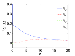
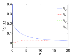
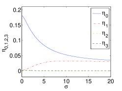
Figure 1: (Color online) The overlap integrals $\eta_{0}$, $\eta_{1}$, $\eta_{2}$ and $\eta_{3}$ as functions of width $\sigma$ of the kernels of the following types: Gaussian (left), exponential (middle), and Lorentzian (right), as defined in Eqs. (4)-(6).

Thus, with $\sigma<\sigma_{b}$, all integrals $\eta_{1,2,3}$ are omitted, and only $\eta_{0}$ is retained. Then, the projection of Eq. (8) onto the two-mode set, $\varphi_{L,R}$, leads to the following ODE system:

$$i\dot{c}_{L} =(\Omega-\mu)c_{L}-\omega c_{R}+s\eta_{0}|c_{L}|^{2}c_{L},$$ (10)

$$i\dot{c}_{R} =(\Omega-\mu)c_{R}-\omega c_{L}+s\eta_{0}|c_{R}|^{2}c_{R}.$$

We then introduce the Madelung representation, $c_{L,R}=\rho_{L,R}e^{i\theta_{L,R}}$ with real time-dependent $\rho_{L,R}$ and $\theta_{L,R}$, and derive from Eq. (10) a set of equations for $\rho_{L,R}$ and $\theta_{L,R}$:

$$\left\{\begin{aligned} \dot{\rho}_{L}&=\omega\rho_{R}\sin{\theta}\\ \dot{\theta}_{L}&=(\mu-\Omega)+\omega\frac{\rho_{R}}{\rho_{L}}\cos{\theta}-s\eta_{0}\rho_{L}^{2}\\ \end{aligned}\right.$$ (11)

where $\theta\equiv\theta_{L}-\theta_{R}$ is the relative phase between the two modes, and the equations for $\rho_{R}$ and $\theta_{R}$ are obtained by interchanging subscripts $L$ and $R$, and $\theta$ with $-\theta$, in Eq. (11) directly. We focus on steady solutions to this system, i.e. $\dot{\rho}_{L,R}=\dot{\theta}_{L,R}=0$. Then, for solutions with nonzero amplitudes, $\theta$ may only take values $0$ or $\pi$, which correspond, respectively, to equal or opposite signs of real stationary solutions for $c_{L}$ and $c_{R}$. Through a straightforward algebra, three stationary solutions are thus found: the symmetric solution, with $\theta=0$ and $\rho_{L,R}^{2}=(\mu-\omega_{0})/s\eta_{0}$, existing when $\mu>\omega_{0}$ ($\mu<\omega_{0}$) for $s=1$ ($s=-1$), i.e., for the repulsive (attractive) long-range interactions; the antisymmetric solution, with $\theta=\pi$ and $\rho_{L,R}^{2}=(\mu-\omega_{1})/s\eta_{0}$, existing when $\mu>\omega_{1}$ ($\mu<\omega_{1}$) for $s=1$ ($s=-1$); and an asymmetric solution, with $\rho_{L,R}^{2}=(s(\mu-\Omega)\pm\sqrt{(\mu-\Omega)^{2}-4\omega^{2}})/2\eta_{0}$. As we assume $\eta_{0}>0$, for the repulsive case ($s=1$) the asymmetric state exists only if $\theta=\pi$, i.e., it bifurcates from the antisymmetric solution when $\mu>\Omega+2\omega$. On the contrary, in the attractive case, it emerges from the symmetric state ($\theta=0$) when $\mu<\Omega-2\omega$. These conclusions agree with the general principles of the SSB theory, according to which the attractive/repulsive nonlinearity breaks the symmetry/anti-symmetry of solutions with equal numbers of particles in the two wells Bergeman_2mode ; todd ; theo ; shliz .

Next, we consider the other situation, in which both $\eta_{0}$ and $\eta_{1}$ are taken into consideration, while the other two are neglected (i.e., $\sigma\geq\sigma_{b}$). In this case, projecting Eq. (8) onto $\varphi_{L,R}$ results in the following system:

$$i\dot{c}_{L} =(\Omega-\mu)c_{L}-\omega c_{R}+sc_{L}(|c_{L}|^{2}\eta_{0}+|c_{R}|^{2}\eta_{1}),$$ (12)

$$i\dot{c}_{R} =(\Omega-\mu)c_{R}-\omega c_{L}+sc_{R}(|c_{R}|^{2}\eta_{0}+|c_{L}|^{2}\eta_{1}).$$

In terms of the Madelung representation, we transform Eqs. (12) into

$$\left\{\begin{aligned} \dot{\rho}_{L}&=\omega\rho_{R}\sin{\theta}\\ \dot{\theta}_{L}&=(\mu-\Omega)+\omega\frac{\rho_{R}}{\rho_{L}}\cos{\theta}-s\eta_{0}\rho_{L}^{2}-s\eta_{1}\rho_{R}^{2},\end{aligned}\right.$$ (13)

with the equations for $\rho_{R}$ and $\theta_{R}$ produced by swapping subscripts $L$ and $R$, and $\theta$ with $-\theta$, as before. In this case, a set of three stationary states are again obtained: the symmetric one, $\theta=0$ and $\rho_{L,R}^{2}=(\mu-\omega_{0})/s(\eta_{0}+\eta_{1})$; the antisymmetric state, $\theta=\pi$ and $\rho_{L,R}^{2}=(\mu-\omega_{1})/s(\eta_{0}+\eta_{1})$. Finally, the asymmetric state, $\theta=\pi$ ($\theta=0$) for $s=1$ ($s=-1$) and $\rho_{L,R}^{2}=((\mu-\Omega)/s\eta_{0}\pm\sqrt{(\mu-\Omega)^{2}/\eta_{0}^{2}-4\omega^{2}/\Delta\eta^{2}})/2$, where $\Delta\eta=\eta_{0}-\eta_{1}>0$ for the kernels we consider, exists at $\mu>\Omega+2\omega\eta_{0}/\Delta\eta$ ($\mu<\Omega-2\omega\eta_{0}/\Delta\eta$) for $s=1$ ($s=-1$). The value of $\mu$ at which the SSB bifurcation happens is tagged as $\mu^{\mathrm{cr}}$. Since $\eta_{0}/\Delta\eta$ is an increasing function of $\sigma$, the value of $\mu^{\mathrm{cr}}$ increases (decreases) as $\sigma$ grows for $s=1$ ($s=-1$).

The two-mode approximation is a powerful means for identifying different steady states of the underlying problem. The solutions found above are also used as initial conditions in solving the full NLS equation (1), as reported in section III.

II.2 The bifurcation analysis

The two-mode approximation strongly facilitates the qualitative analysis of the SSB bifurcation, as well as exploring the system’s dynamics. To proceed, we define the population imbalance between the two wells,

$$z=(N_{L}-N_{R})/N=(|c_{L}|^{2}-|c_{R}|^{2})/N,$$ (14)

where $N_{L,R}=|c_{L,R}|^{2}\equiv\rho_{L,R}^{2}$, hence the total norm is $N=N_{L}+N_{R}$. Together with the relative phase, $\theta=\theta_{L}-\theta_{R}$, we eventually derive the following dynamical equations:

$$\left\{\begin{aligned} \dot{z}&=2\omega\sqrt{1-z^{2}}\sin{\theta}\\ \dot{\theta}&=-\frac{2\omega z\cos{\theta}}{\sqrt{1-z^{2}}}-s\eta Nz.\end{aligned}\right.$$ (15)

This form of the equations is relevant for both cases, when only $\eta_{0}$ or both $\eta_{0}$ and $\eta_{1}$ dominate, as discussed before. Note that $\eta$ stands for $\eta_{0}$ in the former case, and for $\Delta\eta$ in the latter one. Equations (15) take the Hamiltonian form,

$$\left\{\begin{aligned} \dot{z}&=&\>-\frac{\partial\mathcal{H}}{\partial\theta},\\ \dot{\theta}&=&\>\frac{\partial\mathcal{H}}{\partial z},\\ \end{aligned}\right.$$ (16)

with Hamiltonian

$$\mathcal{H}=2\omega\sqrt{1-z^{2}}\cos{\theta}-\frac{1}{2}s\eta Nz^{2}.$$ (17)

Equations (15) possess the stationary solutions, $(z_{1},\theta_{1})$ and $(z_{2},\theta_{2})$, with $z_{1}=z_{2}=0$, $\theta_{1}=0$, $\theta_{2}=\pi$, which represent the symmetric and the antisymmetric solutions, respectively. Besides that, the asymmetric stationary solutions may exist when $N\geq N^{\mathrm{cr}}$, with $N^{\mathrm{cr}}=|2\omega/\eta|$, taking the form of

$$\theta=\pi\;(\theta=0),\quad z^{2}=1-\frac{4\omega^{2}}{\eta^{2}N^{2}},$$ (18)

for $s=1$ ($s=-1$). The asymmetric solution emerges from the antisymmetric (symmetric) one through a pitchfork bifurcation, in the case of the defocusing (focusing) nonlinearity. Since $\eta=\eta_{0}$ for $\sigma<\sigma_{b}$ and $\eta=\eta_{0}-\eta_{1}$ for $\sigma>\sigma_{b}$, Fig. 1 suggests that $\eta$ is, generally, a decreasing function of $\sigma$, and consequently $N^{\mathrm{cr}}$ is increasing with respect to $\sigma$. This way, the bifurcation takes place at larger value of $N$ when the the nonlocality range is wider, which is consistent with the conclusion concerning $\mu^{\mathrm{cr}}$.

Next, from Eq. (15) we derive the equation of motion,

$$\ddot{z}=-4\omega^{2}z+|\eta|Nz\sqrt{4\omega^{2}-4\omega^{2}z^{2}-\dot{z}^{2}},$$ (19)

which leads to the system

$$\left\{\begin{aligned} \dot{z}&=p,\\ \dot{p}&=-4\omega^{2}z+|\eta|Nz\sqrt{4\omega^{2}-4\omega^{2}z^{2}-p^{2}}.\end{aligned}\right.$$ (20)

When $N<N^{\mathrm{cr}}$, there is a unique stationary solution, $p=z=0$, which is a fixed point of the center type. When $N>N^{\mathrm{cr}}$, the origin, $(0,0)$, becomes a saddle, with another pair of fixed points (centers), $p=0$, $z=\pm\sqrt{1-\dfrac{4\omega^{2}}{|\eta|^{2}N^{2}}}$, representing the asymmetric solutions. Figure 2 shows the phase space of system (20), along with the linearization near the fixed points for the example of the Gaussian kernel with $\sigma=5.0$ and $N=0.5$, in which case $N^{\mathrm{cr}}=0.33$.

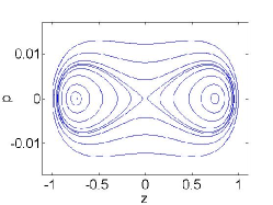
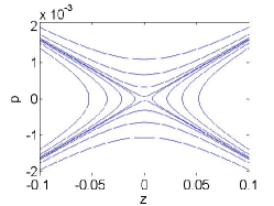
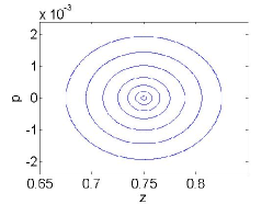
Figure 2: (Color online) Phase diagrams in the Gaussian-kernel model with with $\sigma=5.0$ and $N=0.5$, in which case $N^{\mathrm{cr}}=0.33$. The left panel is obtained from complete system (20), displaying three fixed points, $(0,0)$ and $(\pm 0.7498,0)$. The middle and right panels are the phase planes of the linearized system near fixed points $(0,0)$ (middle) and $(0.7498,0)$ (right).

III Numerical approach

We first consider the repulsive interaction case ($s=1$). Branches of stationary solutions to the full partial differential equation (1) are explored for all three kernels defined in Eqs. (4)-(6) with various values of parameter $\sigma$. The results are plotted in Figs. 3 - 6, where the solutions are expressed in terms of $N$, the number of atoms, as a function of the chemical potential $\mu$. The stationary solutions are sought by employing a fixed-point Newton-Raphson iteration onto a finite difference scheme with $\Delta x=0.1$ and using the continuation of the solutions with respect to $\mu$. The linear stability of each solution $\psi_{0}$, is analyzed by considering the standard linearization around it in the form $\psi(x,t)=\psi_{0}+\varepsilon[a(x)\mathrm{e}^{\lambda t}+b^{*}(x)\mathrm{e}^{\lambda^{*}t}]$. The relevant linear eigenvalue problem is written as

$$\begin{pmatrix}L_{1}&L_{2}\\ -L^{*}_{2}&-L^{*}_{1}\end{pmatrix}=i\lambda\begin{pmatrix}a\\ b\end{pmatrix},$$ (21)

where operators $L_{1}$, $L_{2}$ are defined as

$$L_{1}\phi =\left[-\frac{1}{2}\partial^{2}_{x}+V-\mu+s\int_{-\infty}^{\infty}K\,(x-x^{\prime})|\,\psi_{0}(x^{\prime})|^{2}\,dx^{\prime}\,\right]\,\phi+s\int_{-\infty}^{\infty}K\,(x-x^{\prime})\psi_{0}(x^{\prime})\psi^{*}_{0}(x^{\prime})\phi(x^{\prime})\,dx^{\prime},$$ (22)

$$L_{2}\phi =s\int_{-\infty}^{\infty}K\,(x-x^{\prime})\psi_{0}(x^{\prime})\psi^{*}_{0}(x^{\prime})\phi(x^{\prime})\,dx^{\prime}$$

for any function $\phi$. The stationary state is called unstable if there exist any eigenvalues $\lambda$ with $\Re(\lambda)\neq 0$, otherwise it is stable (i.e. all corresponding eigenvalues are purely imaginary).

We present the results of Gaussian kernel in detail as an example. In each panel (Fig. 3), the solid blue line with highest value of $N$ for any $\mu$ among the three branches is the symmetric stationary solution; the continuation of it to the linear limit ($N\rightarrow 0$) shows that it starts from $\mu=\omega_{0}$ (the eigenvalue associated to the ground mode of the underlying linear system), and it is stable for any $\mu$. The branch with a part of it denoted by dashed red line is the antisymmetric solution, arising from the linear limit at $\mu=\omega_{1}$, corresponding to the first excited state. It starts as a stable state from the linear mode (denoted by solid blue line) and, as $\mu$ increases, after some critical point $\mu^{\mathrm{cr}}$, it is destabilized due to the emergence of the asymmetric branch through a supercritical pitchfork; notice that the asymmetric branch remains stable after it occurs. This bifurcation was predicted by the two-mode analysis in the previous section.

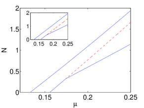
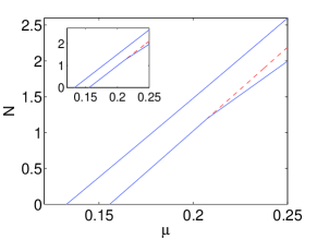
Figure 3: (Color online) The normalized norm, $N$, of the numerically found stationary solutions of the underlying GP equation with the Gaussian kernel, for the case of repulsive interaction ($s=1$), as a function of chemical potential $\mu$. The four panels correspond to cases with different values of $\sigma$, viz., $\sigma=0.1$ (top left), $\sigma=1$ (top right), $\sigma=5$ (bottom left), and, finally, $\sigma=10$ (bottom right). The stationary solutions predicted by the two-mode approximation for each case are shown in the small plot in the top left corner of each panel. The blue solid lines and red dashed lines denote stable and unstable solutions, respectively.

The four panels of Fig. 3 are the bifurcation diagrams of the model with the Gaussian kernel, for $\sigma=0.1,1,5$ and $10$. The main parts of the panels display the numerically found solutions of the full system, while the small plot in each panel shows the corresponding analytical solutions predicted by the two-mode approximation, as obtained in Section II. The numerical and analytical branches of the solutions demonstrate good agreement in all the four cases. Recall that we have obtained the critical values at which the bifurcation takes place, $\mu^{\mathrm{cr}}$ (or equivalently $N^{\mathrm{cr}}$), in an analytical form. As for the Gaussian kernel (with the chosen border at $\sigma_{b}=2.96$), $\sigma=0.1$ and $\sigma=1$ are categorized as belonging to the first case, with solely $\eta_{0}$ taken into account, among all the overlap integrals. The analytically predicted value is $\mu^{\mathrm{cr}}=0.1671$ (since $\mu^{\mathrm{cr}}=\Omega+2\omega$), while its numerically found counterpart is $\mu^{\mathrm{cr}}=0.1684$ for both $\sigma=0.1$ and $1$. On the other hand, $\sigma=5$ and $\sigma=10$ pertain to the the second case, in which both $\eta_{0}$ and $\eta_{1}$ are kept. In this case, the analytical prediction is $\mu^{\mathrm{cr}}=\Omega+2\omega\eta_{0}/\Delta\eta$, which depends on $\eta_{0,1}$ and thus varies for different values of $\sigma$. The predicted values of $\mu^{\mathrm{cr}}$ is $0.1757$ and $0.2120$, for $\sigma=5$ and $10$, respectively, while the respective numerical values are $\mu^{\mathrm{cr}}=0.1745$ and $0.2075$. Despite a small discrepancy between the two groups of the values (numerical versus analytical), the analytical results still succeed in predicting the trend of the behavior of $\mu^{\mathrm{cr}}$, viz., $\mu^{\mathrm{cr}}$ increases with the growth of $\sigma$, or, in other words, the SSB bifurcation takes place at higher values of $N^{\mathrm{cr}}$, as shown in Fig. 4.

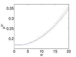
Figure 4: (Color online) The critical value of the chemical potential, $\mu^{\mathrm{cr}}$, at which the supercritical pitchfork bifurcation takes place in the case of the self-repulsive nonlinearity with the Gaussian kernel, as a function of $\sigma$. The blue solid line and the red dashed-dotted line denote the numerically obtained values and their counterparts predicted by the two-mode approximation, respectively. Note that there is a small jump at $\sigma=2.96$ on the dashed-dotted line, due to the definition if the border between the two situations [described by Eqs. (10) and (12), respectively] in the two-mode analysis.

Next we consider cases with the long-range interaction based on the other two kernels, viz., the exponential and Lorentzian ones, given by Eq. (5) and (6), respectively. The corresponding bifurcation diagrams, similar to the case of the Gaussian kernel, are presented in Fig. 5 and Fig. 6, with the same notations as adopted above.

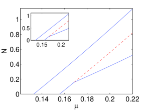
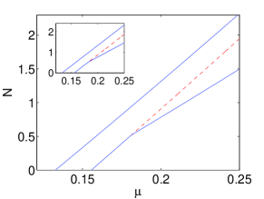
Figure 5: (Figure online) Norm $N$ of the numerically found solutions and their counterparts predicted by the two-mode approximation (shown in the corners) for the case of the self-repulsive nonlinearity with the exponential kernel, as a function of $\mu$. Here and in the next figure, the value of $\sigma$ is chosen as $\sigma=1$ (left), $\sigma=5$ (right), and the notation is the same as in Fig. 3.

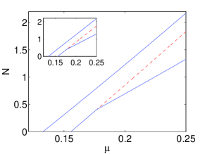
Figure 6: (Color online) The norm of the numerical and approximate analytical solutions for the case of the self-repulsive nonlinearity with the Lorentzian kernel, as a function of $\mu$.

Lastly, we also briefly discuss the self-attractive case, with $s=-1$ in Eq. (1). Two examples are selected, using the Gaussian kernel with $\sigma=1$ and $5$, to help illustrating the similarities and differences with the self-repulsive case. The complete bifurcation diagrams are plotted, for this case, in Fig. 7, with the notation similar to that introduced above.

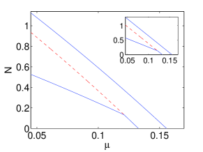
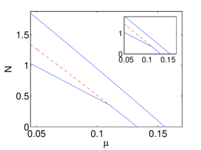
Figure 7: (Color online) Norm $N$ of the numerical solutions, together with their analytical counterparts (shown in the small plots on the top right corners), for the case of the self-attractive nonlinearity ($s=-1$), as a function of $\mu$. The Gaussian kernel is taken, with $\sigma=1$ (left) and $\sigma=5$ (right). The notation is the same as in Fig. 3.

In this case, the two branches arise from the linear modes at $\mu=\omega_{0}$ and $\omega_{1}$, pertaining to the symmetric and antisymmetric stationary solutions, which exist for $\mu<\omega_{0}$ or $\mu<\omega_{1}$, respectively. This time, the supercritical SSB pitchfork bifurcation occurs on the symmetric branch, leading to the emergence of the asymmetric state. The pitchfork is found at $\mu^{\mathrm{cr}}=0.1213$ and $0.1128$ for $\sigma=1$ and $5$ respectively, in good agreement with the critical values predicted by the two-mode approximation, which are $0.1212$ and $0.1104$. In each panel of Fig. 7, the diagram produced by the two-mode approximation, corresponding to its numerical counterpart, is displayed in the top right corner, exhibiting a very good agreement between the two.

IV Competing short- and long-range interactions

In this section, we consider a model illustrating effects of the competition of the long-range interactions with local ones, based on the following GP equation,

$$i\partial_{t}\psi+\mu\psi=L\psi+s\left[\int_{-\infty}^{\infty}K\,(x-x^{\prime})|\,\psi(x^{\prime})|^{2}\,dx^{\prime}\,\right]\,\psi+g|\psi|^{2}\psi,$$ (23)

where coefficient $g$ accounts for the contact nonlinearity. The interactions are fully attractive or repulsive if $s$ and $g$ are both negative or positive, respectively. However, in such cases the results turn out to be similar to those reported above for the nonlocal nonlinearity. A more interesting case arises for $sg<0$, i.e., for the competing interactions. Effects of the competition on 1D solitons were recently studied in detail in Ref. us .

We use the analysis presented in the previous section as a starting point for our considerations here. Thus, we fix the long-range interaction coefficient $s=\pm 1$, and then vary the local interaction coefficient, $g$ from $0$ to $-1$ ($g<0$ implies the local attraction), using Gaussian kernel (4) with $\sigma=5$ and $s=1$ as a case example. As the attractive local interactions grow stronger, interesting phenomena emerge in the development of the corresponding bifurcation diagram, as is shown in Fig. 8.

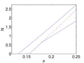
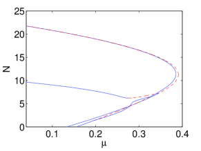
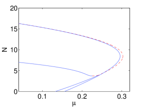
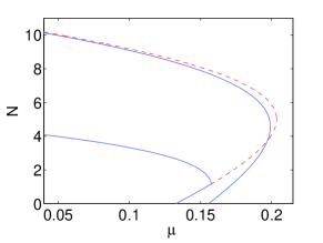
Figure 8: (Color online) Norm $N$ of the numerically found solutions in the case of the competing interactions for Gaussian kernel (4) with $\sigma=5$, as a function of $\mu$. The coefficient of the long-range interactions is $s=1$, while the local-interaction coefficient is $g=-0.2$ (top left), $-0.3$ (top right), $-0.35$ (bottom left) and $-0.45$ (bottom right). The notation is the same as in Fig. 3.

When $g$ is close to zero, the three branches of stationary states are similar to those in the case of pure long-range interactions, as shown in the bottom left panel of Fig. 3. An example for $g=-0.2$ is presented in the top left panel of Fig. 8, where the norm $N$ of each branch is larger at any value of $\mu$, in comparison to the case of $g=0$. Also, the bifurcation takes place at a larger critical value, $\mu^{\mathrm{cr}}=0.1805$.

As $g$ grows more negative, we notice that the symmetric and the antisymmetric branches, while monotonically increasing with $\mu$ at small values of $N$, switch to become monotonically decreasing functions of $\mu$ at a large value of $N$. Simultaneously, we observe the bifurcation of two asymmetric states, each from a different branch. While it is commonly known that attractive and repulsive interactions favor bifurcations from symmetric and anti-symmetric branches, respectively, here we encounter the first (to our knowledge) example that features bifurcations from both branches. This unusual situation extends up to $g=-0.32$. The complete bifurcation diagram is displayed in the top right panel of Fig. 8, for the case of $g=-0.3$. In this case, the symmetric and antisymmetric branches arise, as usual, from their linear limits at $\mu=\omega_{0}$ and $\mu=\omega_{1}$, respectively. A supercritical pitchfork bifurcation occurring (as before) on the antisymmetric branch gives rise to an asymmetric state at $\mu=-0.195$, destabilizing the antisymmetric one. What is, however, different here is that this asymmetric state “survives” only within a narrow parametric interval before it merges back into the antisymmetric branch through another subcritical (“symmetry-restoring”) pitchfork at $\mu=0.3263$. This bifurcation loop is reminiscent of that reported previously for two-component solitons in local 1D and 2D models with competing self-focusing cubic and self-defocusing quintic nonlinearities loop . For higher $\mu$, another asymmetric branch arises from the symmetric one through a subcritical pitchfork at $\mu=0.3465$; it is especially important to highlight that this pitchfork, which destabilizes the symmetric branch, is a subcritical one, hence the asymmetric state is unstable too. It is observed that, after its emergence, the norm of the asymmetric branch decreases as $\mu$ decreases ($dN/d\mu>0$), before starting to rise at the fold point at $\mu=0.2768$, featuring $dN/d\mu<0$ after that. The stability of the state changes at the turning point, which is in agreement with the well-known Vakhitov-Kolokolov (VK) criterion vk , according to which the slope of the branch determines its stability. In Fig. 9, a blowup provides a clearer view of these bifurcations.

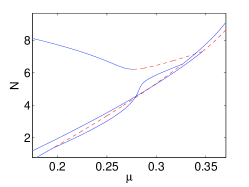
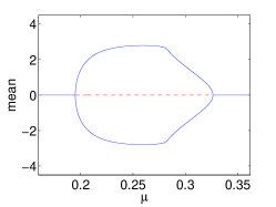
Figure 9: (Color online) The left panel: a segment of the top right panel in Fig. 8, for $g=-0.35$, clarifies details of the bifurcation picture. The right panel: the asymmetry-measuring intergal characteristic, $\int_{-\infty}^{+\infty}x|\psi|^{2}dx$, for the antisymmetric solution and the asymmetric one arising from it, as a function of $\mu$, in the same case as in the left panel. The loop illustrating the asymmetric solution emerging from (through the symmetry-breaking supercritical pitchfork) and merging back (through the symmetry-restoring subcritical pitchfork) into the antisymmetric branch. The notation is the same as in Fig. 3.

The symmetric and the antisymmetric branches continue to increase their norms with the growth of $\mu$, each of them featuring its own turning point, at $\mu=0.391$ and $\mu=0.3853$ respectively, and change their monotonicity thereafter. However, this change on the antisymmetric branch is not accompanied by a stability change. To demonstrate that this is not an exception to the VK criterion, we define the linearization operators,

$$L_{+} =L_{1}+L_{2}+3g|\psi|^{2},$$ (24)

$$L_{-} =L_{1}-L_{2}+g|\psi|^{2},$$

using notation $L_{1,2}$ defined in Eq. (22). It is known from Ref. grill that the instability arises, when the slope condition of the VK criterion is violated, if $|n(L_{+})-n(L_{-})|=1$, $n$ standing for the number of negative eigenvalues of each operator. The state under consideration is generically unstable if $|n(L_{+})-n(L_{-})|>1$. In our case, the antisymmetric branch has $n(L_{-})\equiv 1$ (due to its single-zero-crossing configuration profile, which is a zero mode of $L_{-}$). Meanwhile, $n(L_{+})=1$ is true before the branch turns to the left, and consequently $|n(L_{+})-n(L_{-})|=0$. Hence, even though the slope condition is violated ($dN/d\mu>0$), the relevant theorem suggests that the VK criterion does not actually apply here (and no stability change occurs). After the turning point, the stability is expected since $n(L_{+})=2$, and the slope condition is satisfied, which is in accordance with our observations.

Next, as the local interactions continue to grow stronger, another regime is explored, as shown in the bottom left panel of Fig. 8, with $g=-0.35$ as an example. In this case, the phenomenology of the symmetric branch is similar to that in the previous situation; however, the two sequential bifurcations taking place on the antisymmetric branch no longer arise. Hence, the entire antisymmetric branch remains dynamically stable. The asymmetric branch still emerges from the symmetric one through a subcritical pitchfork, and later becomes stable past the fold point due to the change of slope, in accordance with the VK criterion.

The above regime persists until $g=-0.38$. After that, the pitchfork bifurcation occurring on the symmetric branch switches from subcritical to supercritical, leading to the emergence of a stable asymmetric branch, as shown in the last panel of Fig. 8. This shape of the bifurcation diagram, consisting of the three branches, persists as far as $g$ decreases to $-1$. Note that during this process, the turning points of the symmetric and antisymmetric branches keep getting lower (with respect to $N$), finally leading to a situation where the turning points do not exist, and the two branches immediately go left starting from their linear limits, i.e., the symmetric and the antisymmetric solutions only exist for $\mu<\omega_{0},\;\omega_{1}$ when $g<-0.69,\;-0.6$, respectively.

V Conclusions and future challenges

In this work, we have presented a systematic study of the interplay between the long-range nonlinear interactions (of either sign, repulsive or attractive) and linear double-well potential (DWP) in the 1D setting. The two-mode approximation has been developed, that accounts for the nonlocality but retains the structure similar to that established before in the case of the contact interaction. This conclusion demonstrates that the fundamental phenomenology of the spontaneous symmetry breaking (SSB) in the DWP persists in the presence of the longer-range interactions, although the critical properties themselves (e.g., the critical values of the chemical potential and norm), at which the SSB bifurcation occurs, giving rise to the asymmetric steady states, are sensitive to the precise interaction range. In particular, our analysis has revealed a monotonous increase of the critical values as a function of the interaction range, in the case of the self-repulsion. A considerably more elaborate phenomenology was revealed by the analysis in the context of competing long- and short-range interactions. In that case, a delicate interplay between the strengths of the nonlocal repulsion and local attraction gives rise, in addition to predominantly attractive and predominantly repulsive regimes, to mixed ones with complex bifurcation phenomena. On the one hand, symmetry-breaking effects were shown to arise from each of the relevant solution branches; in some cases, they are accompanied by reverse bifurcations, to form closed loops. On the other hand, some of the previously studied supercritical bifurcations, such as the one occurring on the symmetric branch, could become subcritical, being subsequently coupled to additional fold bifurcations. All of these effects are absent, to our knowledge, in models with a single cubic nonlinear term, being consequences of the competition.

These results may be a motivation for studies in a number of future directions. In particular, it would be relevant to consider the generalizations of the DWP setting to higher dimensions, such as, the four-well configuration, which was recently demonstrated to yield a much richer phenomenology in the case of the contact interactions chenyu2d . In the same connection, it is relevant to note that the few-mode approach, used in this work for the consideration of the existence and stability of the symmetric, antisymmetric, and asymmetric states, as functions of the interaction strength, may be applied to other structures, such as multi-dimensional bright Pedri05 , dark sann and vortex Krolik solitons, especially in cases where such structures are stabilized by nonlocal nonlinearities. A natural objective of such an analysis may be to unravel effects of the interaction range on structural stability of nonlinear waveforms. Such studies are presently in progress and will be reported elsewhere.

- (1) L. P. Pitaevskii, S. Stringari, Bose-Einstein Condensation (Oxford University Press, Oxford, 2003).
- (2) C. J. Pethick and H. Smith, Bose-Einstein condensation in dilute gases (Cambridge University Press, Cambridge, 2002).
- (3) P. G. Kevrekidis, D. J. Frantzeskakis, and R. Carretero-González (eds.), Emergent nonlinear phenomena in Bose-Einstein condensates. Theory and experiment (Springer-Verlag, Berlin, 2008).
- (4) Yu. S. Kivshar and G. P. Agrawal, Optical solitons: from fibers to photonic crystals (Academic Press, San Diego, 2003).
- (5) C. Sulem and P. L. Sulem, The Nonlinear Schrödinger Equation (Springer-Verlag, New York, 1999).
- (6) O. Morsch and M. Oberthaler, Rev. Mod. Phys. 78, 179 (2006).
- (7) M. Albiez, R. Gati, J. Fölling, S. Hunsmann, M. Cristiani, and M. K. Oberthaler, Phys. Rev. Lett. 95, 010402 (2005).
- (8) S. Raghavan, A. Smerzi, S. Fantoni, and S. R. Shenoy, Phys. Rev. A 59, 620 (1999); S. Raghavan, A. Smerzi, and V. M. Kenkre, Phys. Rev. A 60, R1787 (1999); A. Smerzi and S. Raghavan, Phys. Rev. A 61, 063601 (2000).
- (9) E. A. Ostrovskaya, Yu. S. Kivshar, M. Lisak, B. Hall, F. Cattani, and D. Anderson, Phys. Rev. A 61, 031601(R) (2000).
- (10) K. W. Mahmud, J. N. Kutz, and W. P. Reinhardt, Phys. Rev. A 66, 063607 (2002).
- (11) V. S. Shchesnovich, B. A. Malomed, and R. A. Kraenkel, Physica D 188, 213 (2004).
- (12) D. Ananikian and T. Bergeman, Phys. Rev. A 73, 013604 (2006).
- (13) P. Ziń, E. Infeld, M. Matuszewski, G. Rowlands, and M. Trippenbach, Phys. Rev. A 73, 022105 (2006).
- (14) T. Kapitula and P. G. Kevrekidis, Nonlinearity 18, 2491 (2005).
- (15) G. Theocharis, P. G. Kevrekidis, D. J. Frantzeskakis, and P. Schmelcher, Phys. Rev. E 74, 056608 (2006).
- (16) D. R. Dounas-Frazer, A. M. Hermundstad, and L. D. Carr, Phys. Rev. Lett. 99, 200402 (2007).
- (17) T. Mayteevarunyoo, B. A. Malomed, and G. Dong. Phys. Rev. A 78, 053601 (2008).
- (18) C. Paré and M. Florjańczyk, Phys. Rev. A 41, 6287 (1990); A. I. Maimistov, Kvant. Elektron. 18, 758 (1991) [In Russian; English translation: Sov. J. Quantum Electron. 21, 687; W. Snyder, D. J. Mitchell, L. Poladian, D. R. Rowland, and Y. Chen, J. Opt. Soc. Am. B 8, 2102 (1991); P. L. Chu, B. A. Malomed, and G. D. Peng, J. Opt. Soc. Am. B 10, 1379 (1993); N. Akhmediev, and A. Ankiewicz, Phys. Rev. Lett. 70, 2395 (1993); B. A. Malomed, I. Skinner, P. L. Chu, and G. D. Peng, Phys. Rev. E 53, 4084 (1996).
- (19) C. Cambournac, T. Sylvestre, H. Maillotte , B. Vanderlinden, P. Kockaert, Ph. Emplit, and M. Haelterman, Phys. Rev. Lett. 89, 083901 (2002).
- (20) P. G. Kevrekidis, Z. Chen, B. A. Malomed, D. J. Frantzeskakis, and M. I. Weinstein, Phys. Lett. A 340, 275 (2005).
- (21) A. Griesmaier, J. Werner, S. Hensler, J. Stuhler, and T. Pfau, Phys. Rev. Lett. 94, 160401 (2005); J. Stuhler, A. Griesmaier, T. Koch, M. Fattori, T. Pfau, S. Giovanazzi, P. Pedri, and L. Santos, ibid. 95, 150406 (2005); J. Werner, A. Griesmaier, S. Hensler, J. Stuhler, and T. Pfau, ibid. 94, 183201 (2005); A. Griesmaier, J. Stuhler, T. Koch, M. Fattori, T. Pfau, and S. Giovanazzi, ibid. 97, 250402 (2006); A. Griesmaier, J. Phys. B: At. Mol. Opt. Phys. 40, R91 (2007); T. Lahaye, T. Koch, B. Fröhlich, M. Fattori, J. Metz, A. Griesmaier, S. Giovanazzi, and T. Pfau, Nature (London) 448, 672 (2007).
- (22) T. Lahaye, C. Menotti, L. Santos, M. Lewenstein and T. Pfau, Rep. Progr. Phys. 72, 126401 (2009).
- (23) T. Köhler, K. Góral, and P. S. Julienne, Rev. Mod. Phys. 78, 1311 (2006); J. Sage, S. Sainis, T. Bergeman, and D. DeMille, Phys. Rev. Lett. 94, 203001 (2005); C. Ospelkaus, L. Humbert, P. Ernst, K. Sengstock, and K. Bongs, ibid. 97, 120402 (2006); J. Deiglmayr, A. Grochola, M. Repp, K. Mörtlbauer, C. Glück, J. Lange, O. Dulieu, R. Wester, and M. Weidemüller, ibid. 101, 133004 (2008); F. Lang, K. Winkler, C. Strauss, R. Grimm, and J. H. Denschlag, ibid. 101, 133005 (2008).
- (24) M. Marinescu and L. You, Phys. Rev. Lett. 81, 4596 (1998); S. Giovanazzi, D. O’Dell, and G. Kurizki, Phys. Rev. Lett. 88, 130402 (2002); I. E. Mazets, D. H. J. O’Dell, G. Kurizki, N. Davidson, and W. P. Schleich, J. Phys. B 37, S155 (2004); R. Löw, R. Gati, J. Stuhler and T. Pfau, Europhys. Lett. 71, 214 (2005).
- (25) P. Pedri and L. Santos, Phys. Rev. Lett. 95, 200404 (2005); R. Nath, P. Pedri, and L. Santos, Phys. Rev. A 76, 013606 (2007); I. Tikhonenkov, B. A. Malomed, and A. Vardi, Phys. Rev. A 78, 043614 (2008).
- (26) I. Tikhonenkov, B. A. Malomed, and A. Vardi, Phys. Rev. Lett. 100, 090406 (2008).
- (27) G. Gligorić, A. Maluckov, M. Stepić, Lj. Hadžievski, and B. A. Malomed, Phys. Rev. A 81, 013633 (2010); J. Phys. B: At. Mol. Opt. Phys. 43, 055303 (2010).
- (28) S. Sinha and L. Santos, Phys. Rev. Lett. 99, 140406 (2007).
- (29) J. Cuevas, B. A. Malomed, P. G. Kevrekidis and D. J. Frantzeskakis, Phys. Rev. A 79, 053608 (2009).
- (30) B. B. Baizakov, F. Kh. Abdullaev, B. A. Malomed, and M. Salerno, J. Phys. B: At. Mol. Opt. Phys. 42, 175302 (2009).
- (31) D. Briedis, D. E. Petersen, D. Edmundson, W. Królikowski, and O. Bang, Opt. Exp. 13, 435 (2005).
- (32) C. Rotschild, O. Cohen, O. Manela, and M. Segev, Phys. Rev. Lett. 95, 213904 (2005).
- (33) B. Xiong, J. Gong, H. Pu, W. Bao, and B. Li, Phys. Rev. A 79, 013626 (2009), M. Asad-uz-Zaman and D. Blume, ibid. 80, 053622 (2009).
- (34) W. Królikowski, O. Bang, J. J. Rasmussen, and J. Wyller, Phys. Rev. E 64, 016612 (2001); O. Bang, W. Królikowski, J. Wyller and J. J. Rasmussen, Phys. Rev. E 66, 046619 (2002); J. Wyller, W. Królikowski, O. Bang and J. J. Rasmussen, Phys. Rev. E 66, 066615 (2002).
- (35) E. W. Kirr, P. G. Kevrekidis, E. Shlizerman and M. I. Weinstein, SIAM J. Math. Anal. 40, 566 (2008).
- (36) A. Sacchetti, Phys. Rev. Lett. 103, 194101 (2009).
- (37) L. Albuch and B. A. Malomed, Mathematics and Computers in Simulation 74, 312 (2007); Z. Birnbaum and B. A. Malomed, Physica D 237, 3252 (2008).
- (38) N. G. Vakhitov, A. A. Kolokolov, Radiophys. Quantum Electron. 16, 783 (1973); Z. Birnbaum and B. A. Malomed, Physica D 237, 3252 (2008).
- (39) M. G. Grillakis, J. Shatah, W. A. Strauss, J. Funct. Anal. 74, 160 (1987)
- (40) C. Wang, G. Theocharis, P. G. Kevrekidis, N. Whitaker, K. J. H. Law, D. J. Frantzeskakis, and B. A. Malomed Phys. Rev. E 80, 046611 (2009)
- (41) R. Nath, P. Pedri, and L. Santos Phys. Rev. Lett. 101, 210402 (2008)