Error Analysis of Approximated PCRLBs for Nonlinear Dynamics

Abstract

In practical nonlinear filtering, the assessment of achievable filtering performance is important. In this paper, we focus on the problem of efficiently approximate the posterior Cramer-Rao lower bound (CRLB) in a recursive manner. By using Gaussian assumptions, two types of approximations for calculating the CRLB are proposed: An exact model using the state estimate as well as a Taylor-series-expanded model using both of the state estimate and its error covariance, are derived. Moreover, the difference between the two approximated CRLBs is also formulated analytically. By employing the particle filter (PF) and the unscented Kalman filter (UKF) to compute, simulation results reveal that the approximated CRLB using mean-covariance-based model outperforms that using the mean-based exact model. It is also shown that the theoretical difference between the estimated CRLBs can be improved through an improved filtering method.

I Introduction

It is well known that optimal estimators for the nonlinear filtering of the discrete-time dynamic systems is an active area of research and that a large number of suboptimal approximated approaches were developed [1]. It is important to quantify the accuracy of estimates obtained for the design of algorithms such as the interacting multiple models (IMM) where weighted estimates from multiple estimators are simultaneously employed.

During the past thirty years many attempts have been made to theoretically derive the achievable performance of nonlinear filters. Deriving performance bounds are important since such bound serve as indicators to measure system performance, and can be used to determine whether imposed performance requirements are realistic or not.

For dynamical statistical models, a commonly used bound is the CRLB that has been investigated by various researchers: Van Trees [2] presented the batch form of a posterior CRLB for random parameter vectors and a pre-1989 review [3] summarized several lower bounds for nonlinear filtering, which heavily emphasized the continuous time case. Bobrovsky [4] applied CRLB to discrete time problems and Galdos [6] generalized it to the multi-dimensional case. The main shortcoming of these formulations is the batch form of implementation resulting high computational loads. Tichavsky [7] was the first to derive a recursive CRLB for updating the posterior Fisher information matrix (FIM) from one time instance to the next while keeping the FIM constant in size.

Subsequently, CRLB theory was extended to many applications, e.g., introducing the CRLB to multiple target tracking [9], incorporating data association for tracking with the CRLB [10], target detection for the case having a detection probability less than unit [8], etc.

It is well known that the matrices in recursive form of FIM, can only be theoretically determined by the true value of state. Unfortunately, we cannot obtain the true state online in practice, except in some well-designed experiments where true value of the state is given as a prior knowledge. Therefore we naturally focus on how to determine an approximate CRLB by using online state estimates (as opposed to the true state values).

We have mainly two ways to approximate the CRLB [5]: 1) Make full use of the first-two order moments of the state estimate, i.e., expectation and covariance, by incorporating them with the Taylor series expansion of the dynamics. 2) Combine the expectation of the state with the exact dynamic model directly. The first method use both estimates and is rather complex while the second method is considerably simple, but depends heavily on an exact model. The second method is mostly preferred in practice for its simpleness and is sufficient to obtain an usable approximated CRLB.

The following question therefore needs to be addressed: By how much the CRLB employed the two kinds of approximations differ from, and which one is a better approximation to the true CRLB. This is the main motivation of this investigation. In addition, determining the accuracy of the estimated CRLB by using a state estimate, rather than the true state under a recursive framework for a general nonlinear dynamics, has not been addressed previously.

In this paper, we show how the state estimates can be applied to determine the difference between the two estimated CRLBs. By using Monte Carlo simulations, we show that the proposed method achieve a satisfactory approximation, and the accuracy of estimated CRLB can be explicitly improved by increasing the accuracy of filtering.

II Problem Formulation

II-A Nonlinear Dynamical Model

Consider the following discrete-time nonlinear dynamics with additive Gaussian noise:

$${\bf x}_{k+1}={\bf f}_{k}({\bf x}_{k})+{\bf w}_{k},$$ (1)

$${\bf z}_{k}={\bf h}_{k}({\bf x}_{k})+{\bf v}_{k},$$ (2)

where the nonlinear vector-valued functions ${\bf f}_{k}\in\mathbb{R}^{n\times 1}$ and ${\bf h}_{k}\in\mathbb{R}^{m\times 1}$ be used to model the state kinematics and measurement respectively, and generally $n>m$. ${\bf x}_{k}\in\mathbb{R}^{n\times 1}$ is the state vector, ${\bf z}_{k}\in\mathbb{R}^{m\times 1}$ is the measurement vector, ${\bf w}_{k}\in\mathbb{R}^{n\times 1}$ is a zero-mean white Gaussian process noise with known covariance ${\bf Q}_{k}$, and ${\bf v}_{k}\in\mathbb{R}^{m\times 1}$ a zero-mean Gaussian white measurement noise with variance ${\bf R}_{k}$. The initial state ${\bf x}_{0}$ is assumed as a Gaussian distribution with mean ${\bar{\bf x}}_{0}$ and variance ${\bf P}_{0}$. Moreover, a general accepted assumption like $cov({\bf x}_{0},{\bf v}_{k})=0,cov({\bf x}_{0},{\bf w}_{k})=0$.

II-B Posterior CRLB

Let ${\hat{\bf x}}_{k}$ and ${\bf C}_{k}$ denote the unbiased state estimate and its error covariance at time instant $k$. We therefore have

$${\bf C}_{k}=E\!\left[{\tilde{\bf x}}_{k}{\tilde{\bf x}}^{\prime}_{k}\right]\geq{\bf J}_{k}^{-1},$$ (3)

where ${\tilde{\bf x}}_{k}={\bf x}_{k}-{\hat{\bf x}}_{k}$ is the prediction error of state. ${\bf J}_{k}^{-1}$ is the posterior CRLB (PCRLB), defined to be the inverse of FIM, ${\bf J}_{k}$. The superscript $(\cdot)^{\prime}$ in (3) denotes the transpose of a vector or a matrix, and the inequality in (3) means that the difference ${\bf C}_{k}-{\bf J}_{k}^{-1}$ is a positive semidefinite matrix. From [7, 11] we know that the sequential FIM ${\bf J}_{k}$ can be recursively calculated by

$${\bf J}_{k+1}={\bf D}_{k}^{22}-{\bf D}_{k}^{21}({\bf J}_{k}+{\bf D}_{k}^{11})^{-1}{\bf D}_{k}^{12}\quad(k>0),$$ (4)

$${\bf J}_{0}=E\left[-\Delta_{{\bf x}_{0}}^{{\bf x}_{0}}\log p({\bf x}_{0})\right],$$ (5)

$${\bf D}_{k}^{11}=E\left[-\Delta_{{\bf x}_{k}}^{{\bf x}_{k}}\log p({\bf x}_{k+1}|{\bf x}_{k})\right],$$ (6)

$${\bf D}_{k}^{12}=\left({\bf D}_{k}^{21}\right)^{\prime}=E\left[-\Delta_{{\bf x}_{k}}^{{\bf x}_{k+1}}\log p({\bf x}_{k+1}|{\bf x}_{k})\right],$$ (7)

$${\bf D}_{k}^{22}=E\left[-\Delta_{{\bf x}_{k+1}}^{{\bf x}_{k+1}}\log p({\bf x}_{k+1}|{\bf x}_{k})\right]+$$

$$\quad\quad E\left[-\Delta_{{\bf x}_{k+1}}^{{\bf x}_{k+1}}\log p({\bf z}_{k+1}|{\bf x}_{k+1})\right],$$ (8)

here let $\nabla$ and $\Delta$ be operators of the first and second-order partial derivatives, i.e., $\nabla_{\bf x}=\left[\frac{\partial}{\partial x_{1}},\cdots,\frac{\partial}{\partial x_{n}}\right]^{\prime},\Delta_{\bf x}^{\bf y}=\nabla_{\bf x}(\nabla_{\bf y})^{\prime}$. Note that all the above expectations are taken with respect to the joint probability density function (PDF) $p({\bf x}_{0:k+1}|{\bf z}_{1:k+1})$, where ${\bf x}_{0:k+1}$ and ${\bf z}_{1:k+1}$ denote all the states and measurements up to time $k+1$.

III Approximated Gaussian Form (AGF) of Nonlinear Dynamics

According to CRLB theory, the derivatives in (4) should be evaluated at the true value of state ${\bf x}_{k}$. Our final aim is to use the moments of state estimate instead of the true state to calculate the difference between the approximated PCRLBs, thus the FIM matrices (i.e., ${\bf D}_{k}^{11}$, ${\bf D}_{k}^{12}$ and ${\bf D}_{k}^{22}$ should be represented, therefore, the density function $p({\bf x}_{k+1}|{\bf x}_{k})$ and $p({\bf z}_{k+1}|{\bf x}_{k+1})$ from (1) and (2) should be firstly formulated explicitly.

III-A AGF by the First-two Order Moment of State Estimate

Assume that the first and second moment estimation of state ${\bf x}_{k}$ is known and given by ${\hat{\bf x}}_{k}$ and ${\hat{\bf P}_{k}^{\bf f}}=E\left[{\tilde{\bf x}}_{k}{\tilde{\bf x}}^{\prime}_{k}|{\bf z}_{1:k}\right]$, and also assume that the distribution of ${\bf x}_{k+1}$ can be approximated by a Gaussian. We immediately have

$${\bf x}_{k+1}\approx\mathcal{N}\!\left[{\bf x}_{k+1};~{}{\bar{\bf x}}_{k+1},~{}{\bf P}_{k+1}^{\bf x}\right],$$ (9)

where ${\bar{\bf x}}_{k+1}=E\left[{\bf x}_{k+1}|{\bf z}_{1:k}\right]\approx{\hat{\bf f}}_{k}+{\breve{\bf f}}_{k}$, in which ${\hat{\bf f}}_{k}={\bf f}_{k}({\hat{\bf x}}_{k})$, ${\breve{\bf f}}_{k}=\frac{1}{2}\sum_{i=1}^{n}{\bf e}_{i}tr\left[{\hat{\bf S}}_{k,i}^{{\bf f}}{\hat{\bf P}}_{k}^{{\bf f}}\right]$, ${\bf e}_{i}\in\mathbb{R}^{n\times 1}$ denotes the $i$-th unit normal vector in column shape, and $tr[\cdot]$ denotes trace operation. ${\hat{\bf S}}_{k,i}^{\bf f}=\nabla_{{\bf x}_{k}}\left[\nabla_{{\bf x}_{k}}f_{k,i}({\bf x}_{k})\right]^{\prime}$ is the Hessian matrix of $i$-th element $f_{k,i}({\bf x}_{k})$ of the vector-valued function ${\bf f}_{k}({\bf x}_{k})$. Notation ${\hat{\bf F}}_{k}^{\bf f}=\left[\nabla_{{\bf x}_{k}}{\bf f}^{\prime}_{k}({\bf x}_{k})\right]^{\prime}=\left[\partial f_{k,i}({\bf x}_{k})/\partial x_{j}\right]_{n\times n}$ denotes the Jacobian matrix with $n\times n$ dimension, ${\bf P}_{k+1}^{\bf x}={\breve{\bf P}}_{k+1}^{\bf x}+{\bf Q}_{k}$, ${\breve{\bf P}}_{k+1}^{\bf x}={\hat{\bf F}}_{k}^{\bf f}{\hat{\bf P}}_{k}^{\bf f}({\hat{\bf F}}_{k}^{\bf f})^{\prime}+\frac{1}{2}\sum_{i=1}^{n}\sum_{j=1}^{n}{\bf e}_{i}{\bf e}^{\prime}_{j}tr\left[{\hat{\bf S}}_{k,i}^{\bf f}{\hat{\bf P}}_{k}^{\bf f}{\hat{\bf S}}_{k,j}^{\bf f}{\hat{\bf P}}_{k}^{\bf f}\right]$. Similar to (9), the Gaussian form of the measurement ${\bf z}_{k}$ can be approximated by

$${\bf z}_{k}\approx\mathcal{N}\left[{\bf z}_{k};~{}{\bar{\bf z}}_{k},~{}{\bf P}_{k}^{\bf z}\right],$$ (10)

where the expectation ${\bar{\bf z}}_{k}=E\left[{\bf z}_{k}|{\bf x}_{k}\right]\approx{\hat{\bf h}}_{k}+{\breve{\bf h}}_{k}$, the covariance ${\bf P}_{k}^{\bf z}\approx{\bf R}_{k}+{\breve{\bf P}}_{k}^{\bf z}$, in which ${\breve{\bf h}}_{k}=\frac{1}{2}\sum_{i=1}^{m}{\bf e}_{i}tr\left[{\hat{\bf S}}_{k,i}^{\bf h}{\hat{\bf P}}_{k}^{\bf h}\right]$, ${\breve{\bf P}}_{k}^{\bf z}={\hat{\bf F}}_{k}^{\bf h}{\hat{\bf P}}_{k}^{\bf h}({\hat{\bf F}}_{k}^{\bf h})^{\prime}+\frac{1}{2}\sum_{i=1}^{m}\sum_{j=1}^{m}{\bf e}_{i}{\bf e}^{\prime}_{j}tr\left[{\hat{\bf S}}_{k,i}^{\bf h}{\hat{\bf P}}_{k}^{\bf h}{\hat{\bf S}}_{k,j}^{\bf h}{\hat{\bf P}}_{k}^{\bf h}\right]$. The terms ${\hat{\bf h}}_{k}$, ${\hat{\bf F}}_{k}^{\bf h}$ and ${\hat{\bf S}}_{k,i}^{\bf h}$ are similar to the definitions of ${\hat{\bf f}}_{k}$, ${\hat{\bf F}}_{k}^{\bf f}$ and ${\hat{\bf S}}_{k,i}^{\bf f}$ in (9), respectively.

III-B AGF by the First Order Moment of State Estimate

As an alternative to the approximation presented in Section III-A, we use the state estimate ${\hat{\bf x}}_{k}$ to represent ${\bf x}_{k+1}$ and ${\bf z}_{k}$. By denoting this version of representation as ${\bf x}_{k+1}^{\ast}$ and ${\bf z}_{k}^{\ast}$, we have

$${\bf x}_{k+1}^{\ast}\approx\mathcal{N}\!\left[{\bf x}_{k+1}^{\ast};~{}{\hat{\bf f}}_{k},~{}{\bf Q}_{k}\right],$$ (11)

$${\bf z}_{k}^{\ast}\approx\mathcal{N}\!\left[{\bf z}_{k}^{\ast};~{}{\hat{\bf h}}_{k},~{}{\bf R}_{k}\right],$$ (12)

where the definitions of ${\hat{\bf f}}_{k}$ and ${\hat{\bf h}}_{k}$ are same as that in Section III-A.

IV Approximated FIM

IV-A The Case Using Mean and Covariance

According to distribution of ${\bf x}_{k+1}$ and ${\bf z}_{k}$ in (9) and (10), the log-PDF of state and measurement, given by ${\bf x}_{k}$ and ${\bf x}_{k+1}$, can be respectively formulated by

$$\log p({\bf x}_{k+1}|{\bf x}_{k})=c_{1}-\frac{1}{2}\log\det\left[{\bf P}_{k+1}^{\bf x}\right]-\frac{1}{2}\left[({\bf x}_{k+1}-{\bar{\bf x}}_{k+1})^{\prime}\right.$$

$$\quad\quad\left.\times({\bf P}_{k+1}^{\bf x})^{\prime}({\bf x}_{k+1}-{\bar{\bf x}}_{k+1})\right],$$ (13)

$$\log p({\bf z}_{k+1}|{\bf x}_{k+1})=c_{2}-\frac{1}{2}\log\det\left[{\bf P}_{k+1}^{\bf z}\right]-\frac{1}{2}\left[({\bf z}_{k+1}-{\bar{\bf z}}_{k+1})^{\prime}\right.$$

$$\quad\quad\left.\times({\bf P}_{k+1}^{\bf z})^{\prime}({\bf z}_{k+1}-{\bar{\bf z}}_{k+1})\right],$$ (14)

where $c_{1}$ and $c_{2}$ are constants. Calculate the derivatives of $\log p({\bf x}_{k+1}|{\bf x}_{k})$ and $\log p({\bf z}_{k+1}|{\bf x}_{k+1})$ with respective to ${\bf x}_{k}$ and ${\bf x}_{k+1}$ respectively, specifically we have

$$\nabla_{{\bf x}_{k+1}}\left[\log p({\bf x}_{k+1}|{\bf x}_{k})\right]=-({\bf P}_{k+1}^{\bf x})^{-1}({\bf x}_{k+1}-{\bar{\bf x}}_{k+1}),$$ (15)

then consider the definitions of FIM in (6)-(8) and after algebra arrangement, finally we obtain

$${\bf D}_{k}^{11}= \sum_{i=1}^{n}\sum_{j=1}^{n}{\bf e}_{i}{\bf e}^{\prime}_{j}\left[\frac{\partial{\bar{\bf x}}^{\prime}_{k+1}}{\partial x_{k}^{i}}({\bf P}_{k+1}^{\bf x})^{-1}\frac{\partial{\bar{\bf x}}_{k+1}}{\partial x_{k}^{j}}\right.+$$

$$\left.\frac{1}{2}tr\left(({\bf P}_{k+1}^{\bf x})^{-1}\frac{\partial{\bf P}_{k+1}^{\bf x}}{\partial x_{k}^{i}}({\bf P}_{k+1}^{\bf x})^{-1}\frac{\partial{\bf P}_{k+1}^{\bf x}}{\partial x_{k}^{j}}\right)\right],$$ (16)

$${\bf D}_{k}^{12}= -\frac{\partial{\bar{\bf x}}^{\prime}_{k+1}}{\partial{\bf x}_{k}}({\bf P}_{k+1}^{\bf x})^{-1},$$ (17)

$${\bf D}_{k}^{22}= ({\bf P}_{k+1}^{\bf x})^{-1}\!+\!\sum_{i=1}^{n}\sum_{j=1}^{n}{\bf e}_{i}{\bf e}^{\prime}_{j}\!\left[\frac{\partial{\bar{\bf z}}^{\prime}_{k+1}}{\partial x_{k+1}^{i}}({\bf P}_{k+1}^{\bf z})^{-1}\frac{\partial{\bar{\bf z}}_{k+1}}{\partial x_{k+1}^{j}}\right.$$

$$+\!\left.\frac{1}{2}tr\left(({\bf P}_{k+1}^{\bf z})^{-1}\frac{\partial{\bf P}_{k+1}^{\bf z}}{\partial x_{k+1}^{i}}({\bf P}_{k+1}^{\bf z})^{-1}\frac{\partial{\bf P}_{k+1}^{\bf z}}{\partial x_{k+1}^{j}}\right)\right].$$ (18)

It is explicit that the right hand of (16) and the second term on the right hand of (18) is similar with that in [12]. We observe that all derivatives involved in (16)-(18) can be evaluated by using the mean and covariance of the state estimate instead of the true state.

So far, based on the Gaussian model assumption, we formulate the matrices used by the PCRLB in (4) as above. In order to obtain the difference between the two kinds of approximated PCRLBs, matrices in (16)-(18) should be decomposed as shown in the follows. According to the well-known matrix inversion lemma [13], we have a simplified formulas as below

$$({\bf A}+{\bf B})^{-1}={\bf A}^{-1}-({\bf A}{\bf B}^{-1}{\bf A}+{\bf A})^{-1},$$ (19)

where ${\bf A}$, ${\bf B}$ are the nonsingular matrices, and the inversion of every matrix is assumed to exist. For the matrix ${\bf D}_{k}^{11}$, we can decompose the inversion of the covariance matrix ${\bf P}_{k+1}^{\bf x}$ defined in (9) into two terms, $({\bf P}_{k+1}^{\bf x})^{-1}={\bf Q}_{k}^{-1}-{\bf\Psi}_{k}^{\bf x}$, where ${\bf\Psi}_{k}^{\bf x}=\left[{\bf Q}_{k}({\breve{\bf P}}_{k}^{\bf x})^{-1}{\bf Q}_{k}+{\bf Q}_{k}\right]^{-1}$. Substituting it and the expression of ${\bar{\bf x}}_{k+1}$ into (16), after some arrangements yield

$${\bf D}_{k}^{11}=\underbrace{\sum_{i=1}^{n}\sum_{j=1}^{n}{\bf e}_{i}{\bf e}^{\prime}_{j}\left(\frac{\partial{\hat{\bf f}^{\prime}_{k}}}{\partial x_{k}^{i}}{\bf Q}_{k}^{-1}\frac{\partial{\hat{\bf f}_{k}}}{\partial x_{k}^{j}}\right)}_{\Sigma_{11}^{\ast}}+\Sigma_{11},$$ (20)

where

$$\Sigma_{11}=\frac{1}{2}\sum_{i=1}^{n}\sum_{j=1}^{n}{\bf e}_{i}{\bf e}^{\prime}_{j}tr\left(({\bf P}_{k+1}^{\bf x})^{-1}\frac{\partial{{\bf P}_{k+1}^{\bf x}}}{\partial x_{k}^{i}}({\bf P}_{k+1}^{\bf x})^{-1}\frac{\partial{{\bf P}_{k+1}^{\bf x}}}{\partial x_{k}^{j}}\right)$$

$$+\!\sum_{i=1}^{n}\sum_{j=1}^{n}{\bf e}_{i}{\bf e}^{\prime}_{j}\left[\frac{\partial{\breve{\bf f}^{\prime}_{k}}}{\partial x_{k}^{i}}{\bf Q}_{k}^{-1}\frac{\partial{\hat{\bf f}_{k}}}{\partial x_{k}^{j}}+\frac{\partial{\bar{\bf x}^{\prime}_{k+1}}}{\partial x_{k}^{i}}\left({\bf Q}_{k}^{-1}\frac{\partial{\breve{\bf f}_{k}}}{\partial x_{k}^{j}}-{\bf\Psi}_{k}^{\bf x}\frac{\partial{\bar{\bf x}_{k+1}}}{\partial x_{k}^{j}}\!\right)\right].$$

For matrix ${\bf D}_{k}^{22}$, we decompose $({\bf P}_{k+1}^{\bf z})^{-1}={\bf R}_{k+1}^{-1}-{\bf\Psi}_{k+1}^{\bf z}$, where ${\bf\Psi}_{k+1}^{\bf z}=\left[{\bf R}_{k+1}({\breve{\bf P}}_{k+1}^{\bf z})^{-1}{\bf R}_{k+1}+{\bf R}_{k+1}\right]^{-1}$. Substituting it and the expression of ${\bar{\bf z}}_{k}$ into (18) yields

$${\bf D}_{k}^{22}=\underbrace{{\bf Q}_{k}^{-1}+\sum_{i=1}^{n}\sum_{j=1}^{n}{\bf e}_{i}{\bf e}^{\prime}_{j}\left(\frac{\partial{\hat{\bf h}^{\prime}_{k+1}}}{\partial x_{k+1}^{i}}{\bf R}_{k+1}^{-1}\frac{\partial{\hat{\bf h}_{k+1}}}{\partial x_{k+1}^{j}}\right)}_{\Sigma_{22}^{\ast}}+\Sigma_{22},$$ (21)

where

$$\Sigma_{22}= \frac{1}{2}\sum_{i=1}^{n}\sum_{j=1}^{n}{\bf e}_{i}{\bf e}^{\prime}_{j}tr\left(({\bf P}_{k+1}^{\bf z})^{-1}\frac{\partial{{\bf P}_{k+1}^{\bf z}}}{\partial x_{k+1}^{i}}({\bf P}_{k+1}^{\bf z})^{-1}\frac{\partial{{\bf P}_{k+1}^{\bf z}}}{\partial x_{k+1}^{j}}\right)$$

$$-\!{\bf\Psi}_{k}^{\bf x}+\!\sum_{i=1}^{n}\sum_{j=1}^{n}{\bf e}_{i}{\bf e}^{\prime}_{j}\left[\frac{\partial{\breve{\bf h}^{\prime}_{k+1}}}{\partial x_{k+1}^{i}}{\bf R}_{k+1}^{-1}\frac{\partial{\hat{\bf h}_{k+1}}}{\partial x_{k+1}^{j}}\right.$$

$$\left.+\frac{\partial{\bar{\bf z}^{\prime}_{k+1}}}{\partial x_{k+1}^{i}}\!\left({\bf R}_{k+1}^{-1}\frac{\partial{\breve{\bf h}^{\prime}_{k+1}}}{\partial x_{k+1}^{j}}-{\bf\Psi}_{k+1}^{\bf z}\frac{\partial{\bar{\bf z}_{k+1}}}{\partial x_{k+1}^{j}}\right)\right].$$

For matrix ${\bf D}_{k}^{12}$, substituting $({\bf P}_{k+1}^{\bf x})^{-1}={\bf Q}_{k}^{-1}-{\bf{\Psi}}_{k}^{\bf x}$ and ${\bar{\bf x}}_{k+1}\approx{\hat{\bf f}}_{k}+{\breve{\bf f}}_{k}$ into (17) yields

$${\bf D}_{k}^{12}=\underbrace{-\frac{\partial{\hat{\bf f}}^{\prime}_{k}}{\partial{\bf x}_{k}}{\bf Q}_{k}^{-1}}_{\Sigma_{12}^{\ast}}+\underbrace{\left(\frac{\partial{\hat{\bf f}}^{\prime}_{k}}{\partial{\bf x}_{k}}+\frac{\partial{\breve{\bf f}}^{\prime}_{k}}{\partial{\bf x}_{k}}\right)\!{\bf\Psi}_{k}^{\bf x}-\frac{\partial{\breve{\bf f}}^{\prime}_{k}}{\partial{\bf x}_{k}}{\bf Q}_{k}^{-1}}_{\Sigma_{12}}.$$ (22)

So after the above steps, we successfully rewrite the matrices ${\bf D}_{k}^{11}$, ${\bf D}_{k}^{22}$ and ${\bf D}_{k}^{12}$ into two parts respectively, then we submit expressions in (20)-(22) into the definition of FIM in (4), using the matrix inversion lemma again, after some expansions and arrangements yield

$${\bf J}_{k+1}=\underbrace{\Sigma_{22}^{\ast}-\Sigma_{12}^{\prime\ast}\left({\bf J}_{k}+\Sigma_{11}^{\ast}\right)^{-1}\Sigma_{12}^{\ast}}_{\bf\Theta}+{\bf\Pi},$$ (23)

where

$${\bf\Pi}=\Sigma_{22}-({\bf D}_{k}^{12})^{\prime}({\bf J}_{k}+{\bf D}_{k}^{11})^{-1}\Sigma_{12}-$$

$$\quad\quad\left[\Sigma^{\prime}_{12}({\bf J}_{k}+{\bf D}_{k}^{11})^{-1}-\Sigma_{12}^{\prime\ast}{\bf\Phi}\right]\Sigma_{12}^{\ast},$$

$${\bf\Phi}=\left[({\bf J}_{k}+\Sigma_{11}^{\ast})(\Sigma_{11})^{-1}({\bf J}_{k}+\Sigma_{11}^{\ast})+({\bf J}_{k}+\Sigma_{11}^{\ast})\right]^{-1}.$$

IV-B The Case Using only Mean

By comparing the mean-based Gaussian form presented in (16)-(18), we straightforwardly arrive at (use the superscript symbol $\ast$ to distinguish with that in Section IV-A): ${\bf D}_{k}^{11\ast}=\Sigma_{11}^{\ast}$, ${\bf D}_{k}^{12\ast}=\Sigma_{12}^{\ast}$ and ${\bf D}_{k+1}^{22\ast}=\Sigma_{22}^{\ast}$. Then substituting matrices of ${\bf D}^{\ast}$s into the definition of FIM in (4) yields

$${\bf J}_{k+1}^{\ast}={\bf D}_{k+1}^{22\ast}-({\bf D}_{k}^{12\ast})^{\prime}({\bf J}_{k}+{\bf D}_{k}^{11\ast})^{-1}{\bf D}_{k}^{12\ast}\equiv{\bf\Theta}.$$ (24)

V Difference Between the Two PCRLB Approximations

Our final aim is to calculate the difference between the two approximated PCRLBs, where the one approximation employ the first-two order moment of state estimate and the other one only use the first order moment.

Performing the matrix inversion lemma on the FIM ${\bf J}_{k+1}$ defined in (23) again, we get the PCRLB ${\bf J}_{k+1}^{-1}$ directly

$${\bf J}_{k+1}^{-1}={\bf\Theta}^{-1}-({\bf\Pi}^{-1}{\bf\Theta}+{\bf I})^{-1}{\bf\Theta}^{-1}.$$ (25)

Explicitly the difference between the two kinds of approximated PCRLBs, defined by ${\tilde{\bf J}}_{k+1}^{-1}\triangleq{\bf J}_{k+1}^{*-1}-{\bf J}_{k+1}^{-1}$, can be formulated by

$${\tilde{\bf J}}_{k+1}^{-1}=({\bf\Pi}^{-1}{\bf\Theta}+{\bf I})^{-1}{\bf\Theta}^{-1}=({\bf\Pi}^{-1}{\bf J}_{k+1}^{\ast}+{\bf I})^{-1}({\bf J}_{k+1}^{\ast})^{-1},$$ (26)

where ${\bf I}$ denotes an identity matrix with appropriate dimension. In Section VI, Monte Carlo simulations show that the bound ${\bf J}_{k+1}^{\ast-1}$ is always higher than the ${\bf J}_{k+1}^{-1}$, that is to say, the ${\bf J}_{k+1}^{-1}$ is more closer to the true PCRLB than that of ${\bf J}_{k+1}^{\ast-1}$, of course this is for the case with finite number of particles. For the situation as sampling $N$ tends to infinity, the convergence theoretically needs further investigation.

VI Experimental Results

To evaluate the performance of the proposed algorithm, the following typical univariate nonlinear model [14] is studied:

$$\left\{\begin{aligned} x_{k}=&0.5x_{k-1}\!+\!\frac{25x_{k-1}}{1+x_{k-1}^{2}}+8\cos[1.2(k-1)]+w_{k},\\ y_{k}=&\frac{x_{k}^{2}}{20}+v_{k},\quad k=1,2,\cdots,T\end{aligned}\right.$$ (27)

here using $w_{k}\sim\mathcal{N}(0,\sigma_{w}^{2})$ denotes the process noise, and $v_{k}\sim\mathcal{N}(0,\sigma_{v}^{2})$ is the measurement noise. Data was generated by using $\sigma_{w}^{2}=1$, $\sigma_{v}^{2}=5$, and $T=50$. The initial prior distribution was chosen as $p(x_{0})\sim 20\times\mathcal{N}(0,1)$.

Figure 1: Comparison RMS errors of state estimation generated by two different estimators: Particle filter (PF) and Unscented Kalman filter (UKF). 100 runs of Monte Carlo simulations and the initial number of particles is $1000$.

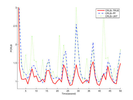
Figure 2: Comparison of the true posterior CRLB with the first type of approximations. The approximated PCRLB corresponds to the method of “exact model and expectation of state estimation”, and were generated by Particle filter (PF) and Unscented Kalman filter (UKF). 100 runs of Monte Carlo simulation.

Figure 3: Comparison of the true posterior CRLB with the second type of approximations. The approximated PCRLB corresponds to the method of “Taylor expanded model and first-two moments of state estimation”, the two estimators: Particle filter (PF) and Unscented Kalman filter (UKF), were employed. $100$ runs of Monte Carlo simulation.

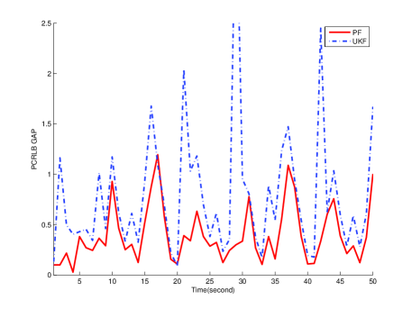
Figure 4: Comparison of two kinds of theoretical gap of posterior CRLB, upper and lower plots corresponds to Unscented Kalman filter (UKF) and Particle filter (PF), respectively. As expected, the gap improve as the accuracy of filtering improves.

For comparison purposes, we implemented two state estimation methods: 1) The unscented Kalman filter (UKF) where it is not necessary to compute Jacobian matrices and the performance is accurate to the third-order term (in the Taylor series expansion) for Gaussian inputs, even for nonlinear systems. For non-Gaussian inputs, approximations are accurate to at least the second-order term [15]. 2) The particle filter (PF), where an initial sample size $N=1000$ is adopted, and $100$ runs of Monte Carlo simulation are performed.

Filtering accuracy by using the same trajectories is shown in Fig.1. Here the root mean square (RMS) error is used as an evaluation criterion. It should be firstly noted that for the PF the initial number of samples is generally chosen by trial-and-error and that its accuracy can be improved by increasing the sample size. Secondly, according to [14], the likelihood $p(y_{k}|x_{k})$ has a bimodal nature when $x_{k}>0$, and this bimodality causes the state too acutely fluctuate and complicates to track using conventional filtering. The RMS error in Fig.1 clearly reflects the effect of the nonlinear dynamic phenomena.

Fig.2 shows the comparison of the true PCRLB and the approach of “exact model and mean of state estimation”, which refers the recursive FIM formulated by (24). We can see from the figure that there exists an explicit error between the true PCRLB and both approximations. The PCRLB corresponding to UKF is overall worse than the PCRLB generated by the PF. As expected, the true PCRLB is a lower bound (always lower than the approximations in all instants).

In Fig.3, the true posterior CRLB is compared with the approach of “Taylor series expanded model and first-two order moments of state estimation”. This approach is performed by substituting Eqn.(16)-(18) into (4) and using first-two order moments of state estimation as parameters. we observe that both estimated PCRLBs are more accurate approximations compared with the true PCRLB. In many instants the PCRLB corresponding to PF is closer to the true PCRLB than the approximation using the UKF. Due to the acute nonlinearity of the system, the PCRLBs appear strongly oscillatory throughout the simulation.

We can directly calculate the difference between the two PCRLB approximations: PCRLB in Fig.2 minus the corresponding one in Fig.3. However, as a theoretical analysis, we employ the formula in (26) and the calculated results are presented in Fig.4. The PCRLB generated by the PF is generally more accurate throughout simulation. When the initial sampling used by PF was increased, the accuracy of its corresponding PCRLB was improved.

VII Conclusion

In this paper, we considered the problem of approximate calculation of CRLB by using Gaussian assumptions and the moments of state estimate instead of using true state. Two kinds of approaches were proposed: One was an exact model using the expectation of state estimate; the other was an approximated model using the expectation and covariance of state estimate. Furthermore, the difference between the two estimated CRLBs was formulated analytically. By using state estimators of PF and UKF, we compared the proposed approximations with true PCRLB. Simulation results demonstrated the significance and validity of our approach.

References

• [1] B. D. O. Anderson and J. B. Moore, Optimal Filtering. Englewood Cliffs, NJ: Prentice-Hall, 1979.
• [2] H. L. van Trees, Detection, Estimation and Modulation Theory. New York: Wiley, 1968.
• [3] T. H. Kerr, Status of CR-like lower bounds for nonlinear filtering, IEEE Trans. Aerosp. Electron. Syst., Vol.25: 590-600, Sept.1989.
• [4] B. Z. Bobrovsky and M.Zakai, A lower bound on the estimation error for Markov processes, IEEE Trans. Automat. Contr., Vol.AC-20: 785-788, Dec.1975.
• [5] Ming Lei, Barend J. van Wyk and Yong Qi, ”Online Estimation of the Approximate Posterior Cramer-Rao Lower Bound for Discrete-time Nonlinear Filtering”, IEEE Trans. on Aerospace and Electronic Systems, to appear.
• [6] J. I. Galdos, A Cramer-Rao bound for multidimensional discrete-time dynamical systems, IEEE Trans. Automat. Contr., Vol.AC-25: 117-119, Feb. 1980.
• [7] P. Tichavsky, C. Muravchik, A. Nehorai, Posterior Cramer-Rao Bounds for Discrete-Time Nonlinear Filtering. IEEE Trans. Signal Processing, Vol.46(5): 1386-1396, May 1998.
• [8] Farina, A., Ristic, B., and Timmoneri, L., Cramer-Rao bound for nonlinear filtering with Pd¡1 and its application to target tracking, IEEE Trans. Signal Process., Vol.50(8):1916-1924. 2002.
• [9] B. Ristic, A. Farina and M. Hernandez, Cramer-Rao lower bound for tracking multiple targets, IEE Proc. Radar Sonar Navig., Vol.151(3):129-134, June 2004.
• [10] RuixinNiu, Peter Willett, and Yaakov Bar-Shalom, Matrix CRLB Scaling Due to Measurements of Uncertain Origin, IEEE Trans. Signal Process., Vol.49(7): 1325-1335, July 2001.
• [11] M. Simandl, J. Kralovec, and P. Tichavsky. Filtering, predictive and smoothing Cramer-Rao bounds for discrete-time nonlinear dynamic systems. Automatica, Vol.37(11):1703-1716, Nov. 2001.
• [12] S.M.Key, Fundamental of Statistical Signal Processing: Estimation Theory, Prentice Hall, Englewood Cliffs, NJ, 1993.
• [13] H.Eves, Elementary Matrix Theory, Dover, New York, 1966.
• [14] Kotecha J.H. and Djuric P.M., Gaussian particle filtering. IEEE Trans. Signal Process., Vol.51(10):2592-2601. Oct. 2003.
• [15] S. J. Julier, J. K. Uhlmann and H. F. Durrant-Whyte. A New Approach for Filtering Nonlinear Systems. The Proceedings of the American Control Conference, Seattle, Washington., pages 1628-1632. 1995.