Magnetic helicity fluxes in interface and flux transport dynamos

Abstract

Context. Dynamos in the Sun and other bodies tend to produce magnetic fields that possess magnetic helicity of opposite sign at large and small scales, respectively. The build-up of magnetic helicity at small scales provides an important saturation mechanism.

Aims. In order to understand the nature of the solar dynamo we need to understand the details of the saturation mechanism in spherical geometry. In particular, we want to understand the effects of magnetic helicity fluxes from turbulence and meridional circulation.

Methods. We consider a model with just radial shear confined to a thin layer (tachocline) at the bottom of the convection zone. The kinetic $\alpha$ owing to helical turbulence is assumed to be localized in a region above the convection zone. The dynamical quenching formalism is used to describe the build-up of mean magnetic helicity in the model, which results in a magnetic $\alpha$ effect that feeds back on the kinetic $\alpha$ effect. In some cases we compare with results obtained using a simple algebraic $\alpha$ quenching formula.

Results. In agreement with earlier findings, the magnetic $\alpha$ effect in the dynamical $\alpha$ quenching formalism has the opposite sign compared with the kinetic $\alpha$ effect and leads to a catastrophic decrease of the saturation field strength with increasing magnetic Reynolds numbers. However, at high latitudes this quenching effect can lead to secondary dynamo waves that propagate poleward due to the opposite sign of $\alpha$. Magnetic helicity fluxes both from turbulent mixing and from meridional circulation alleviate catastrophic quenching.

1 Introduction

The solar dynamo models developed so far and which agree with solar magnetic field observations tend to solve the $\alpha\Omega$ mean field dynamo equations. The turbulent $\alpha$-effect first proposed by Parker (1955) is believed to be generated due to helical turbulence in the convection zone of the Sun. Since $\alpha$ is generated due to quadratic correlations of the small-scale turbulence we need a closure in order to complete the set of mean field equations, e.g., the first order smoothing approximation (FOSA), and express the mean electromotive force in terms of the mean magnetic fields. This turbulent $\alpha$ encounters a critical problem when the energy of the mean field becomes comparable to the equipartition energy of the turbulence in the convection zone and hence it becomes increasingly difficult for the helical turbulence to twist rising blobs of magnetic field. The solar dynamo modellers have traditionally used what is referred to as algebraic alpha quenching to mimic this phenomena. This involves replacing $\alpha$ by $\alpha_{0}/(1+\overline{B}^{2}/B_{\rm eq}^{2})$, an expression used since Jepps (1975), or by $\alpha_{0}/(1+R_{\rm m}\overline{B}^{2}/B_{\rm eq}^{2})$, where $\alpha_{0}$ is the unquenched value and $R_{\rm m}$ is the magnetic Reynolds number, $\overline{B}$ is the mean magnetic field and $B_{\rm eq}$ is the equipartition magnetic field. The latter expression has been discussed since the early work of Vainshtein & Cattaneo (1992). The $R_{\rm m}$ in the denominator comes from the fact that the small-scale fluctuating magnetic field reaches equipartition long before the mean magnetic field does. This has been supported by several numerical experiments to determine the saturation behaviour of $\alpha$ (e.g. Cattaneo & Hughes 1996, Ossendrijver et al. 2002). Given the large magnetic Reynolds numbers of Astronomical objects, such phenomena is referred to as catastrophic quenching.

After the discovery of the layer of strong radial shear (called the tachocline by Spiegel & Zahn 1992) at the bottom of the solar convection zone, Parker (1993) proposed a new class of solar dynamo models called the interface dynamo. In these models the shear is confined to a narrow overshoot layer just beneath the convection zone, also the region of $\alpha$ effect. The dynamo wave propagates in a direction given by the Parker–Yoshimura rule at the interface between the two layers defined by a steep gradient in the turbulent diffusivity. The toroidal field produced due to stretching by the shear is much stronger than the poloidal field and remains confined in the overshoot layer, away from the region where the $\alpha$ effect operates. It may be noted that the interface dynamo model may have serious problems when solar-like rotation with positive latitudinal shear is included (Markiel & Thomas 1999). Similarly, in the Babcock-Leighton class of flux transport models (Choudhuri et al. 1995; Durney 1995) the toroidal and the poloidal fields are produced in two different layers. Unlike in the interface dynamo models, the coupling between the two layers is mediated both by diffusion and the conveyer belt mechanism of the meridional circulation.

It has been proposed that in interface and Babcock-Leighton type dynamos, the $\alpha$ effect is not catastrophically quenched at high $R_{\rm m}$ because the strength of the toroidal field is very weak in the region of finite turbulent $\alpha$ (e.g. Tobias, 1996; Charbonneau, 2005). However, according to our knowledge, not much has been done to study the variation of the amplitude of the saturation magnetic field with the magnetic Reynolds number for these classes of $\alpha\Omega$ dynamos. Zhang et al (2006) made an attempt to reproduce the surface observations of current helicity in the Sun using a 2D mean field dynamo model in spherical coordinates coupled with the dynamical quenching equation. In a separate paper (Chatterjee, Brandenburg & Guerrero, 2010) we have demonstrated that interface dynamo models are also subject to catastrophic quenching.

It has been identified a decade ago that the small-scale magnetic helicity generated due to the dynamo action back reacts on the helical turbulence and quenches the dynamo (Blackman & Field, 2000; Kleeorin et al. 2000). It has now been shown that this mechanism reduces the saturation amplitude of the magnetic field ($B_{sat}$) with increasing magnetic Reynolds number ($R_{\rm m}$). Nevertheless this constraint may be lifted if the system is able to get rid of small scale helicity through several ways like open boundaries, advective, diffusive and shear driven fluxes (Shukurov et al. 2006, Zhang et al. 2006, Sur et al. 2007, Käpylä et al. 2008, Brandenburg et al. 2009, Guerrero et al. 2010). Even though the helicity constraint in direct numerical simulations (DNS) of dynamos with strong shear have been clearly identified, the results can be matched with mean field models having a weaker algebraic quenching than $\alpha^{2}$ dynamos (Brandenburg et al. 2001). It is possible to include this process in mean-field dynamo models through an equation describing the evolution of the small scale current helicity. We shall refer to this equation as the dynamical quenching mechanism.

In this paper we perform a series of calculations with mean field $\alpha\Omega$ models in spherical geometry along with a dynamical equation for the evolution of $\alpha$ for magnetic Reynolds numbers in the range $1\leq R_{\rm m}\leq 2\times 10^{5}$. An important feature of the calculation is that the region of strong narrow shear is separated from the region of helical turbulence. This paper in addition to providing detailed results not mentioned in Chatterjee, Brandenburg & Guerrero (2010), is also aimed at studying somewhat more complicated models including meridional circulation. The role of diffusive helicity fluxes modelled into the dynamical quenching equation by using a Fickian diffusion term is also discussed for various models. It may be mentioned that helicity fluxes across an equator can indeed be modelled by such a diffusion term as shown by Mitra et al. (2010). In §2 we discuss the features of the $\alpha\Omega$ model used, and the formulation of dynamical $\alpha$ quenching. The results are highlighted in §3 and conclusions are drawn in §4.

2 The basic $\alpha\Omega$ Dynamo Model

2.1 Simple two-layer dynamo

We solve the induction equation in a spherical shell assuming axisymmetry. Our dynamo equations consists of the induction equations for the mean poloidal potential $A_{\phi}(r,\theta)$ and the mean toroidal field $B_{\phi}(r,\theta)$. Axisymmetry demands that for all variables $\partial/\partial\phi=0$. Let us first do a qualitative estimate of the turbulent $\alpha$ and the turbulent diffusivity $\eta_{\rm t}$. From mixing length theory we have (cf. Sur et al. 2008),

$$\eta_{\rm t}=\frac{u_{\rm rms}}{3k_{\rm f}},$$

where $u_{\rm rms}$ is the rms velocity of the turbulent eddies, $k_{\rm f}$ is the wavenumber of the energy-carrying eddies, corresponding to the inverse pressure scale height near the base of the convection zone. Since we have made use of the error function profile extensively, let us denote

$$\Theta^{\pm}(r,r_{c},d_{c})=1\pm\textrm{erf}\left(\frac{r-r_{e}}{d_{e}}\right).$$

We have used a smoothed step profile for $\eta_{\rm t}$ given by

$$\eta(r)=\eta_{r}+\eta_{\rm t}\Theta^{+}(r,r_{e},d_{e})$$ (1)

where $r_{e}=0.73R_{\odot}$, and $d_{e}=0.025R_{\odot}$. In this paper we define the magnetic Reynolds number $R_{\rm m}=\eta_{\rm t}/\eta_{r}$. Using FOSA we also have $\alpha_{0}=\tau\epsilon_{\rm f}\omega_{\rm rms}u_{\rm rms}/3$, where $\omega_{\rm rms}$ is the rms vorticity of the turbulence and $\tau\sim(k_{\rm f}u_{\rm rms})^{-1}$ is the eddy correlation time scale. The prefactor $\epsilon_{\rm f}$, usually of order 0.1 or less is used since $({\@vec{u}.\@vec{\omega}})_{\rm rms}<u_{\rm rms}\omega_{\rm rms}$. The case $\epsilon_{\rm f}=1$ means the flow is maximally helical. These approximations give us an estimate of $\alpha_{0}$ in terms of eddy diffusivity $\eta_{\rm t}$ and forcing scale $k_{\rm f}$ as,

$$\alpha_{0}=\epsilon_{\rm f}\frac{\tau k_{\rm f}u_{\rm rms}^{2}}{3}=\epsilon_{\rm f}\eta_{\rm t}k_{\rm f}.$$

We would consider $k_{\rm f}$ rather than $\alpha_{0}$ as a free parameter in the model apart from $\eta_{\rm t}$. Assuming equipartition between magnetic energy and the turbulent energy, we also calculate an equipartition magnetic field $B_{\rm eq}$ as,

$$B_{\rm eq}=(4\pi\rho)^{1/2}u_{\rm rms}=(4\pi\rho)^{1/2}3\eta_{\rm t}k_{\rm f}.$$

For algebraic quenching we consider the following form for kinematic $\alpha_{\rm K}$ given by,

$$\alpha_{\rm K}(r)=\frac{0.5\epsilon_{\rm f}\eta_{\rm t}k_{\rm f}\Theta^{+}(r,r_{a},d_{a})\cos\theta\sin^{q}\theta}{1+g_{\alpha}\overline{B}^{2}/B_{\rm eq}^{2}},$$ (2)

where $g_{\alpha}$ is a non-dimensional coefficient equal to 1 or $R_{\rm m}$ depending on the assumed form of algebraic quenching in the models and $q=0$ unless given. Even though the helical turbulence pervades almost the entire convection zone, we take $r_{a}=0.77R_{\odot}$ and $d_{a}=0.015R_{\odot}$ so that we can have a large separation between the shear and turbulent layer. Consequently we consider a differential rotation profile like that in the high latitude tachocline of the Sun given by,

$$\Omega(r)=-\Omega_{0}\Theta^{+}(r,r_{w},d_{w}),$$ (3)

where $\Omega_{0}=14$nHz, $r_{w}=0.68R_{\odot}$ and $d_{w}=0.015R_{\odot}$. The radial profiles of $\eta_{\rm t}$, $\alpha$ and $\partial\Omega/\partial r$ are plotted as a function of fractional radius $r/R_{\odot}$ in Fig. 1. The region of strong radial shear is separated from the region of helical turbulence and the diffusivity has a strong gradient at a radius lying between the layers of finite strong shear and turbulent $\alpha$. The reason of the same is to decrease the time period $T_{\rm cyl}$ of the oscillatory dynamos to a reasonably small fraction of the diffusion time $t_{\rm diff}$. Our aim is to solve the induction equations coupled with yet another equation for the evolution of $\alpha$-effect, the formulation of which is described in §2.1.

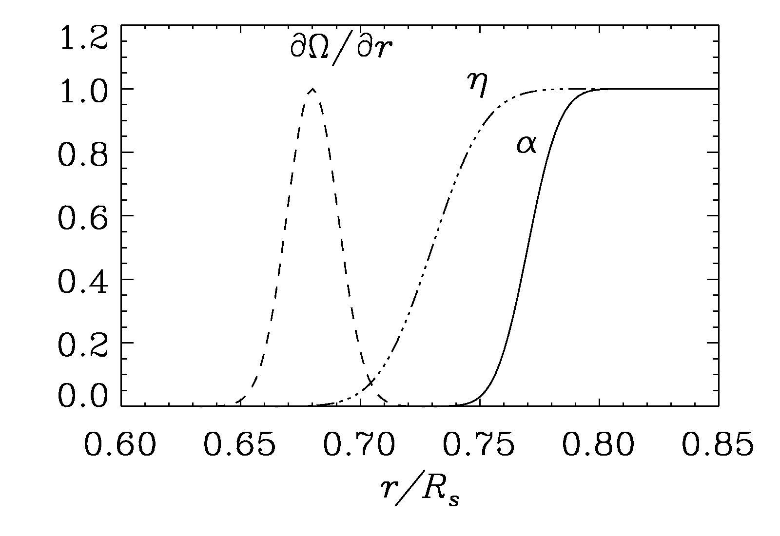
Figure 1: Profiles of radial shear $\partial\Omega/\partial r$ (nHz cm^-1), $\alpha$ (cm s^-1) and $\eta$ ($10^{12}$ cm² s^-1) as a function of fractional solar radius.

2.2 Dynamical $\alpha$ quenching

It was first shown by Pouquet et al. (1976) that the turbulent $\alpha$ effect is modified due to the generation of small-scale helicity in the way given by Eq. (4) below. The second term is sometimes referred to as the magnetic $\alpha$-effect.

$$\alpha=\alpha_{\rm K}+\alpha_{\rm M}=-\frac{\tau}{3}\left(\overline{\@vec{\omega}\cdot\@vec{u}}-\rho^{-1}\overline{\@vec{j\cdot b}}\right),$$ (4)

where $\@vec{\omega}$, $\@vec{u}$, $\@vec{j}$, $\@vec{b}$ denote the fluctuating component of the vorticity, velocity, current and magnetic field in the plasma. It is possible to write an equation for the evolution of the magnetic part of $\alpha$ or $\alpha_{\rm M}$ from the equation for evolution of the small-scale magnetic helicity density $h_{\rm f}=\overline{\@vec{a\cdot b}}$ using the relation,

$$\alpha_{\rm M}=\frac{\eta_{\rm t}k_{\rm f}^{2}}{B_{\rm eq}^{2}}h_{\rm f}.$$ (5)

However the equation for $\overline{\@vec{a\cdot b}}$ will be gauge-dependent and it makes sense only to write an equation for the volume averaged quantity in order to avoid dependence on specific gauge (Blackman & Brandenburg 2002). Our dynamo equations are independent of any gauge since we solve for the magnetic potential component $A_{\phi}$ with an axisymmetric constraint. It is important for us that the equation for $\alpha_{\rm M}$ is also gauge independent. Subramanian & Brandenburg (2006) used the Gauss linking formula for the expression for $h_{\rm f}$ and wrote an equation independent of the gauge for the magnetic helicity density under the assumption that the correlation length for all the fluctuating variables remain small compared to the system size at all times. Using Eq. (5) we write the same equation in terms of $\alpha_{\rm M}$,

$$\frac{\partial\alpha_{\rm M}}{\partial t}=-2\eta_{\rm t}k_{\rm f}^{2}\left(\frac{\overline{\@vec{\mathcal{E}}}\cdot\overline{\@vec{B}}}{B_{\rm eq}^{2}}+\frac{\alpha_{\rm M}}{R_{\rm m}}\right)-\@vec{\nabla}\cdot\overline{\@vec{F}}_{\alpha},$$ (6)

where $\@vec{\mathcal{\overline{E}}}$ and $\overline{\@vec{B}}$ are the mean field EMF and the mean magnetic field. The flux $\overline{\@vec{F}}_{\alpha}$ consists of individual components, e.g., advection due to the mean flow, Vishniac–Cho fluxes (Vishniac & Cho 2001), effects of mean shear, diffusive fluxes, etc. In this paper we have put $\overline{\@vec{F}}_{\alpha}=0$ unless mentioned otherwise.

The decay time in Eq. (6) is $t_{\alpha}=R_{\rm m}/\eta_{\rm t}k_{\rm f}^{2}=4.55\times 10^{-3}R_{\rm m}t_{\rm diff}$. It should be noted that we use $g_{\alpha}=0$ in Eq. (2) whenever we employ the dynamical quenching equation, because dynamical quenching is usually more important.

2.3 Flux transport Babcock-Leighton dynamo

Axisymmetric mean field solar dynamo models including meridional circulation and Babcock-Leighton $\alpha$ effect have been studied extensively by several authors (Dikpati & Charbonneau 1999; Chatterjee et al. 2004; Guerrero & Dal Pino 2008, and references therein). These models have now reached a stage where they are able to reproduce the butterfly diagram and the correct phase between the polar fields and the toroidal fields. In this section we will use a Babcock-Leighton (BL) $\alpha$ along with an analytical meridional circulation (MC) which is poleward at the surface with a maximum amplitude of $u_{0}=20$ m s^-1 and the expression for which is given by van Ballegooijen & Choudhuri (1988). For completeness we provide the expressions for the radial and the latitudinal components of the meridional flow, $\@vec{u}_{p}$ here.

$$u_{r}=u_{0}\left(\frac{R_{\odot}}{r}\right)^{2}\zeta\left(-\frac{2}{3}+\frac{c_{s1}}{2}{\zeta}^{1/2}-\frac{4c_{s2}}{9}{\zeta}^{3/4}\right)(2\cos^{2}\!\theta-\sin^{2}\!\theta),$$ (7)

$$u_{\theta}=u_{0}\left(\frac{R_{\odot}}{r}\right)^{3}(-1+c_{s1}\zeta^{1/2}-c_{s2}\zeta^{3/4})\sin\theta\cos\theta,$$ (8)

where $\zeta=R_{\odot}/r-1$, $r_{b}=0.71R_{\odot}$, $\zeta_{b}=R_{\odot}/r_{b}-1$, $c_{s1}=4\zeta_{b}^{-1/2}$ and $c_{s2}=3\zeta_{b}^{-3/4}$. It should be mentioned that, unlike in flux transport dynamo models, the meridional circulation does not reverse the direction of propagation of the dynamo wave in interface dynamo models as long as the meridional circulation is confined within the convection zone (Petrovay & Kerekes 2004). We solve this model along with the equation for dynamical $\alpha$ quenching described in Sect. 2.1. The fluxes in Eq. (6) are now given by,

$$\overline{\@vec{F}}_{\alpha}=\alpha_{\rm M}{\@vec{u}}_{\rm p}-\@vec{\nabla}\cdot(\kappa\@vec{\nabla}\alpha_{\rm M}),$$ (9)

where $\kappa$ is the diffusion coefficient for $\alpha_{\rm M}$ taken to be $\kappa_{0}\eta(r)$. It may be remembered that the $\alpha_{\rm K}$ is now not due to the helical turbulence in the bulk of the convection zone, but due to a phenomenological BL $\alpha$ where the poloidal field is produced from the toroidal field due to decay of tilted bipolar active regions. The analytical expression for $\alpha_{\rm K}$ is given by

$$\alpha_{\rm K}=\frac{1}{4}\alpha_{\rm BL}\Theta^{+}(r,0.95R_{\odot},d)\;\Theta^{-}(r,R_{\odot},d)\cos\theta\sin^{2}\theta$$ (10)

with $d=0.015R_{\odot}$. The BL $\alpha$ is assumed to be concentrated only in the upper 0.05% of the convection zone. The turbulent diffusivity has the same profile as in Eq. (1) but with $\eta_{\rm t}=2\times 10^{11}$ cm s^-1 and $r_{e}=0.7R_{\odot}$. The shear is still radial and given by Eq. (3) with $r_{w}=0.7R_{\odot}$.

Our computational domain is defined to be the region confined by $0\leq\theta\leq\pi$ and $0.55R_{\odot}\leq r\leq R_{\odot}$. Unless otherwise stated, the boundary conditions for $A_{\phi}$ are given by a potential field condition at the surface (Dikpati & Choudhuri 1994) and $A_{\phi}=0$ at the poles. We have also performed some calculations with the vertical field condition at the top boundary, which means that $B_{\theta}=B_{\phi}=0$. At the bottom we use the perfect conductor boundary condition of Jouve et al. (2008) with $A_{\phi}=\partial(rB_{\phi})/\partial r=0$. However a more realistic perfect conductor boundary condition in our opinion would be $\partial(rB_{\theta})/\partial r=\partial(rB_{\phi})/\partial r=0$. Also $B_{\phi}=0$ on all other boundaries. The equation for $\alpha_{\rm M}$ is an initial value problem for $F_{\alpha}=0$. For finite fluxes we have also set $\alpha_{\rm M}=0$ at all boundaries. We have checked that the results are not very sensitive to the different boundary conditions given above mainly because the boundaries are far removed from the dynamo region.

3 Results

3.1 Magnetic field properties without helicity fluxes

In order to study the $R_{\rm m}$ dependence of the saturation magnetic field in the two layered dynamo with diffusive coupling we keep all the dynamo parameters the same for all the runs and change $\eta_{r}$ from $2\times 10^{5}$ cm² s^-1 to $2\times 10^{10}$ cm² s^-1 while keeping $\eta_{\rm t}$ fixed at $4\times 10^{10}$ cm² s^-1. It may also be noted that the time period of the dynamo models ($T_{\rm cyl}$) is fairly independent of the magnetic Reynolds number. We show the magnetic energies as a function of time for the nonlinear system with $\alpha_{0}=0.08\eta_{\rm t}k_{\rm f}$ for a range of magnetic Reynolds numbers in Fig. 2. The strong $R_{\rm m}$ dependence which is reminiscent of catastrophic quenching in all astrophysical dynamos can be easily discerned from Fig. 2. It is interesting that the saturation energy of the $R_{\rm m}=1$ model is lower than that of the $R_{\rm m}=20$ case. The dynamo model may be highly dissipative at very low magnetic Reynolds numbers.

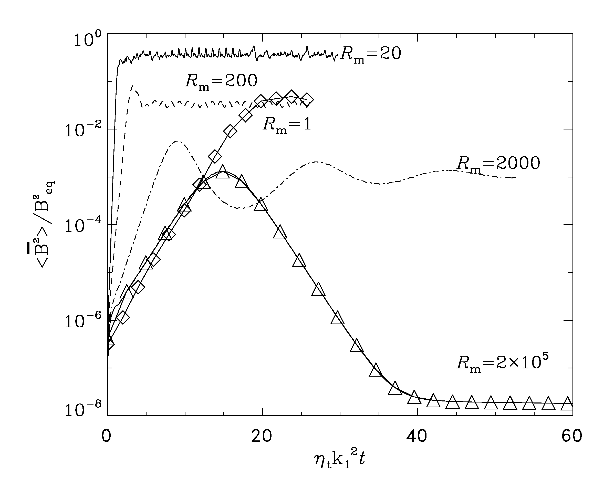
Figure 2: Magnetic energy in the domain scaled with the equipartition energy for $R_{\rm m}=1$ (diamond+line), $R_{\rm m}=20$ (solid), $R_{\rm m}=200$ (dashed), $R_{\rm m}=2\times 10^{3}$(dashed-dotted), $R_{\rm m}=2\times 10^{5}$ (triangles+line) for $\alpha_{0}=0.08\eta_{\rm t}k_{\rm f}$ for the $R_{\rm m}$ indicated in the figure.

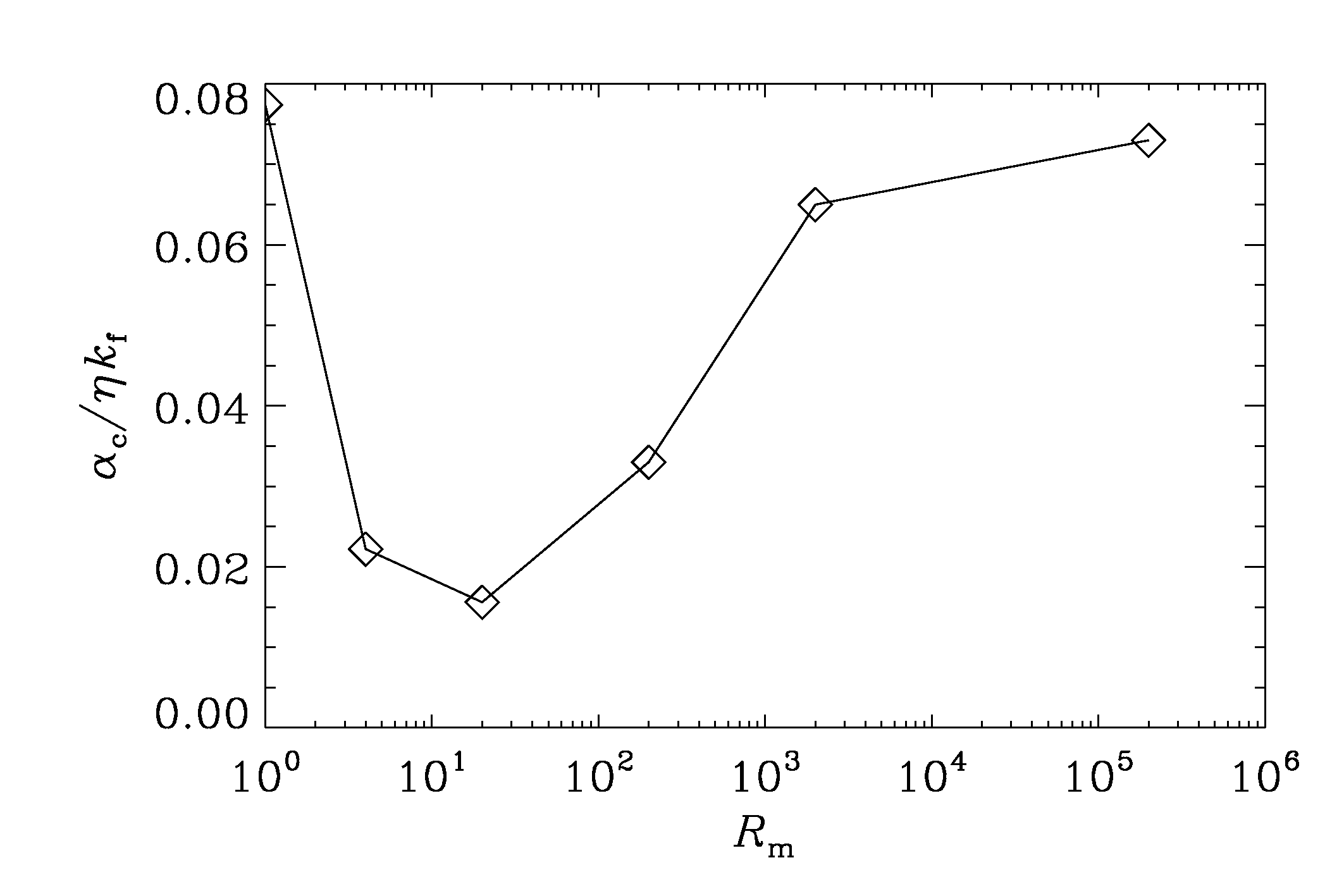
Figure 3: Critical $\alpha$ in terms of a fraction of $\eta_{\rm t}k_{\rm f}$ as a function of magnetic Reynolds number $R_{\rm m}$ for the interface dynamo model of Fig. 1.

The slopes of the volume averaged energy are also very different in the kinematic phase, which means that the critical dynamo numbers also depend on $R_{\rm m}$. To be able to correctly compare the dynamo models for different $R_{\rm m}$, it is first important to calculate the critical value of $\alpha_{0}$, denoted by $\alpha_{c}$ for each model. Such a plot is shown in Fig. 3. From this figure we can conclude that this dynamo model is most efficient near $R_{\rm m}=20$. A similar variation of $\alpha_{c}$ with the ratio $\eta_{\rm t}/\eta_{r}$ was obtained analytically for interface dynamos by MacGregor & Charbonneau (1997; see their Fig. 5A). We now set $\alpha_{0}=2\alpha_{c}$, corresponding to the $R_{\rm m}$ of each model, and repeat our calculations. We shall now use this value of $\alpha$ for the rest of the paper. The saturation energy decreases monotonically as a function of magnetic Reynolds number as shown in Fig. 5. For $R_{\rm m}=2\times 10^{5}$, the code has to be run for 500 $t_{\rm diff}$ before the dynamo field starts becoming ’strong’ again for the case with $\alpha_{0}=2\alpha_{c}$. Due to long computational times involved in this exercise we have not continued the calculation beyond 60 $t_{\rm diff}$. Hence, the determination of saturation magnetic energy may be inaccurate for $R_{\rm m}=2\times 10^{5}$. Compare this with the case of a simple algebraic quenching of the form given in Eq. (2) with $g_{\alpha}=1$. The slopes in the kinematic phase are now almost similar for all $R_{\rm m}$ within the error in the numerical determination of the critical $\alpha_{c}$. For $g_{\alpha}=R_{\rm m}$, the algebraically and dynamically quenched $\alpha$ effects seem to give similar dependences on $R_{\rm m}$. It may occur that the two source regions may not be spatially separated, so we repeat our calculations with the $\alpha$ region at $r_{a}=0.87R_{\odot}$ instead of $0.77R_{\odot}$ and obtain the same slope in the relation of the volume averaged magnetic energy on $R_{\rm m}$ as in Fig. 5. We also verify from the profiles of field components at two different latitudes, as shown in Fig. 6, that the region of strong toroidal field $B_{\phi}$ is different from the layer where poloidal fields are produced by the $\alpha$ effect.

Figure 4: Magnetic energy in the domain scaled with the equipartition energy for $R_{\rm m}=1$ (diamond+line), $R_{\rm m}=20$ (solid), $R_{\rm m}=200$ (dashed), $R_{\rm m}=2\times 10^{3}$ and $R_{\rm m}=2\times 10^{5}$ (triangles) with algebraic quenching for $g_{\alpha}=1$

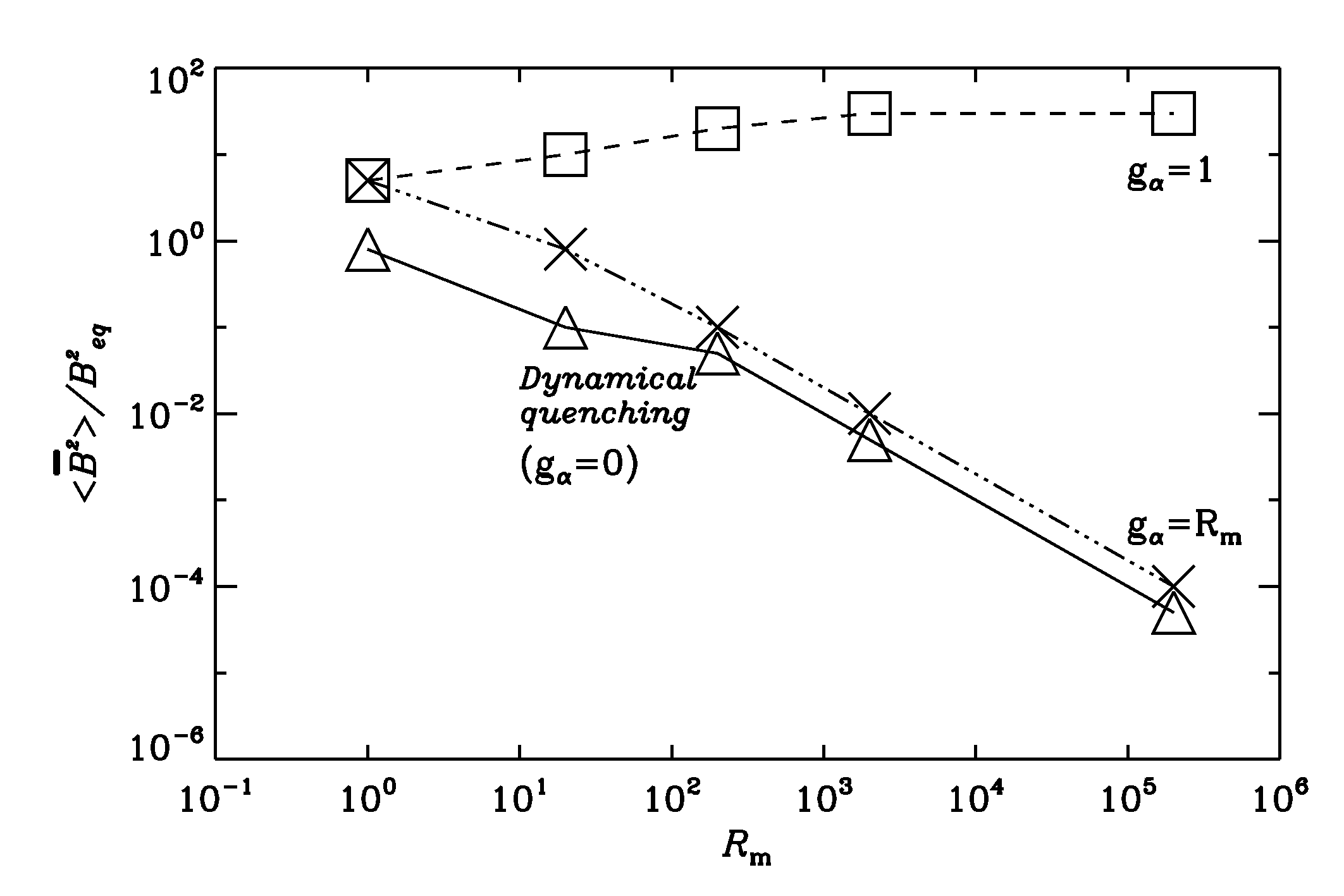
Figure 5: Volume averaged magnetic energy scaled with the equipartition energy in the saturation phase as a function of $R_{\rm m}$ for dynamical $\alpha$ quenching (triangles +solid) and algebraic quenching with $g_{\alpha}=1$ (squares + dashed) and with $g_{\alpha}=R_{\rm m}$ (cross + dashed-dotted).

For the solutions with dynamical $\alpha$ effect, it may be concluded from the butterfly diagrams of Fig. 7 that the small-scale current helicity $\alpha_{\rm M}$ is predominantly negative (positive) in the Northern (Southern) hemisphere. The nature of the saturation curves of the magnetic energy is strongly governed by the ratio of $t_{\alpha}$ and $T_{\rm cyl}$. For $R_{\rm m}=20$, $t_{\alpha}\ll T_{\rm cyl}=0.85t_{\rm diff}$ and so there are strong oscillations in the butterfly diagram for $\alpha_{\rm M}$, as shown in Fig. 7a, whereas for $R_{\rm m}=200$, $t_{\alpha}\sim T_{\rm cyl}$ the amplitude of oscillations is weak because the $\alpha_{\rm M}$ decays at the same rate at which it is produced due to the effect of the oscillatory source term $\@vec{\mathcal{E}}\cdot\overline{\@vec{B}}$; see Fig. 7b. Similarly for $R_{\rm m}=2\times 10^{3}$, the decay time $t_{\alpha}\gg T_{\rm cyl}$ and so the system of equations is overdamped as can be seen from the saturation curve (dashed dotted line) in Fig. 2b where there are amplitude modulations of the magnetic field before it settles to a final saturation value. When the code is run longer, we start seeing changes in the parity after $t>40t_{\rm diff}$. However the magnetic energy and the dynamo period $T_{\rm cyl}$ remain fairly constant even while the system fluctuates between symmetric and anti-symmetric parity at an irregular time interval (see Fig. 8). This parity oscillation is absent in the corresponding models with algebraic quenching.

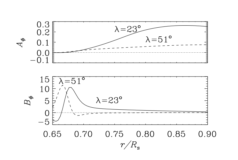
Figure 6: Radial profiles of $A_{\phi}$ and $B_{\phi}$ at two different latitudes ($\lambda$) in the saturated phase for $R_{\rm m}=2\times 10^{3}$.

3.2 Secondary dynamo waves

An interesting result emerges when we repeat our calculations with $\alpha_{0}=4\alpha_{c}$ instead of $2\alpha_{c}$ for $R_{\rm m}=20$. The negative $\alpha_{\rm M}$ generated in the convectively unstable layer penetrates below 0.73$R_{\odot}$ where $\alpha_{\rm K}=0$ and drives a secondary dynamo wave whose direction of propagation is poleward as compared to the primary dynamo wave propagating equatorward. This can be seen in the butterfly diagram of $B_{\phi}$ at 0.72$R_{\odot}$ in Fig. 9a. Signature of the secondary dynamo can also be seen in the butterfly diagram at 0.8$R_{\odot}$. Even though the secondary dynamo wave is energetically powered by the kinematic part of the helical convection but the direction of propagation is governed by the sign of $\alpha_{\rm K}+\alpha_{\rm M}$. This may be compared with an $\alpha\Omega$ dynamo driven by a supercritical helicity flux (Vishniac & Cho 2001). This mechanism however requires finite initial magnetic field. It may be recalled that we have done calculations with an initial field $\sim 10^{-6}B_{\rm eq}$. The difference compared to the case above is that the mean field dynamo is not driven by supercritical Vishniac & Cho fluxes, but it is governed by a local generation of small-scale magnetic helicity. We return to the issue of secondary dynamo waves driven by diffusive magnetic helicity fluxes in Sect. 3.3.

We also have not observed any evidence of chaotic behaviour in the range of magnetic Reynolds number $20\leq R_{\rm m}\leq 2\times 10^{5}$ for supercritical $\alpha\leq 4\alpha_{c}$ in agreement with Covas et al. (1998). However, if the $\alpha$ effect is highly supercritical, the dynamical quenching formula for $\alpha_{\rm M}$ is insufficient for dynamo saturation, and additional algebraic quenching terms must enter (Kleeorin & Rogachevskii 1999).

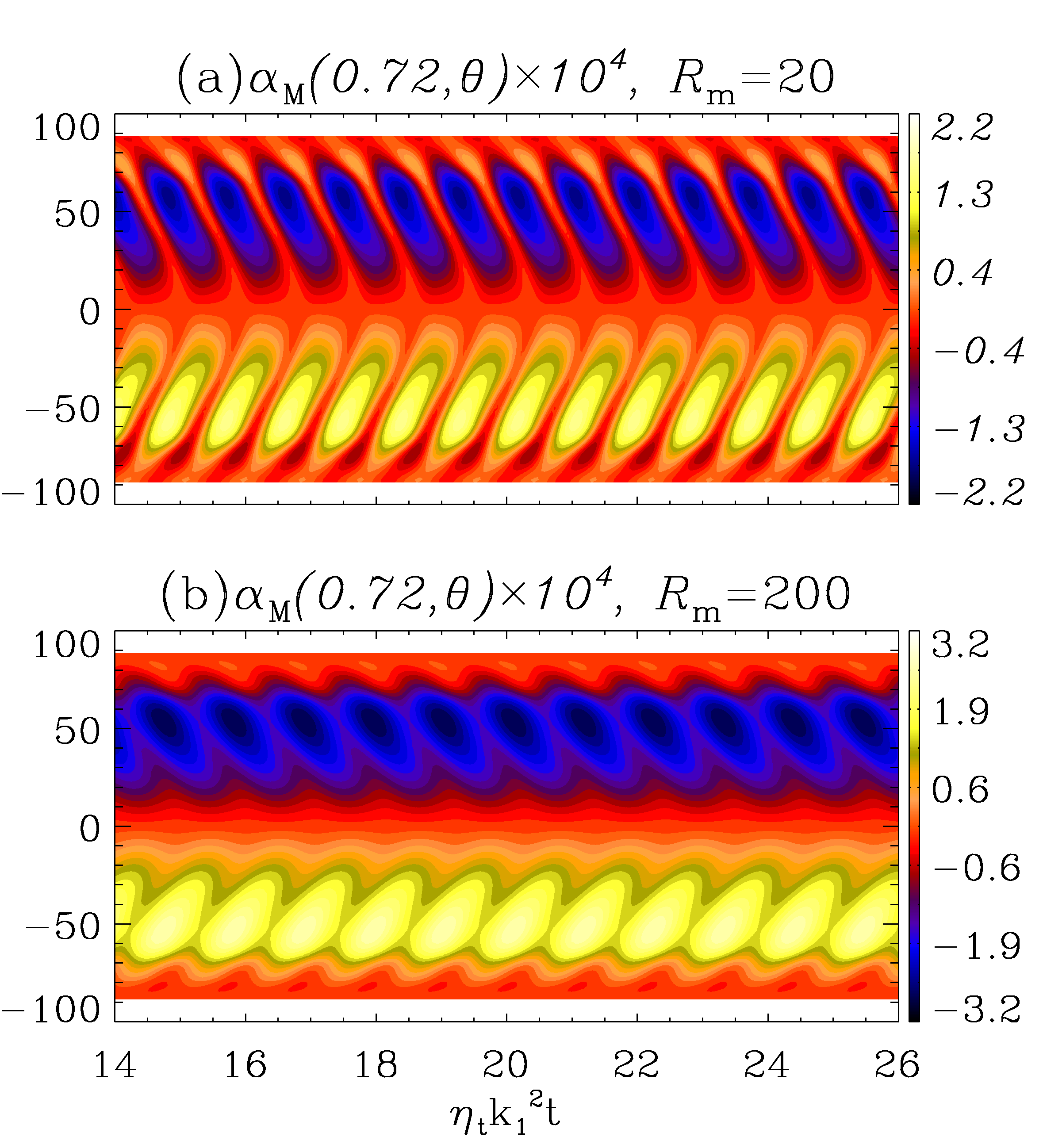
Figure 7: $\alpha_{\rm m}(0.72R_{\odot},\theta)$ as a function of diffusion time $\eta_{\rm t}k_{1}^{2}t$ for (a) $R_{\rm m}=20$ and (b) $R_{\rm m}=200$.

3.3 Diffusive magnetic helicity fluxes

Recently, Brandenburg et al. (2009) showed that catastrophic quenching in one-dimensional $\alpha^{2}$ dynamos can be alleviated by introducing a Fickian diffusive flux in Eq. (6) given by

$$\overline{\@vec{F}}_{\alpha}=-\kappa\@vec{\nabla}\alpha_{\rm M}.$$ (11)

There was an attempt to calculate the diffusion coefficient $\kappa$ from direct numerical simulations and it was found to be $\sim 0.3\eta_{\rm t}$ for $R_{\rm m}\sim 20$ (Mitra et al. 2010). For $\kappa=0$, the saturation curves in Fig. 2b show that the $B_{\rm sat}$ goes through very low values for $R_{\rm m}\sim 2\times 10^{5}$ and it takes very long to relax to a steady amplitude. Next we introduce a diffusive flux with $\kappa(r)=\kappa_{0}\eta(r)$ in Fig. 10 and obtain $B_{\rm sat}\sim 0.1B_{\rm eq}$ and underdamped behaviour. However looking carefully at the corresponding butterfly diagrams (Fig. 11a,b,c,d) we find a poleward propagating mode due to radial diffusion of the $\alpha_{\rm M}$ into the stable layers which otherwise was not possible for a very high $\eta_{\rm t}/\eta_{r}$ ratio. Figures 11e,f show meridional snapshots of $\textrm{sign}(B_{\phi})(|B_{\phi}|/B_{\rm eq})^{1/2}$ and $\alpha_{\rm M}$ in order to get a clearer idea of the distribution of magnetic fields. The poleward propagating mode is now driven by supercritical diffusive helicity fluxes, as opposed to supercritical Vishniac & Cho fluxes (see Brandenburg & Subramanian 2005 for examples of such behaviour). There exists a $\kappa_{c}\sim 10^{-5}$ for $R_{\rm m}=2\times 10^{5}$ such that the secondary dynamo fails to operate if $\kappa_{0}<\kappa_{c}$ and the volume averaged magnetic energy decays eventually. It should be noted that this threshold for $\kappa$ is highly dependent on $R_{\rm m}$. For instance $R_{\rm m}=2\times 10^{3}$ and $\kappa_{0}=10^{-5}$ produces a dynamo with finite saturation magnetic field and dynamo wave propagation governed by $\alpha_{M}$ where as for $\kappa=10^{-4}\eta$, the dynamo shows a runaway growth. An interesting behaviour can be discerned from the butterfly diagram of the toroidal field for $R_{\rm m}=2\times 10^{3}$ and $\kappa_{0}=10^{-5}$ (Fig.10b,c). It appears that the behaviour of the dynamo is governed by competition between the poleward propagating mode and the equatorward propagating mode. The volume averaged energy (stars+line in Fig.10a) shows corresponding oscillations long after saturation at an period $\sim 5$ times the period of the equatorward propagating mode. It may be recalled that it is well established from direct numerical simulations of $\alpha^{2}$ dynamos that a large-scale magnetic field is easily excited on the scale of the system i.e., $k_{1}^{-1}$ for a large $k_{\rm f}/k_{1}$ ratio (Archontis, Dorch, Nordlund, 2003). The length scale of the magnetic field in Figs.10b,c and Figs. 11a,c,e is comparable to $k_{\rm f}^{-1}$, which suggests that the degree of scale-separation may have become insufficient to write the electromotive force as a simple multiplication, as is done in the expression $\overline{\@vec{\mathcal{E}}}=\alpha\overline{\@vec{B}}-\eta\overline{\@vec{J}}$, and that it may have become necessary to write it as a convolution, which corresponds essentially to a low-pass filter (see, e.g., Brandenburg et al. 2008). However, we have not pursued this aspect any further.

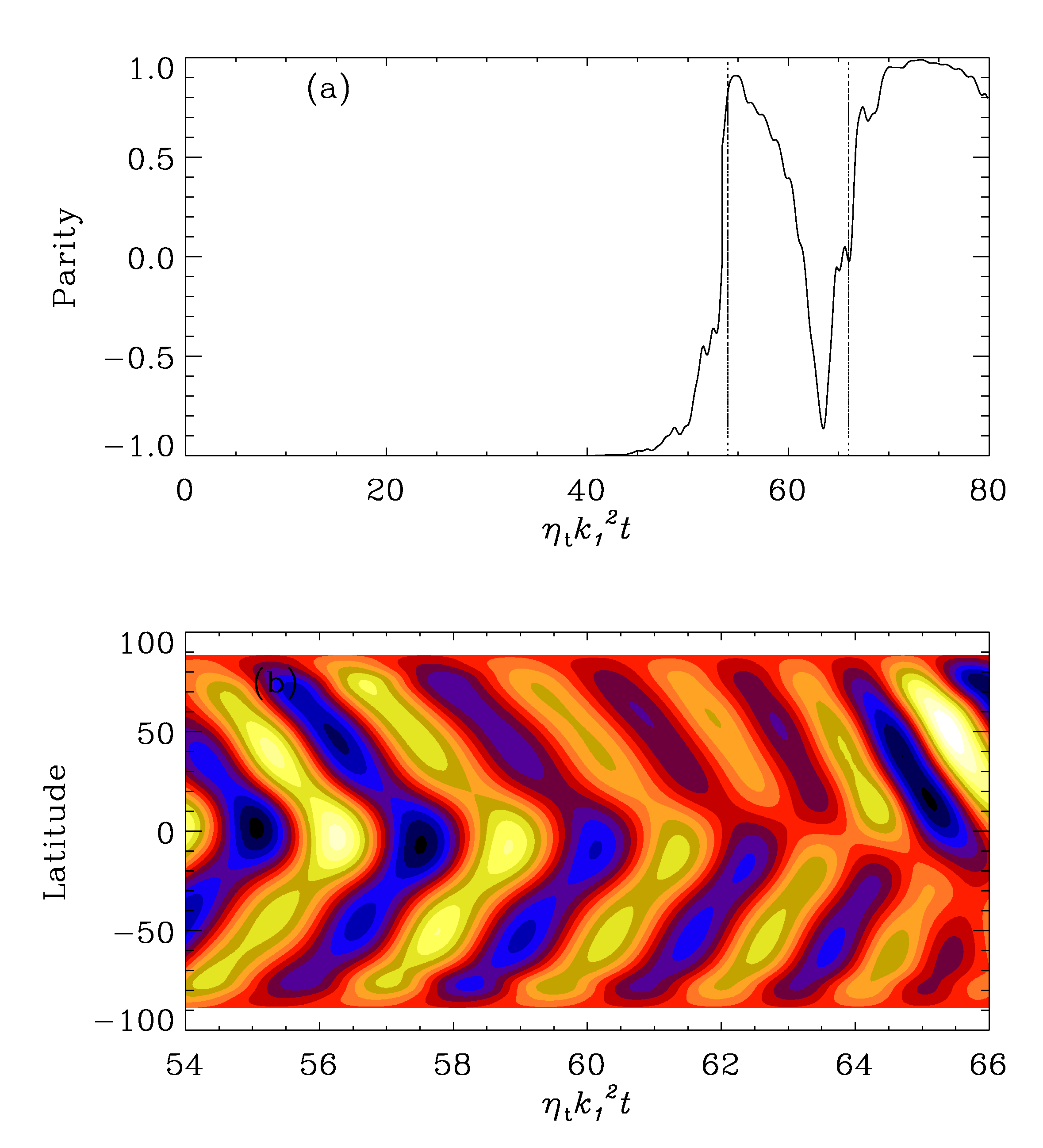
Figure 8: (a) Evolution of parity (purely dipolar $=-1$ and purely quadrupolar $=+1$) for $R_{\rm m}=2\times 10^{3}$. (b) A small part in the butterfly diagram indicated by dotted lines in (a) where parity is changing from quadrupolar to dipolar.

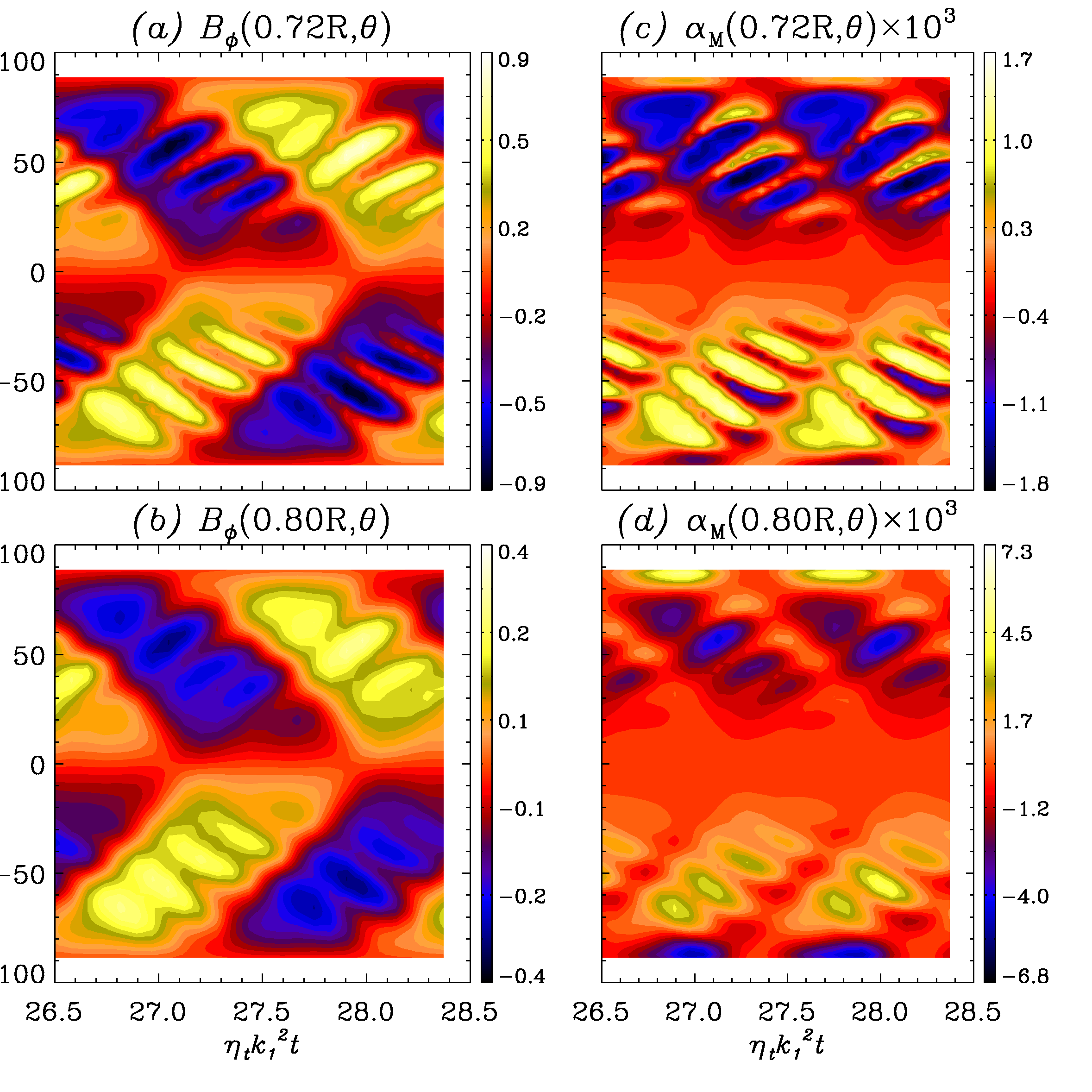
Figure 9: Butterfly diagrams of the toroidal field (a) and (c) and $\alpha_{\rm m}$ (b) and (d) with $\alpha=4\alpha_{c}$ for $R_{\rm m}=20$.

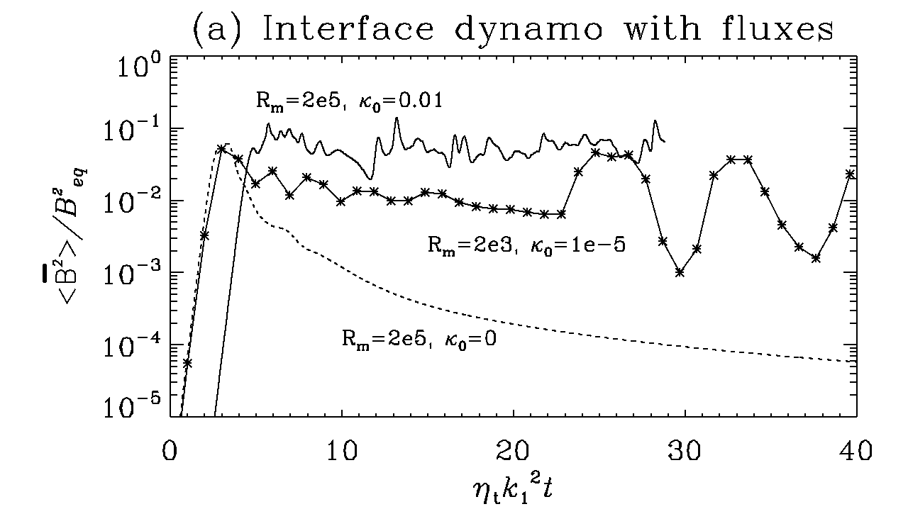
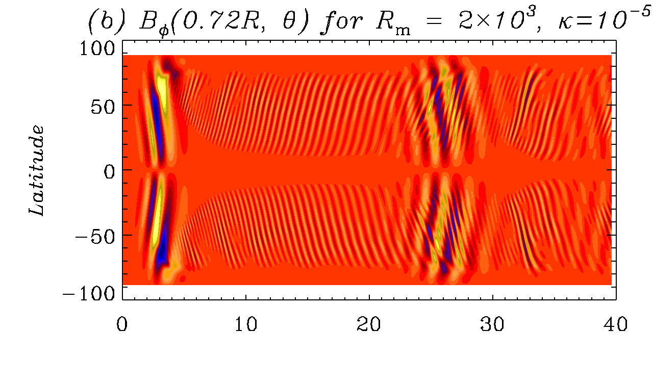
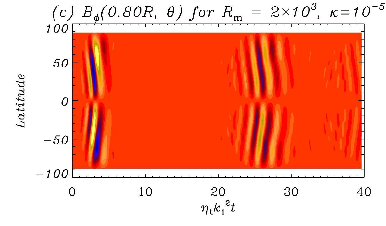
Figure 10: (a) Magnetic energy in the domain scaled with the equipartition energy for $R_{\rm m}=2\times 10^{3}$ indicated in the figure for the case of two layered dynamo of Sect. 3.1 with dynamical $\alpha$ quenching with a diffusive flux with $\kappa_{0}=10^{-5}$ (star+solid). The same for $R_{\rm m}=2\times 10^{5}$ and $\kappa_{0}=10^{-2}$ (solid). The saturation curve for zero fluxes have been shown by the dashed line. (b) and (c) show butterfly diagrams for the toroidal field at the depths indicated for $R_{\rm m}=2\times 10^{3}$ and $\kappa_{0}=10^{-5}$.

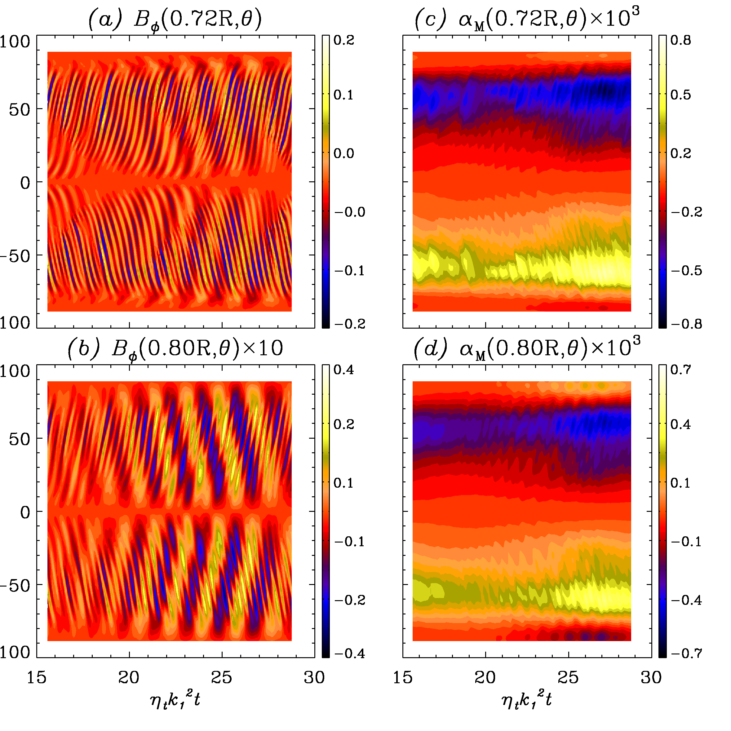
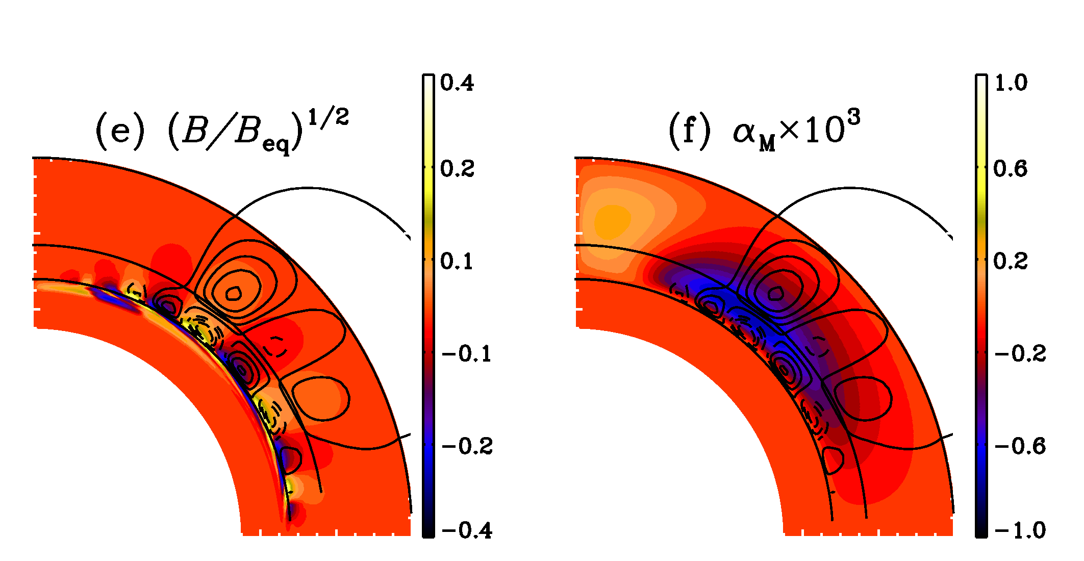
Figure 11: Butterfly diagrams of the toroidal field (a) and (c) and $\alpha_{\rm m}$ (b) and (d) with $\alpha=2\alpha_{c}$ for $R_{\rm m}=2\times 10^{5}$ with a $\kappa_{0}=0.01\eta_{\rm t}$. Meridional snapshots of (e) $(B/B_{\rm eq})^{1/2}$ and (f) $\alpha_{\rm m}\times 10^{3}$ for the same case.

3.4 Flux transport Babcock-Leighton Dynamo

Like in §3.1 we find the critical $\alpha_{\rm BL}$ required to have a self excited dynamo. In this case $\alpha_{c}=5.1$ m s^-1 for $R_{\rm m}=2\times 10^{3}$. We pursue the rest of the calculations with $\alpha_{\rm BL}=6.0$ m s^-1 in order to avoid producing very large $\alpha_{\rm M}$ leading to secondary dynamos discussed in §3.1. We should emphasize that Eq. (4) represents a first order correction to the $\alpha$ and should be treated with caution during its use in supercritical regimes.

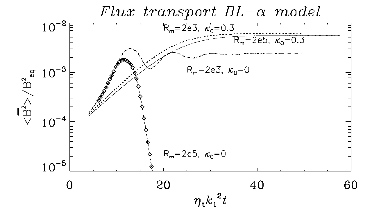
Figure 12: $B^{2}/B_{\rm eq}^{2}$ for the flux transport dynamo model of §3.2 for $R_{\rm m}=2\times 10^{3}$ with $\kappa_{0}=0.3$ (dashed); $R_{\rm m}=2\times 10^{5}$ with $\kappa_{0}=0.3$ (solid); $R_{\rm m}=2\times 10^{3}$ with $\kappa=0$ (dashed-dotted); $R_{\rm m}=2\times 10^{5}$ with $\kappa_{0}=0$ (diamond+dashed).

At first we artificially turn off the advective flux due to meridional circulation as well as the diffusive flux only in Eq. (6), while having them in the induction equations for $B_{\phi}$ and $A_{\phi}$. The saturation curve for $R_{\rm m}=2\times 10^{3}$ is now over-damped whereas the dynamo fails to generate a finite $B_{sat}$ for $R_{\rm m}=2\times 10^{5}$ even though it initially has the same growth rate. On increasing $\alpha_{BL}=10$ ms^-1 from 6 ms^-1 the saturation curve for $R_{\rm m}=2\times 10^{5}$ also displays overdamped behaviour. This indicates that the total $\alpha$ in the domain was simply becoming sub-critical and the dynamo was not able to sustain itself through the saturation phase. We show the distribution of magnetic helicity in the meridional plane for in Fig. 13a, b. Note that $\alpha_{M}$ inside the domain is larger for $R_{\rm m}=2\times 10^{5}$ compared to $R_{\rm m}=2\times 10^{3}$ for the same value of $\alpha_{\rm BL}$.

Inclusion of meridional circulation in Eq. (6) means that we also require a diffusive flux in Eq. (6) to keep the system numerically stable. A diffusive flux in this equation is known to alleviate catastrophic quenching in $\alpha^{2}$ (Brandenburg et al. 2009) as well as $\alpha\Omega$ dynamos (Guerrero, Chatterjee & Brandenburg 2010). It is clear from Fig. 12 that the overdamped behaviour after the end of the kinematic phase is suppressed due to a diffusive flux of $\alpha_{\rm M}$ which essentially reduces the effective decay time for $\alpha_{\rm M}$ to much less than $R_{\rm m}/\eta_{\rm t}k_{\rm f}^{2}$. It may be noted that the dependence of the saturation value of the magnetic energy on $R_{\rm m}$ is now much weaker than the corresponding variation without fluxes. In presence of diffusive and advective fluxes due to meridional circulation in Eq. (6) the small-scale helicity is distributed through out the convection zone as shown in Fig. 14a, b. It is instructive to compare the weaker magnitudes of $\alpha_{\rm M}$ with Fig. 13.

The diffusive fluxes are therefore crucial for operation of a successful mean field $\alpha\Omega$ dynamo. However an interesting observation is the distribution of $\alpha_{M}$ in the concentrated region at the lower part of the convection zone (see Fig. 13) in contrast to Fig. 14. Even though $\alpha_{BL}$ is a surface phenomena, considerable magnetic helicity is generated when the meridional circulation sinks the poloidal field lines at high latitudes and brings them near the tachocline where toroidal fields are generated.

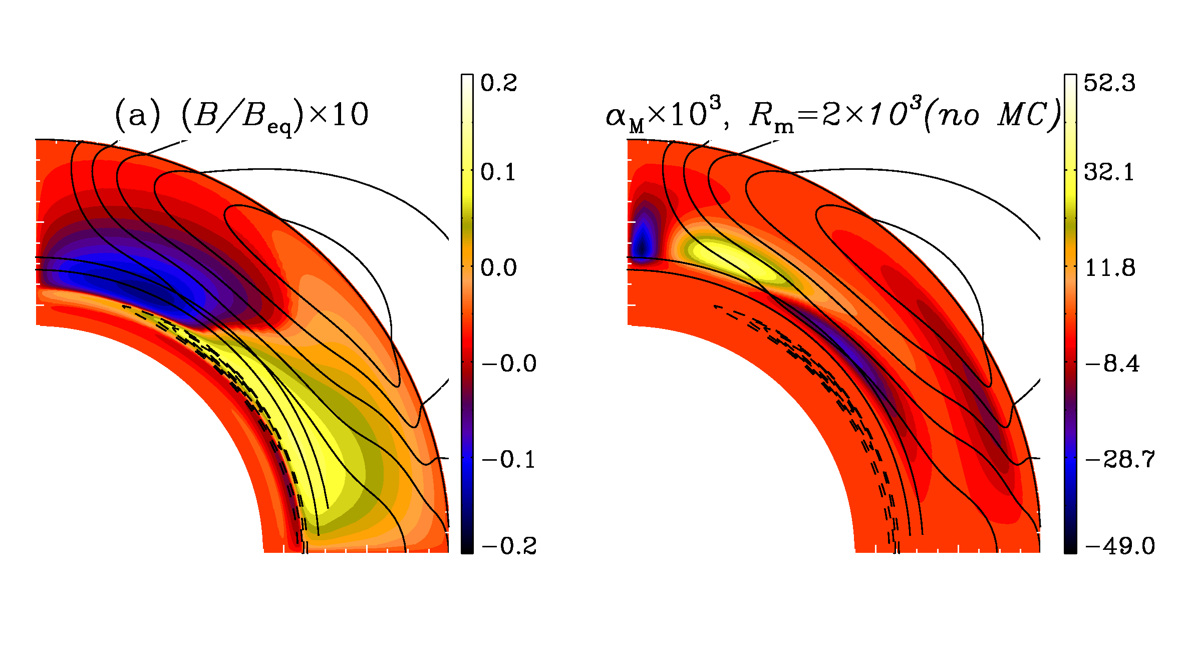
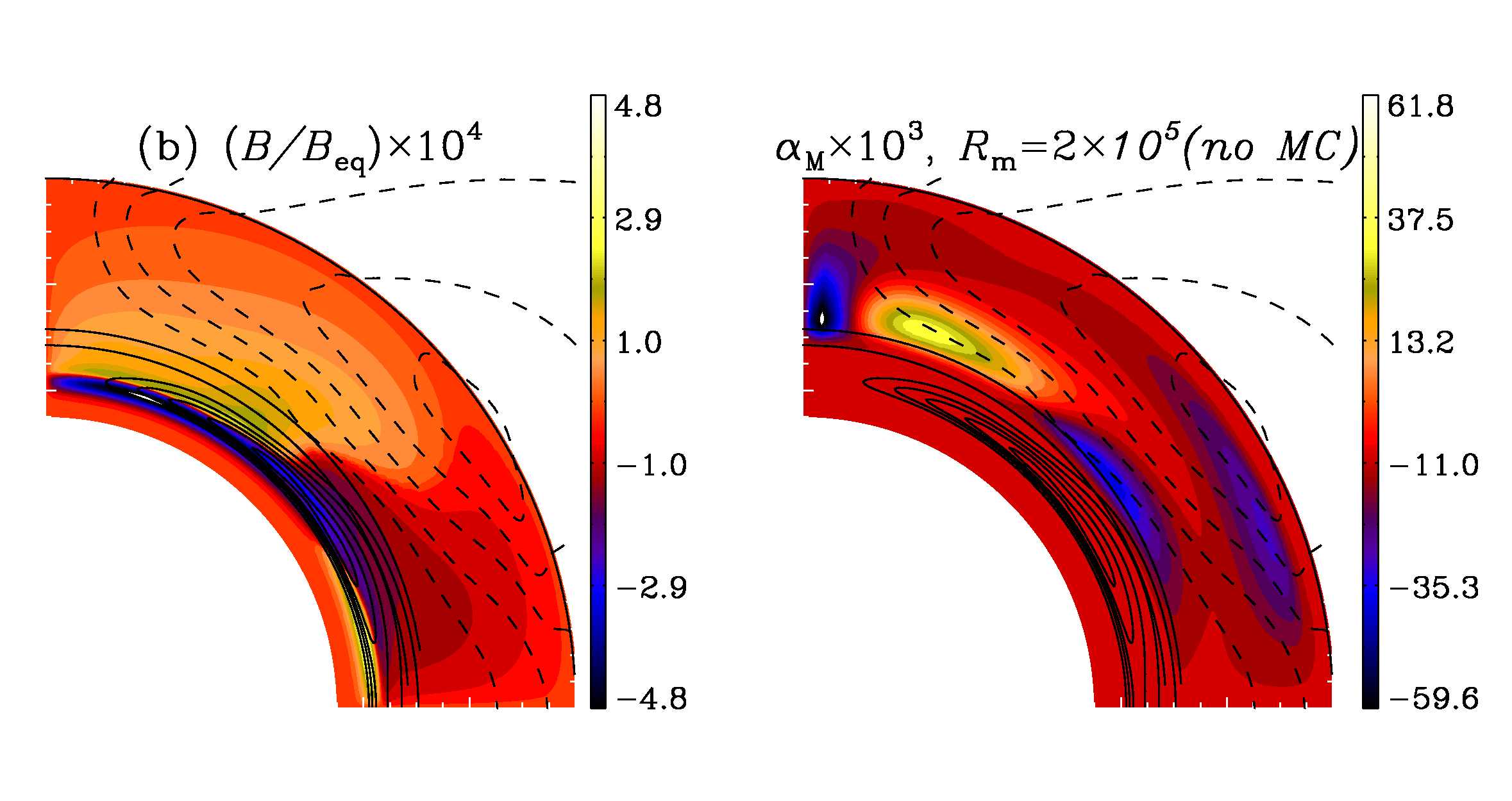
Figure 13: Meridional cross-sections showing the distribution of toroidal field and $\alpha_{M}$ for a Babcock-Leighton dynamo without MC and diffusive helicity fluxes in Eq. 6 for (a) $R_{\rm m}=2\times 10^{3}$ and (b) $R_{\rm m}=2\times 10^{5}$. The streamlines of the positive and negative poloidal field are shown by solid and dashed lines respectively. Note that the magnetic field has decayed to very small values for $R_{\rm m}=2\times 10^{5}$.

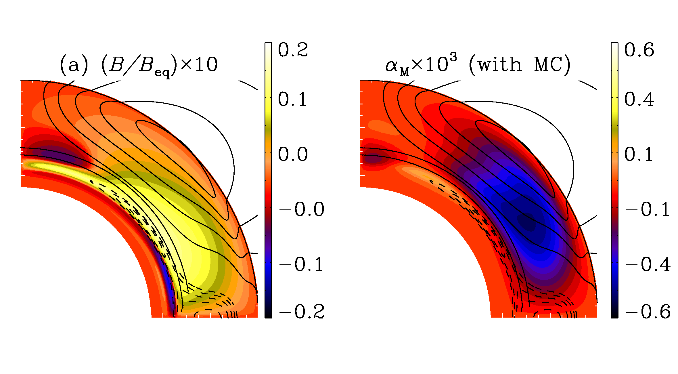
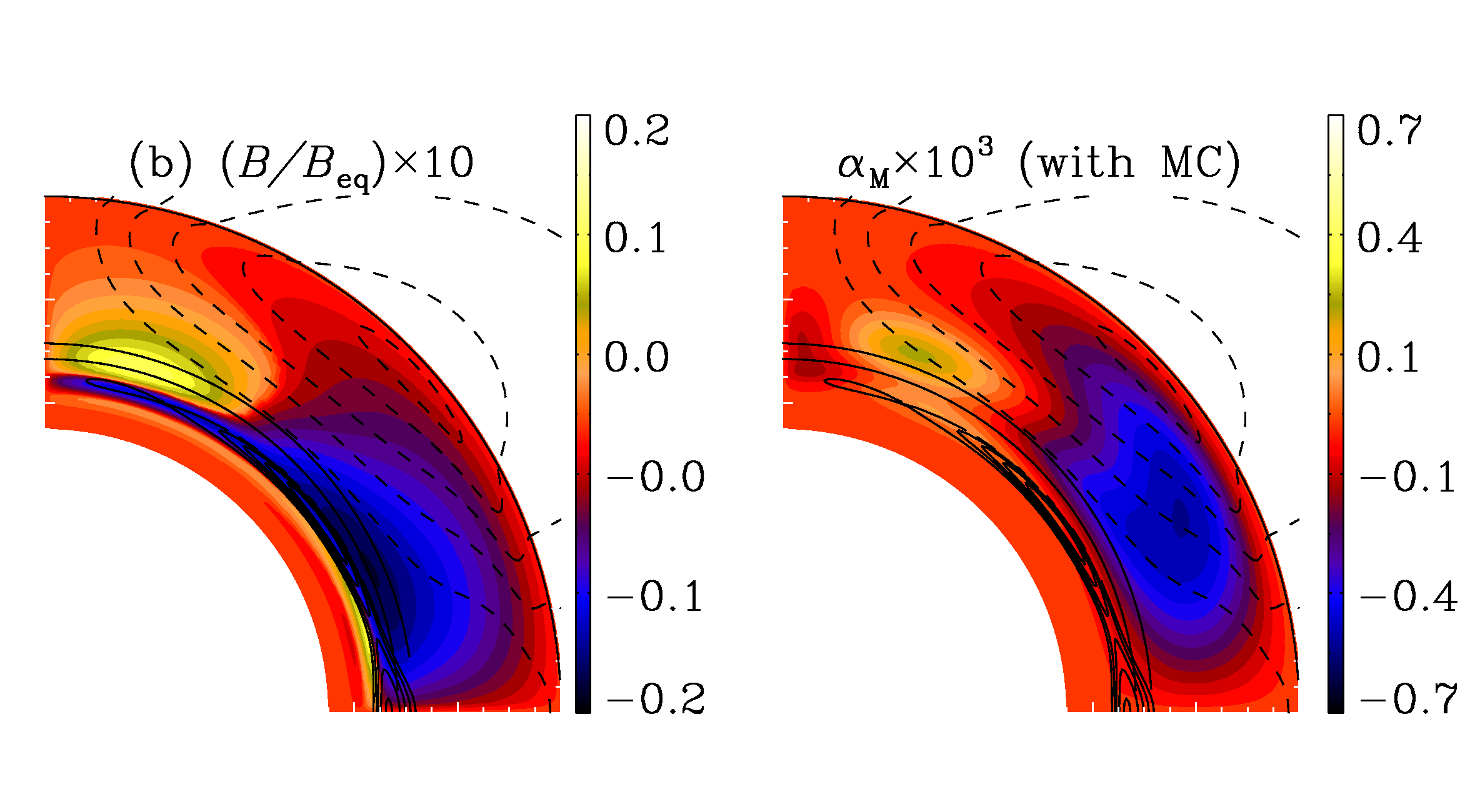
Figure 14: Meridional cross-sections showing the distribution of toroidal field and $\alpha_{M}$ for a Babcock-Leighton dynamo with MC and diffusive helicity fluxes for $R_{\rm m}=2\times 10^{3}$ at two different epochs. The streamlines of the positive and negative poloidal field are shown by solid and dashed lines respectively.

4 Conclusions

We have performed calculations for $\alpha\Omega$ dynamos in a spherical shell for spatially segregated $\alpha$ and $\Omega$ source regions. The two classes of models we have studied resemble the Parker’s interface dynamo and the Babcock-Leighton dynamo.

In agreement with earlier work, it is not possible to escape catastrophic quenching by merely separating the regions of shear and $\alpha$-effect. The saturation value of magnetic energy decreases as $\sim R_{\rm m}^{-1}$ for both dynamical quenching and the algebraic quenching with $g_{\alpha}=R_{\rm m}$ for the simple two layer model without meridional circulation (Fig. 5). However we find that a richer dynamical behaviour emerges for the cases with dynamical $\alpha$ effect, in terms of parity fluctuations and appearance of ‘secondary’ dynamos (Fig. 8, 9). We do not see evidence for chaotic behaviour in the time series of magnetic energy since the dynamo period and the saturation energy remains fairly constant. However this may not be the case in presence of diffusive helicity fluxes which introduce further complexity to the system. Addition of diffusive helicity fluxes relaxes the catastrophic $R_{\rm m}^{-1}$ dependence of the saturation magnetic energy (Fig. 10a, 12). An interesting ‘side-effect’ of diffusive helicity fluxes is the appearance of poleward propagating secondary dynamos. However, because of the lack of scale separation between the mean field and the forcing scale of the helical turbulence we refrain from interpreting this in terms of the poleward migration seen in the Sun. It remains to explore the role of the solar wind, coronal mass ejections which might help in throwing out the small scale helicity from the Sun and thus alleviate catastrophic quenching. The effects of Vishniac & Cho fluxes have been investigated and were found to be of secondary importance compared to diffusive helicity fluxes for $\alpha\Omega$ mean field dynamos (Guerrero, Chatterjee & Brandenburg 2010).

When both the meridional circulation and the diffusive helicity fluxes are artificially shut off in the helicity evolution equation, the dynamo fails to reach significant saturation values, as expected (Fig. 12). It is interesting that the Babcock-Leighton dynamos, where $\alpha$ is concentrated only in a narrow layer at the surface, also produce considerable helicity inside the convection zone when the dynamical quenching (Eq. 6) is employed (Fig. 13, 14).

We have to be cautious about using dynamical quenching equation for dynamo numbers not very large compared to the critical dynamo number. For highly supercritical $\alpha$, the behaviour of the system begins to be governed by $\alpha_{\rm M}$. We would expect that the magnetic field should affect all the turbulent coefficients including both $\alpha$ and $\eta$. However for this analysis we have not included an equation for the variation for $\eta_{\rm t}$. This is justified for the simple two layer model with a lower $\eta_{\rm t}$ in the region of production of strong toroidal fields and a higher $\eta_{\rm t}$ in the region of weaker poloidal fields. It may also be noted that by quenching the diffusivity inversely with the magnetic energy in a nonlinear dynamo model, Tobias (1996) was able to produce a bonafide interface model where the magnetic field was restricted to a thin layer at an interface between a layer of shear and cyclonic turbulence. However none of the previous interface models have used the dynamical quenching equation.

Unfortunately the direct numerical simulations have not yet reached the modest Reynolds numbers used in this paper ($\sim 10^{4}$) which are still much lower than the astrophysical dynamos. To verify if the equation for dynamical quenching works in the same way as in $\alpha^{2}$ dynamos, we need to embark upon systematic comparisons between DNS with shear and convection and mean field modelling for $\alpha\Omega$ dynamos.

- (1) Archontis, V., Dorch, S. B. F., & Nordlund, Å. 2003, A&A, 397, 393
- (2) Blackman, E. G., & Brandenburg, A. 2002, ApJ, 579, 359
- (3) Blackman, E. G., & Field, G. B. 2000, MNRAS, 318, 724
- (4) Brandenburg, A., & Subramanian, K. 2005, AN, 326, 400
- (5) Brandenburg, A., Bigazzi, A., & Subramanian, K. 2001, MNRAS, 325, 685
- (6) Brandenburg, A., Candelaresi, S., & Chatterjee, P. 2009, MNRAS, 398, 1414
- (7) Brandenburg, A., Rädler, K.-H., & Schrinner, M. 2008, A&A, 482, 739
- (8) Cattaneo, F., & Hughes, D. W. 1996, PRE, 54, R4532
- (9) Charbonneau, P., 2005, Living Rev. in Solar Phys., 2, http://www.livingreviews.org/lrsp-2005-2
- (10) Chatterjee, P., Nandy, D., & Choudhuri, A. R. 2004, A&A, 427, 1019
- (11) Chatterjee, P., Brandenburg, A. and Guerrero, G. 2010, Geophys. Astrophys. Fluid Dyn. (accepted), preprint: NORDITA-2010-34
- (12) Choudhuri, A. R., Schüssler, M., & Dikpati, M. 1995, A&A, 303, L29
- (13) Covas, E., Tworkowski, A., Brandenburg, A., & Tavakol, R. 1997, A&A, 317, 610
- (14) Dikpati, M., & Choudhuri, A. R. 1994, A&A, 291, 975
- (15) Dikpati, M., & Charbonneau, P. 1999, ApJ, 518, 508
- (16) Durney, B. R. 1995, Sol. Phys., 160, 213
- (17) Guerrero, G., & de Gouveia Dal Pino, E. M. 2008, A&A, 485, 267
- (18) Guerrero, G., Chatterjee, P., & Brandenburg, A. 2010, MNRAS, submitted, arXiv:1005.4818
- (19) Jepps, S. A. 1975, JFM, 67, 625
- (20) Jouve, L., Brun, A. S., Arlt, R., Brandenburg, A., Dikpati, M., Bonanno, A., Käpylä, P. J., Moss, D., Rempel, M, Gilman, P., Korpi, M. J., & Kosovichev, A. G. 2008, A&A, 483, 949
- (21) Käpylä, P. J., Korpi, M. J. & Brandenburg, A. 2008, A&A, 491, 353
- (22) Kleeorin, N., & Rogachevskii, I. 1999, PRE, 59, 6724
- (23) Kleeorin, N., Moss, D., Rogachevskii, I., & Sokoloff, D. 2000, A&A, 361, L5
- (24) MacGregor, K. B., & Charbonneau, P. 1997, ApJ, 486, 484
- (25) Markiel, J. A., & Thomas, J. H. 1999, ApJ, 523, 827
- Mitra et al. (2010) Mitra, D., Candelaresi, S., Chatterjee, P., Tavakol, R. & Brandenburg, A. 2010, Astron. Nachr., 331, 130
- (27) Ossendrijver, M. , Stix, M. , Brandenburg, A. , & Rüdiger, G. 2002, A&A, 394, 735
- (28) Parker, E. N. 1955, ApJ, 122, 293
- (29) Parker, E. N. 1993, ApJ, 408, 707
- (30) Petrovay, K. & Kerekes, A. 2004, MNRAS, 351, L59
- (31) Shukurov, A., Sokoloff, D., Subramanian, K., & Brandenburg, A. 2006, A&A, 448, L33
- (32) Spiegel, E. A. & Zahn, J.-P. 1992, A&A, 265, 106
- (33) Subramanian, K., & Brandenburg, A. 2006, ApJ, 648, L71
- (34) Sur, S., Shukurov, A. & Subramanian, K. 2007, MNRAS, 377, 874
- (35) Tobias, S. M., 1996, ApJ, 467, 870
- (36) van Ballegooijen, A. A., Choudhuri, A.,R. 1988, ApJ, 333, 965
- (37) Vainshtein, S. I., & Cattaneo, F. 1992, ApJ, 393, 165
- (38) Vishniac, E. T., & Cho, J. 2001, ApJ, 550, 752
- (39) Zhang, H., Sokoloff, D., Rogachevskii, I., Moss, D., Lamburt, V., Kuzanyan, K., & Kleeorin, N. 2006, MNRAS, 365, 276