Wavelet and $R/S$ analysis of the X-ray flickering of cataclysmic variables

Abstract

Context. Recently, wavelets and $R/S$ analysis have been used as statistical tools to characterize the optical flickering of cataclysmic variables.

Aims. Here we present the first comprehensive study of the statistical properties of X-ray flickering of cataclysmic variables in order to link them with physical parameters.

Methods. We analyzed a sample of 97 X-ray light curves of 75 objects of all classes observed with the XMM-Newton space telescope. By using the wavelets analysis, each light curve has been characterized by two parameters, $\alpha$ and $\Sigma$, that describe the energy distribution of flickering on different timescales and the strength at a given timescale, respectively. We also used the $R/S$ analysis to determine the Hurst exponent of each light curve and define their degree of stochastic memory in time.

Results. The X-ray flickering is typically composed of long time scale events $(1.5\la\alpha\la 3)$, with very similar strengths in all the subtypes of cataclysmic variables $(-3\la\Sigma\la-1.5)$. The X-ray data are distributed in a much smaller area of the $\alpha-\Sigma$ parameter space with respect to those obtained with optical light curves. The tendency of the optical flickering in magnetic systems to show higher $\Sigma$ values than the non-magnetic systems is not encountered in the X-rays. The Hurst exponents estimated for all light curves of the sample are larger than those found in the visible, with a peak at 0.82. In particular, we do not obtain values lower than 0.5. The X-ray flickering presents a persistent memory in time, which seems to be stronger in objects containing magnetic white dwarf primaries.

Conclusions. The similarity of the X-ray flickering in objects of different classes together with the predominance of a persistent stochastic behavior can be explained it terms of magnetically-driven accretion processes acting in a considerable fraction of the analyzed objects.

1 Introduction

Cataclysmic variables (CVs) are binary systems in which a late-type secondary star transfers matter onto a white dwarf (WD) primary. The accretion configuration is different depending on the magnetic field strength of the WD. In non-magnetic systems the accretion disk extends down to the WD surface, while a truncated disk may form in moderately magnetic CVs or may not be present at all in strongly magnetized systems (see Warner 1995 for a review).

Owing to the gravitational potential of the compact primary, the accretion of matter produces a non-negligible flux of X-rays. The mechanism responsible for this emission in non-magnetic CVs during quiescence is the shock heating that acts in the boundary layer between the accretion disk and the WD surface (Patterson & Raymond 1985a, b), while in magnetic systems X-rays are emitted by a standing shock above the magnetic poles of the WD (Aizu 1973). In the latter case the X-ray flux is higher, which makes the magnetic systems the brightest X-ray CVs.

Cataclysmic variables are subdivided into three main classes: novae (classical and recurrent), dwarf novae (DNe) and nova-like (NL) systems. In addition, there is a class of objects closely related to novae, the so-called super-soft X-ray sources (SSSs), whose members are characterized by a prominent soft spectral component due to thermonuclear burning at the WD surface (see e.g. Orio 1995). A parallel classification can be made considering the strength of the magnetic field $B$ of the primary. In this case we have the non-magnetic systems, the intermediate polars (IPs, $B\sim 5-10$ MG) and the polars ($B\ga 10$ MG).

The X-ray light curves of CVs may exhibit a variety of modulations. Periodic coherent modulations due to occultations of the emitting regions can be produced by the orbital motion or by the rotation of the WD. For magnetic systems periodic modulations can also be ascribed to absorption effects produced in the magnetically-confined accretion flow [“columns” in polars (Cropper 1990), “curtains” in IPs (Rosen et al. 1988)]. Besides this persistent variability, CVs may also show quasi-periodic oscillations (QPOs) in both the soft and hard X-ray bands as well as completely stochastic brightness variations, which are usually identified with the term “flickering” (see Kuulkers et al. 2006, and references therein).

Flickering is generally constituted by a sequence of random flares with typical timescales ranging from a few seconds to a few minutes. This phenomenon has been observed in the X-ray light curves of CVs of all classes. For example, observations with the HEAO-1 satellite allowed the discovery of soft X-ray flickering in the polar prototype AM~Her (Szkody et al. 1980), as well as hard X-ray aperiodic variability in the DN SS~Cyg during quiescence (Cordova et al. 1984). Flickering at timescales of $\sim 10$ s was detected in the NL TT~Ari using both Einstein (Jensen et al. 1983) and ASCA (Baykal & Kiziloğlu 1996) data. Rapid aperiodic fluctuations were discovered in the light curves of a bunch of CVs also using ROSAT observations (Holcomb et al. 1994; Rosen et al. 1995; Buckley et al. 1998). A common observational feature is that X-ray flickering shows a continuous power law frequency spectrum, as it does in the visible region. A correlation between the time scale of the X-ray flickering activity and that detected in simultaneous optical observations was found in a number of CVs of different classes, e.g. the IP system V795~Her (Rosen et al. 1995), the polar EF~Eri (Watson et al. 1987), the VY~Scl star TT Ari (Jensen et al. 1983), the old nova V603~Aql (Drechsel et al. 1983) and in the DNe SS Cyg and U~Gem (Cordova et al. 1984). This observational evidence has been commonly explained as the result of reprocessing of the X-ray flickering energy.

The properties of flickering have been studied for a long time, especially in the visible region of the electromagnetic spectrum. However, the origin of optical flickering is still uncertain, although there is plenty of evidence that it has to be related to the accretion process. It is very likely that the location of its source should be restricted either to regions very close to the WD, like the innermost part of the disk, or the hot spot (see Bruch 1992 for a thorough discussion). The connection between X-ray flickering and the accretion onto the WD, instead, is evident. For highly magnetic CVs, the rapid soft X-ray flares often detected in their light curves could been explained as the result of a bombardment of the WD surface by random inhomogeneous structures (“blobs”) present in the accretion streams (Kuijpers & Pringle 1982). For instance, the features observed in the light curves of the polar V1309~Ori (de Martino et al. 1998; Schwarz et al. 2005) and of the asynchronous polar BY~Cam (Ramsay & Cropper 2002), although they are quite peculiar objects, could be explained with this hypothesis. Also the flares observed in the X-ray light curve of the old nova GK~Per, which is an IP, have been interpreted as an indirect indication of blobby accretion (Vrielmann et al. 2005).

In general, it is often possible to obtain some information about the flickering from the observations of a single object. However, as this is a stochastic process in time, it can be better studied by means of its statistical properties. Fritz & Bruch (1998, hereafter FB98) carried out a statistical analysis of the optical flickering of a large sample of CVs based on the wavelet analysis (Daubechies 1992) of their light curves. They represented the properties of flickering in a two-dimensional parameter space and showed that CVs of different classes tend to occupy different regions of this space. Later Tamburini et al. (2009, hereafter TDB09) used the $R/S$ rescaled range analysis (Hurst 1951; Hurst et al. 1965) for the first time as a complementary tool to characterize the degree of persistence/anti-persistence of the white light flickering of the IP-class CV V709~Cas. Motivated by the interesting results presented in these works, we have therefore used the same statistical techniques to study the X-ray flickering properties of CVs as a whole as well as a function of their individual classes to link them with physical parameters.

2 The $\alpha-\Sigma$ parameter space and the Hurst exponent

A light curve is represented by a set of data points taken at times $t_{1},\ldots,t_{N}$. We assume that the difference between two consecutive times in the sequence is a constant $\Delta t$, which usually coincides with the binning time. The calculation of the wavelet transform roughly consists in decomposing the analyzed signal into a sequence of wavelets all with a general predefined shape (the mother wavelet), but different positions in time and different scalings. The result is a two-dimensional set with the coefficients $c_{s,k}$, where $k=1,\cdots,N$ is the time index and $s$ is related to the timescale $t_{s}=2^{s}\Delta t$. It is then possible to calculate the quantity

$$S^{\prime}(t_{s})=\frac{2^{s}}{N}\sum_{k}c_{s,k}^{2}\,,$$ (1)

which represents a measure of the variance of the wavelet coefficients on different timescales. The logarithmic plot of $S^{\prime}(t_{s})$ as a function of $t_{s}$ is called scalegram (Scargle et al. 1993). Fritz & Bruch (1998) introduced a normalized version of the scalegram,

$$S(t_{s})=S^{\prime}(t_{s})\frac{N\Delta t}{\sum_{s,k}c_{s,k}^{2}}\,,$$ (2)

and applied it to a large sample of optical flickering light curves of CVs of different classes. It turned out that almost all scalegrams so obtained were approximately linear functions of $t_{s}$, thus permitting a complete representation of the flickering properties with two parameters: the slope $\alpha$ with respect to the $\log t_{s}$ axis, which also indicates whether slow or rapid light fluctuations dominate the stochastic time series, and the strength at a given timescale $t_{\mathrm{ref}}$, $\Sigma=\log S(t_{\mathrm{ref}})$. Surprisingly, their results indicate that different subtypes of CVs tend to occupy specific regions of the $\alpha-\Sigma$ parameter space. This subdivision shows a remarkably small overlap for magnetic NL systems.

The linearity of the scalegrams also reveals that the flickering has the intriguing property of being self-similar on a wide range of timescales. Self-similarity is a statistical property of an observable $x(t)$ and is typical of the so-called fractional Brownian motions (Mishura 2008). In general, $x(t)$ is said to be self-similar for any scale magnification $\lambda$ if the following relation holds:

$$x(\lambda t)=\lambda^{H}x(t)\,.$$ (3)

The $H$ parameter, called the Hurst exponent, is of fundamental importance in defining the statistical properties of a physical process. In dynamical systems, where $x(t)$ is a function of a continuous variable $t$, the Hurst exponent characterizes the stochastic memory in time of a random process, because it expresses the tendency of the first derivative of $x(t)$ to change sign. A process is said to be persistent when $H>1/2$, while an exponent $H<1/2$ indicates anti-persistence. In the particular case $H=1/2$, the process shows a random uncorrelated behavior with no stochastic memory in time (Peters 1994).

From an observational point of view, $x(t)$ is represented by a time series with a discrete time domain. Yet the self-similarity relation expressed by Eq. 3 is still valid, as are the properties of the $H$ parameter. One of the most efficient statistical method used to estimate the Hurst exponent of a time series is the $R/S$ analysis. The $R/S$ analysis is non-parametric, in the sense that there are no specific assumptions or requirements for the distribution of the observables. Moreover, it has been shown to be robust even in the presence of a discrete noise level (Chamoli et al. 2007).

Given a set of observables $x(t)$ with $0\leq t\leq T$, the $R/S$ analysis consists in subdividing the data set in intervals of length $\tau$ and evaluating the range

$$R(\tau)=\max[X(t,\tau)]-\min[X(t,\tau)]$$ (4)

and the standard deviation

$$S(\tau)=\sqrt{\frac{\sum_{k=1}^{\tau}{\left[x(t)-{\left<x\right>}_{\tau}\right]}^{2}}{\tau}}\,,$$ (5)

where ${\left<x\right>}_{\tau}$ is the average value of the observable in each sub-interval and $X(t,\tau)=\sum_{k=1}^{t}\left[x(k)-\left<x\right>_{\tau}\right]$. The average value of $\left<R/S\right>_{\tau}=\left<R(\tau)/S(\tau)\right>$, i.e. a quantity that describes the “distance” covered by the observable in units of the local standard deviation, is then calculated for each sub-interval of equal length $\tau$. For a self-similar process, it can be shown that

$$\left<R/S\right>_{\tau}\sim\tau^{H}\,.$$ (6)

Hence, the Hurst exponent is represented by the slope of the linear relation between $\log\tau$ and $\log\left<R/S\right>_{\tau}$.

It has been also demonstrated that the time-averaged wavelet coefficients depend on the scale parameter following a power law with exponent $H+1/2$ (Simonsen et al. 1998). Therefore, the variance of the wavelet coefficients averaged with respect to the $k$ time index must satisfy the relation

$${\left<c_{s,k}\right>}_{k}\sim 2^{\beta s}\,,$$ (7)

where $\beta=2H+1$ (Gao et al. 2003). Because of this property, TDB09 proposed to use the $R/S$ analysis as a complementary tool to characterize the stochastic properties of flickering by calculating the parameter $\alpha$ through the determination of the Hurst exponent $H$.

3 Data analysis

In order to obtain a homogeneous sample of X-ray light curves, we used data collected with the EPIC cameras (pn, MOS1 and MOS2) onboard the XMM-Newton telescope (Jansen et al. 2001), which provide both good timing accuracy and high sensitivity. The latter property is of particular importance when dealing with DNe in quiescence, which are typically faint in the X-ray band. Moreover, thanks to the high spacecraft orbit, XMM-Newton is an ideal observatory to achieve long [up to $\sim 40\mbox{ hr}$ (Barré et al. 1999)] uninterrupted observations and therefore obtain good quality light curves for the $R/S$ analysis.

We used the Catalogue of Cataclysmic Binaries, Low-Mass X-Ray Binaries and Related Objects, edition 7.11  (Ritter & Kolb 2003), to select all CVs observed with XMM-Newton and obtain their J2000 coordinates. We then retrieved all publicly available data containing processed light curves of these objects from the XMM-Newton Science Archive (Arviset et al. 2002). Because the largest part of the observations were pointed, many of the X-ray sources could be safely identified with the corresponding object in the catalog. However, a visual check of the automatic identification process was applied for those data that were not pointed, to exclude spurious sources from our sample. In this way we found 116 light curves of X-ray sources positively ascribed to CVs. These light curves, as part of the pipeline products obtained from observations with the EPIC cameras operated either in imaging or timing mode, were automatically extracted in the 0.2–12 keV energy range, background-subtracted and binned to obtain a sufficiently good S/N ratio for each bin. We did not apply the heliocentric correction, because in all cases it is of the order of 0.1 s at most and therefore is negligible compared to the binning time that is always longer than 10 s.

The quality of the light curves was then checked to select only those suitable for the statistical analysis. As a first step, although a screening for high background radiation was already applied to the data during the processing at SSC, we carefully checked the background status during each observation and discarded all data subjected to high background contamination. When large gaps were present, the resulting screened light curves were further reduced to have a continuous coverage of $N>128$ points and therefore at least six points in the scalegrams. This also gave reliable results from the $R/S$ analysis (Katsev & L’Heureux 2003). Furthermore, for some objects the count rate was too low $(<0.1\mbox{ counts s}^{-1})$ and the corresponding light curves were discarded. After this selection procedure, our final sample constituted a total of 97 light curves of 75 objects: 23 light curves of 20 DNe, 60 light curves of 46 NL systems, 9 light curves of 5 novae and 5 light curves of 4 SSSs (see Table 1).

The binning time applied during the pipeline processing at SSC has a lower limit of 10 s for the brightest objects and is short enough to sufficiently sample the flickering with short timescales. But this binning time does not allow us to include in the statistical analysis the very rapid flickering (timescale of $1-5\mbox{ s}$) that might be present in many CVs, especially those hosting strongly magnetic WDs.

The actual amplitude of the flickering at these very short timescales could be strongly affected by the shot noise of the EPIC cameras, whose amplitude is roughly proportional to the square root of the binning time $\Delta t$ assuming a pure Poissonian noise and a constant count rate within $\Delta t$. As a result, the scalegrams of all light curves would show a flattening at those short timescales, regardless of the class of the object. With the adopted binning time we expect to avoid this undesired behavior, which might bias the real statistical properties of flickering.

For each light curve we calculated the $c_{s,k}$ coefficients provided by a discrete wavelet transform algorithm with a Coiflet C12 mother wavelet and obtained the corresponding scalegrams. Then, we derived the $\alpha$ parameters by linearly fitting the data points at all time scales, while $\Sigma$ was calculated at $t_{\mathrm{ref}}=0.05\mbox{ hr}$. The wavelet type and the reference time adopted in our analysis were chosen to allow a direct comparison with the results of TDB09 and FB98 obtained for the flickering in the visible region. None of the analyzed scalegrams showed any tendency to be flat at small scales, thus indicating that the S/N ratio was high enough.

The Hurst exponent was estimated using the $R/S$ analysis and considering all the sub-intervals of each light curve containing a number of data points in the interval $[10,N]$. The lower limit was chosen to obtain statistically significant mean values and standard deviations.

To obtain the $H$ parameter we had to perform a linear fit of all the data points appearing in the $\log\tau-\log\left<R/S\right>_{\tau}$ plane. However, for almost all light curves we found that there was not just one linear regime of the rescaled range, thus indicating the presence of different scaling laws at different time scales. Examples of this behavior are shown in Fig. 1 with the data obtained from the $R/S$ analysis of the X-ray light curves of GK Per, CP~Pup and FO~Aqr. While the curve of the latter object is almost linear at all scales, for the other two there are two different regimes below and above $\log(\tau[\mbox{hr}])\sim-0.5$. An investigation of this peculiar behavior, which is typical of multifractal systems (Stanley & Meakin 1988), is beyond the scope of this paper. Still, the presence of bends in the scaling law is a well known effect that arises when there are periodic signals. Indeed, if a periodic modulation with a period $P$ is present in a self-similar time series, then a break in the initially linear scaling law will appear exactly at $\log P$. Moreover, there will be more than one break if there are many superposed periodic signals (Peters 1994). For those data in the sample that show this phenomenon in the $\log\tau-\log\left<R/S\right>_{\tau}$ plane, the breaks are always found at $\log(\tau[\mbox{hr}])\ga 0.1$ and, therefore, we might expect that they are likely produced by QPOs or by proper dynamical motions of the CV systems. For instance, the curve of CP Pup changes its slope at long time scales (see Fig. 1), where it also shows some oscillations, because of the appearance of the orbital period $\log(P_{\Omega}[\mbox{hr}])=0.167$ of the system.

The estimation of a unique value of the Hurst exponent is not an adequate way to describe the self-similarity properties of a light curve because in this way it is impossible to decouple the different scaling behaviors that might be appearing in different regions of the $\log\tau-\log\left<R/S\right>_{\tau}$ plane (Simonsen 2003). Because we are only interested in the flickering, we estimated the $H$ exponents considering just the linear portion of the rescaled range at small scales, i.e. before the appearance of the first break.

The results of our analysis are shown in Table 1, where the entries of the columns are

1. name of the object;

2. class of the CV (DN = dwarf nova, NL = nova-like, N = nova, SS = super-soft X-ray source);

3. subtype according to Ritter & Kolb 2003 (AC = AM CVn, IP = intermediate polar, P = polar, SU = SU UMa, SW = SW Sex, UG = either U Gem or SS Cyg, UX = UX UMa, VY = VY Scl, WZ = WZ Sge, ZC = Z Cam);

4. observation ID number;

5. date of the observation;

6. instrument with which the light curve has been obtained (PN = EPIC-pn, M1 = EPIC-MOS1, M2 = EPIC-MOS2);

7. net exposure time;

8. binning time;

9. state of the object at the time of the observation, if known (Q = quiescence, O = outburst, H = high-state, L = low state, I = intermediate state, D = decline from nova eruption);

10. mean count rate;

11. $\alpha$ parameter with $1\sigma$ uncertainty;

12. $\Sigma$ parameter with $1\sigma$ uncertainty;

13. Hurst exponent with $1\sigma$ uncertainty.

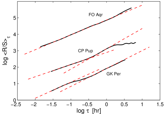
Figure 1: $\log\tau-\log\left<R/S\right>_{\tau}$ graphs obtained from the $R/S$ analysis of the X-ray light curves of three CVs of different classes. The curves of CP Pup and FO Aqr were shifted by 1.5 and 3 respectively along the vertical axis. The dashed lines are linear fits of all linear portions found in each curve.

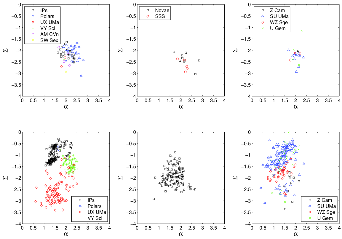
Figure 2: $\alpha-\Sigma$ diagrams of NL systems (left panels), novae and SSSs (central panels) and DNe (right panels). The diagrams in the top row are obtained from the X-ray data analyzed in this work, whereas those in the bottom row are obtained from observations in the visible band (FB98).

4 Results

The diagrams representing the distributions of the $\alpha$ and $\Sigma$ parameters obtained with the wavelet analysis of the X-ray light curves are shown in the upper part of Fig. 2. For comparison, we also plotted the corresponding diagrams obtained by FB98 from the analysis of data in the visible band . The data points were subdivided in three diagrams corresponding to the different classes of CVs and marked with different symbols in function of their subtypes, according to the classification of Ritter & Kolb (2003). We also included SSSs, which was not considered in FB98, because of their affinity with novae and their prominent emission in the soft X-ray domain.

A remarkable result is that all X-ray data points seem to be contained within a small area delimited by $1.5\la\alpha\la 3$ and $-3\la\Sigma\la-1.5$, regardless of the CV class. If we compare the three X-ray diagrams in Fig. 2, we can see that data points belonging to objects of different classes totally overlap within this small region. This reveals a very homogeneous behavior of the X-ray flickering, with just very marginal differences shown in function of the subtype of CVs. Considering only the X-ray data of NL systems, there is a tendency for some members of the polar class to have slightly higher $\alpha$ values than IPs and non-magnetic systems. Moreover, many objects belonging to the NL class show $\Sigma$ values higher than -2, but novae, SSSs and DNe are always found with $\Sigma\la-2$ (with the noticeable exception of SS Cyg). The distribution of the data points of SSSs is very similar to that of novae, although we cannot exclude that this behavior could be due to the incompleteness of the X-ray sample of objects belonging to these groups. Dwarf novae appear to be a rather homogeneous class, as was also pointed out by FB98. Their data points are all located almost in the same region occupied by novae and SSSs, but with an apparently narrower interval of $\alpha$ values.

Some additional information can be inferred from the results of the $R/S$ analysis. The distribution of the Hurst exponents of the whole sample of CVs shown in the left panel of Fig. 3 is quite symmetric, with a peak at $H=0.82$. Moreover, all light curves present values of $H$ higher than 0.6, with no evidence of purely Gaussian processes $(H=0.5)$ acting in any of the objects of the sample. The distribution of $H$ in function of the three classes of CVs (Fig. 3, central panel) is strongly biased by the smaller sample of DNe and novae with respect to the NL systems. We can only say that there is a tendency for the latter to have higher Hurst exponents with respect to the other two classes. If we instead subdivide the whole sample into magnetic and non-magnetic systems by checking the additional sub-classifications reported in the catalog of Ritter & Kolb, the resulting distributions are more statistically significant. Then the two distributions (see Fig. 3, right panel) are peaked almost at the same value $H\sim 0.82$, with magnetic systems showing an evident tail towards higher $H$ and vice-versa for non-magnetic CVs.

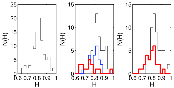
Figure 3: Histograms of the Hurst exponents obtained with the $R/S$ analysis of the X-ray light curves of CVs. The whole sample is presented in the left panel. The central panel shows the distribution of $H$ in function of the class of CVs. The histogram marked with a thin line refers to NL systems, that with an intermediate thickness line refers to DNe and that with a thick line refer to novae and SSSs. In the right panel we report the distribution of $H$ in function of the magnetic nature of the WD primary. The histogram marked with a thin line refers to magnetic CVs, while that with a thick line refers to non-magnetic systems.

5 Discussion

5.1 The visible and X-ray samples

The distribution of the X-ray data points in the $\alpha-\Sigma$ parameter space shows some important differences from that of the visible data, although a direct comparison between the two has to be taken with care. Indeed, the numbers of light curves present in the two samples are very different, about 10 times higher in the FB98 sample than those considered here. However, it is important to note that many of the points in the visible band diagrams refer to the same object, while the points obtained in the X-rays generally correspond to only one light curve per object. Therefore the two samples are comparable in terms of numbers of distinct objects analyzed (73 in the visible and 75 in the X-rays).

Because many of the data points of the the FB98 sample belong to the same object, their distribution in the $\alpha-\Sigma$ parameter space also reflects the temporal variation of the flickering. For this reason, FB98 could analyze the time dependence of the flickering parameter in some CVs and found a significant variability only for the $\alpha$ parameter.

For the X-ray data, it is impossible to do a similar investigation because none of the objects of the sample has a comparable number of light curves taken in different epochs. It is only possible to roughly check the significance of the variations of $\alpha$ and $\Sigma$ parameters by calculating the absolute value of the difference between their maximum and minimum values ($|\Delta\alpha|$ and $|\Delta\Sigma|$) and compare them with the corresponding errors.

All objects with at least two X-ray light curves are listed in Table 1, together with the time $\Delta T$ elapsed between the first and the last observation and the resulting $|\Delta\alpha|$ and $|\Delta\Sigma|$ with $1\sigma$ errors. In general, the variation of the flickering parameters is not statistically significant when compared with the uncertainties. The only exceptions are for those CVs that were observed during a transition between two different states, namely the polar CD~Ind (from high to low state), the novae V2491~Cyg and V4743~Sgr declining to a state of very low emission, and the DN Z~Cha, which was in outburst during the first observation. It seems therefore that the distribution of the X-ray data points of a single CV in the $\alpha-\Sigma$ parameter space does not strongly depend on the time, at least when the object is observed while it is in the same state.

Table 1: Variation of the flickering parameters in some CVs of the X-ray sample.

Object name	$\Delta T$ (d)	$|\Delta\alpha|$	$|\Delta\Sigma|$
AM Her	2.0	$0.29\pm 0.22$	$0.08\pm 0.39$
CD Ind	6.0	$0.78\pm 0.32$	$0.68\pm 0.22$
EI UMa	176.3	$0.19\pm 0.11$	$0.08\pm 0.20$
EX Hya	0.6	$0.03\pm 0.18$	$0.03\pm 0.29$
HT Cas	325.9	$0.04\pm 0.14$	$0.01\pm 0.21$
MR Vel	2.0	$0.03\pm 0.17$	$0.09\pm 0.28$
NY Lup	351.2	$0.07\pm 0.14$	$0.11\pm 0.25$
OY Car	38.4	$0.36\pm 0.13$	$0.21\pm 0.20$
RXJ0704+2625	170.4	$0.11\pm 0.33$	$0.13\pm 0.54$
RXJ2133+5107	38.3	$0.09\pm 0.13$	$0.06\pm 0.23$
V2400 Oph	346.5	$0.01\pm 0.13$	$0.13\pm 0.22$
V2487 Oph	2025.8	$0.11\pm 0.17$	$0.23\pm 0.34$
V2491 Cyg	9.8	$0.48\pm 0.14$	$0.59\pm 0.24$
V4743 Sgr	544.8	$1.16\pm 0.14$	$0.37\pm 0.23$
XY Ari	163.4	$0.22\pm 0.17$	$0.11\pm 0.27$
Z Cha	650.2	$0.05\pm 0.13$	$0.81\pm 0.21$

5.2 The X-ray flickering properties

Taking the issues discussed in Sect. 5.1 into consideration, we can see that the distribution of the X-ray data appears to be much less dispersed than in the visible. The $\alpha$ parameter is found to be positive for all the objects present in the sample, which means that much of the energy is dissipated in long timescale flickering events. However, we do not find $\alpha$ values lower than $\sim 1.5$ for any CV in the X-ray sample. This differs quite remarkably from the distribution of the optical data, where some objects show flickering activity with $\alpha\sim 0.5$. It seems therefore that the X-ray flickering energy is typically dissipated in flares with relatively longer time scales than those in the optical region. Curiously, there seems to be a kind of cutoff at $\alpha\sim 3$ in the X-rays and at $\alpha\sim 2.5$ in the visible, which might imply the existence of an upper limit in the time scale of the flickering independent of the CV class. A more evident difference is detectable between the distributions of the $\Sigma$ parameter that roughly describes the strength of the flickering. Fritz & Bruch (1998) showed that the energy dissipated in the visible flickering spans more than 3 orders of magnitude, independently of the CV class, and seems to be correlated to the subtypes of each class. Instead, the X-ray light curves possess flickering components with very similar strengths. In particular, the evidence found in the visible data that magnetic NL systems have higher $\Sigma$ values than the non-magnetic ones is not detectable in the X-ray data.

All subtypes of NL objects populate very similar regions in the X-ray $\alpha-\Sigma$ parameter space. The tendency of some polars to show slightly higher $\alpha$ values than the other members of the class suggests that the duration of the X-ray flares might be somewhat correlated to the modality of accretion, which also depends on the strength of the magnetic field of the WD.

The $R/S$ analysis demonstrates that the X-ray light curves of CVs have, in general, high values of the Hurst exponent. Therefore, the X-ray flickering has a strong persistent memory in time, including also extreme cases like GK Per (in outburst) and RXJ1312+1736 in which $H$ is close to unity. This is in contrast with the results obtained in the visible band, where TDB09 showed that the distribution of $H$ has a peak at 0.68 and is strongly asymmetric, with a longer tail extending towards lower values of $H$. There the light curves show both persistent $(H>0.5)$ and anti-persistent $(H<0.5)$ behaviors. Note though that TDB09 calculated the Hurst exponents from the $\alpha$ parameters of FB98 using the power law relation of the variance of the wavelet coefficients (Gao et al. 2003). That is why the derived $H$ values might be affected by the presence of multiple scaling laws at the different time scales used by FB98 to calculate $\alpha$.

We also found that magnetic CVs tend to posses higher $H$ values with respect to non-magnetic systems. This implies that the flickering tends to have a more persistent memory in time in those objects where the accretion is driven by WDs with a magnetic field with significantly detectable strengths. As proposed by TDB09, this property could be used as a further method to assess the membership of a CV to a specific class. For instance, we consider LS~Peg, V426~Oph and EI~UMa, whose classification is still uncertain. The properties of the X-ray spectra of these objects are similar to those of of IPs , but their X-ray light curves do not show any strong modulation at the spin period of the WD (Ramsay et al. 2008). However, from our analysis of the X-ray flickering we find $H$ exponents larger than 0.8 in all their light curves (see Table 1), which could support their magnetic nature.

5.3 A possible explanation

It is not straightforward to give an explanation of the difference between the optical and X-ray flickering properties so far described. In CVs hosting an accretion disk we expect a significant contribution to the optical flickering due to reprocessing of X-rays (Suleimanov et al. 2003), because the X-ray radiation is most likely produced very close to the WD primary. If these system were also magnetic, there should be an additional contribution to the optical flickering from the accretion columns. This might explain the higher $\Sigma$ presented in the visible by magnetic NL systems. However, a simple reprocessing process cannot explain the observed difference in polar systems, which do not contain an accretion disk.

Warner (2004) proposed a scenario in which rapid quasi-coherent brightness modulations in CVs with an accretion disk could be of magnetic origin. He then argued that a dominant fraction of apparently non-magnetic systems could host WD primaries with non-negligible fields $(B\la 7\mbox{ MG})$. If we adopt this interpretation, we could expect the X-ray flickering to be connected to a magnetically-driven accretion process in the majority of the objects. This might explain why we find in the X-ray band a strong similarity among all the classes of CVs. On the other hand, the appearance of a distinction in the visible between the magnetic and the (supposed) non-magnetic systems with accretion disk could be explained, apart from reprocessing, if WDs with higher magnetic fields somehow enhance the optical flickering through processes related to magneto-hydrodynamical turbulence (King et al. 2004; Dobrotka et al. 2009).

The link between magnetic accretion and X-ray flickering could explain not only that magnetic CVs tend to have higher Hurst exponents, but also the evidence that it is, on average, higher in the X-rays than in the optical region. An argument in favor of this interpretation comes from studies of artificially generated magnetized plasma, which is a state very similar to that of the matter within an accretion flow in the proximity of the WD. It has been experimentally found that edge fluctuations of plasma in several magnetic confinement devices possess a long-range time correlation, showing values of $H$ between 0.62 and 0.75 (see e.g. Carreras et al. 1999; Gilmore et al. 2002). The same behavior has been noticed in turbulent plasma by studying the statistics of pulsed phenomena very similar to the blobs supposed to be generating the X-ray flickering in polars or in IPs with disk-overflow accretion (Dendy & Chapman 2006; Sandberg et al. 2009).

6 Conclusions

We have used the wavelets and the $R/S$ analysis as statistical tools to characterize the flickering in a sample of 97 X-ray light curves of CVs of all classes.

In general, the distribution of the X-ray data points in the $\alpha-\Sigma$ parameter space is almost independent of the class and, therefore, quite different from that in the visible. The $\alpha$ parameters are all contained in the range $1.5\la\alpha\la 3$. This implies that the dissipation of the flickering energy occurs typically in long time scale flares. Moreover, the strength of the X-ray flickering is found to vary in the region $-3\la\Sigma\la-1.5$, which is much smaller than that found in the optical region. There is no evidence for magnetic NL systems to have higher $\Sigma$ values than the non-magnetic systems. The different behavior in the visible region and in the X-rays could be explained assuming that part of the optical flickering in system harboring an accretion disk could be originated by other slower components such as trailing waves.

All objects in our sample show values of the Hurst exponent higher than 0.5, with a peak of the distribution at $H=0.82$. The predominance of a persistent stochastic behavior can be ascribed to a magnetically-driven accretion process acting in the majority of the CVs considered here. In particular, the result obtained for magnetic CVs clearly depicts the behavior of a plasma trapped by the magnetic field in the accretion streams.

However, it must be pointed out that the sample of the X-ray light curves analyzed here is still not large enough to allow us to draw firm conclusions. Therefore, the analysis of further data collected in future X-ray observations will permit us to overcome possible selection effects and to better define the statistical properties of the flickering. On the other hand, a larger sample of polar systems analyzed in the optical region would allow us to verify our suggestion that the observed properties of X-ray flickering are intimately related to magnetically-driven accretion processes.

As a final remark, it would have been interesting to use the method proposed by TBD09 to calculate the Hurst exponent from the $\alpha$ parameter (or vice-versa) and quantitatively demonstrate the impact of that procedure. However, it was not possible to do it with the X-ray data because for the vast majority the of the objects in the sample the $R/S$ analysis has been typically stopped at a timescale comparable to the second or third “octave” of the corresponding scalegrams. For this reason, the $H$ values obtained with the two methods are not comparable because either they refer to different timescales maybe including multiple Hurst exponents, or the $\alpha$ parameter is obtained by linearly fitting just two or three points, which is not reliable.

1

Table 2: Results of the wavelet and $R/S$ analysis of the sample of X-ray light curves (see text for details).

Object	Class	Subt.	OBSID	Date obs.	Instr.	Exp. (s)	Bin (s)	State	Mean rate $(\mbox{cts s}^{-}{1})$	$\alpha$	$\Sigma$	$H$
AB Dra	DN	ZC	0111971601	2002-10-06	PN	10060	10	Q	$2.256\pm 0.014$	$2.12\pm 0.06$	$-2.03\pm 0.11$	$0.836\pm 0.005$
AE Aqr	NL	IP	0111180201	2001-11-07	PN	13930	10	Q	$7.253\pm 0.022$	$2.39\pm 0.08$	$-2.35\pm 0.14$	$0.862\pm 0.008$
AI Tri	NL	P	0306841001	2005-08-22	PN	19900	50	H	$0.466\pm 0.004$	$2.32\pm 0.23$	$-2.50\pm 0.34$	$0.842\pm 0.008$
AM Her	NL	P	0305240401	2005-07-25	M1	9290	10	I	$3.782\pm 0.020$	$2.47\pm 0.12$	$-2.10\pm 0.21$	$0.835\pm 0.005$
			0305240501	2005-07-27	M1	7690	10	I	$4.145\pm 0.023$	$2.18\pm 0.18$	$-2.18\pm 0.32$	$0.795\pm 0.003$
AN UMa	NL	P	0109461701	2002-05-01	M1	7260	20	H	$0.416\pm 0.007$	$2.09\pm 0.13$	$-2.08\pm 0.22$	$0.805\pm 0.004$
AO Psc	NL	IP	0009650101	2001-06-09	M1	40830	10	Q	$1.784\pm 0.006$	$2.07\pm 0.23$	$-1.99\pm 0.40$	$0.852\pm 0.009$
BY Cam	NL	P	0109460901	2001-08-26	M1	5770	10	H	$1.534\pm 0.016$	$2.08\pm 0.16$	$-1.98\pm 0.29$	$0.739\pm 0.003$
CAL83	SS		0123510101	2000-04-23	PN	10020	10		$4.363\pm 0.020$	$2.17\pm 0.16$	$-2.42\pm 0.29$	$0.679\pm 0.003$
CAL87	SS		0153250101	2003-04-18	PN	76760	20		$1.721\pm 0.004$	$2.21\pm 0.19$	$-2.94\pm 0.29$	$0.660\pm 0.008$
CD Ind	NL	P	0111250101	2002-03-27	PN	13260	10	H	$3.946\pm 0.017$	$2.30\pm 0.10$	$-2.07\pm 0.17$	$0.815\pm 0.002$
			0111251401	2002-03-28	PN	8650	10	H	$3.194\pm 0.019$	$2.28\pm 0.15$	$-2.01\pm 0.26$	$0.824\pm 0.002$
			0111251501	2002-03-29	PN	13260	10	I	$2.138\pm 0.012$	$2.14\pm 0.08$	$-1.91\pm 0.13$	$0.823\pm 0.003$
			0111251601	2002-03-30	PN	13250	10	I	$2.815\pm 0.014$	$2.02\pm 0.12$	$-1.77\pm 0.21$	$0.910\pm 0.002$
			0111251801	2002-03-31	PN	14020	10	I	$2.048\pm 0.012$	$2.24\pm 0.03$	$-1.80\pm 0.06$	$0.859\pm 0.002$
			0111251901	2002-04-01	PN	14070	30	I	$0.502\pm 0.005$	$2.79\pm 0.29$	$-2.42\pm 0.46$	$0.822\pm 0.003$
			0111251701	2002-04-02	PN	14320	40	I	$0.470\pm 0.005$	$2.26\pm 0.14$	$-2.48\pm 0.21$	$0.833\pm 0.004$
CE Gru	NL	P	0109463501	2001-10-31	PN	7616	40	H	$0.496\pm 0.010$	$2.53\pm 0.20$	$-2.47\pm 0.34$	$0.792\pm 0.008$
CP Pup	N		0304010101	2005-06-04	PN	49960	20	Q	$1.099\pm 0.004$	$2.16\pm 0.12$	$-2.49\pm 0.19$	$0.747\pm 0.003$
CR Boo	DN	SU	0202890201	2003-12-28	PN	20100	30	Q	$0.730\pm 0.006$	$2.14\pm 0.20$	$-2.72\pm 0.30$	$0.701\pm 0.007$
DW UMa	NL	SW	0142970101	2003-10-18	PN	24000	160		$0.104\pm 0.002$	$2.00\pm 0.55$	$-2.95\pm 0.76$	$0.776\pm 0.007$
EI UMa	NL	IP	0111971301	2002-05-10	PN	4700	10	Q	$6.191\pm 0.036$	$2.27\pm 0.07$	$-2.14\pm 0.13$	$0.847\pm 0.001$
			0111971701	2002-11-02	PN	8270	10	I	$6.368\pm 0.027$	$2.09\pm 0.08$	$-2.21\pm 0.14$	$0.865\pm 0.002$
EP Dra	NL	P	0109464501	2002-10-18	PN	17600	20	H	$0.449\pm 0.005$	$2.43\pm 0.10$	$-1.84\pm 0.17$	$0.849\pm 0.004$
EX Hya	NL	IP	0111020101	2000-07-01	M1	43590	10	Q	$6.017\pm 0.011$	$2.35\pm 0.12$	$-2.52\pm 0.21$	$0.804\pm 0.001$
			0111020201	2000-07-01	M1	35060	10	Q	$6.075\pm 0.013$	$2.32\pm 0.13$	$-2.49\pm 0.21$	$0.792\pm 0.001$
EV UMa	NL	P	0109462201	2001-12-08	PN	5040	20	H	$1.714\pm 0.018$	$2.61\pm 0.30$	$-2.33\pm 0.52$	$0.883\pm 0.010$
FO Aqr	NL	IP	0009650201	2001-05-12	M1	36010	10	H	$0.664\pm 0.004$	$2.03\pm 0.06$	$-1.64\pm 0.10$	$0.793\pm 0.002$
GD552	DN	WZ	0301830301	2005-06-18	M1	27300	20	Q	$0.307\pm 0.003$	$1.98\pm 0.09$	$-2.12\pm 0.14$	$0.713\pm 0.003$
GG Leo	NL	P	0109461401	2002-05-13	M1	7840	20	H	$0.391\pm 0.007$	$2.47\pm 0.27$	$-2.14\pm 0.46$	$0.796\pm 0.006$
GK Per	N	IP	0154550101	2002-03-09	PN	29520	10	O	$10.745\pm 0.019$	$2.23\pm 0.15$	$-2.11\pm 0.25$	$0.985\pm 0.002$
GP Com	NL	AC	0017940101	2001-01-03	PN	51270	10	L	$2.040\pm 0.006$	$2.09\pm 0.07$	$-2.17\pm 0.11$	$0.769\pm 0.003$
HP Lib	NL	AC	0202890101	2004-01-28	PN	20100	30	H	$0.553\pm 0.005$	$1.92\pm 0.19$	$-2.49\pm 0.30$	$0.722\pm 0.002$
HS Cam	NL	P	0143430101	2003-10-13	PN	14650	10		$1.879\pm 0.011$	$2.51\pm 0.12$	$-1.67\pm 0.20$	$0.875\pm 0.003$
HT Cam	NL	IP	0144840101	2003-03-24	M1	40480	20	Q	$0.412\pm 0.003$	$1.77\pm 0.18$	$-2.18\pm 0.28$	$0.788\pm 0.006$
HT Cas	DN	SU	0111310101	2002-08-20	PN	47980	20	Q	$0.937\pm 0.004$	$1.95\pm 0.06$	$-2.17\pm 0.09$	$0.834\pm 0.004$
			0152490201	2003-07-12	PN	42600	30	Q	$0.722\pm 0.004$	$1.98\pm 0.13$	$-2.16\pm 0.19$	$0.846\pm 0.007$
HU Aqr	NL	P	0110860101	2002-05-16	M1	37658	30	I	$0.142\pm 0.002$	$1.89\pm 0.16$	$-1.85\pm 0.26$	$0.934\pm 0.012$
IX Vel	NL	UX	0111971001	2001-12-06	PN	19020	10	H	$1.919\pm 0.010$	$1.96\pm 0.14$	$-2.31\pm 0.24$	$0.674\pm 0.004$
LS Peg	NL	IP	0306290201	2005-06-08	PN	42600	30		$0.603\pm 0.003$	$1.88\pm 0.13$	$-2.26\pm 0.20$	$0.813\pm 0.004$
MR Vel	SS		0111150101	2000-12-16	PN	56220	10	Q	$5.423\pm 0.009$	$2.27\pm 0.11$	$-2.70\pm 0.18$	$0.716\pm 0.004$
			0111150201	2000-12-18	PN	56820	10	Q	$6.076\pm 0.010$	$2.30\pm 0.13$	$-2.79\pm 0.21$	$0.699\pm 0.005$
MU Cam	NL	IP	0306550101	2006-04-06	M2	28160	20		$0.395\pm 0.003$	$1.82\pm 0.15$	$-1.87\pm 0.23$	$0.810\pm 0.003$
NY Lup	NL	IP	0105460301	2000-09-07	PN	19420	10		$5.788\pm 0.017$	$2.14\pm 0.11$	$-2.15\pm 0.19$	$0.834\pm 0.004$
			0105460501	2001-08-24	PN	15130	10		$8.604\pm 0.023$	$2.21\pm 0.10$	$-2.04\pm 0.17$	$0.855\pm 0.004$
OY Car	DN	SU	0099020301	2000-06-29	PN	51320	20	Q	$1.109\pm 0.004$	$2.03\pm 0.06$	$-2.20\pm 0.09$	$0.830\pm 0.004$
			0128320301	2000-08-07	M1	14250	30	Q	$0.185\pm 0.003$	$1.67\pm 0.12$	$-1.99\pm 0.18$	$0.789\pm 0.005$
PQ Gem	NL	IP	0109510301	2002-10-07	M1	35780	10		$1.564\pm 0.006$	$1.89\pm 0.10$	$-2.07\pm 0.16$	$0.831\pm 0.006$
QS Tel	NL	P	0404710401	2006-09-30	PN	21222	100	I	$0.188\pm 0.003$	$2.69\pm 0.14$	$-3.11\pm 0.20$	$0.939\pm 0.015$
RXJ0425-5714	NL	P	0148000601	2003-09-16	PN	12220	10		$2.700\pm 0.014$	$2.39\pm 0.10$	$-1.84\pm 0.17$	$0.930\pm 0.004$
RXJ0439-6809	SS		0008020101	2001-11-01	PN	19500	60	Q	$0.361\pm 0.004$	$1.85\pm 0.26$	$-2.37\pm 0.39$	$0.667\pm 0.023$
RXJ0704+2625	NL	IP	0401650101	2006-10-04	PN	10240	20		$1.156\pm 0.010$	$1.63\pm 0.24$	$-2.10\pm 0.40$	$0.761\pm 0.011$
			0401650301	2007-03-23	PN	8060	20		$1.285\pm 0.012$	$1.75\pm 0.22$	$-1.96\pm 0.37$	$0.766\pm 0.004$
RXJ1007-2017	NL	P	0109461301	2001-12-07	PN	4760	10	H	$4.328\pm 0.030$	$2.37\pm 0.08$	$-1.94\pm 0.15$	$0.922\pm 0.003$
RXJ1050-1404	DN	WZ	0301830101	2005-06-16	PN	25200	100		$0.213\pm 0.002$	$1.76\pm 0.23$	$-2.42\pm 0.32$	$0.816\pm 0.003$
RXJ1312+1736	NL	P	0200000101	2004-06-28	PN	31677	100		$0.201\pm 0.003$	$2.00\pm 0.28$	$-2.47\pm 0.41$	$0.982\pm 0.005$
RXJ1730-0559	NL	IP	0302100201	2005-08-29	PN	11290	10		$4.175\pm 0.019$	$1.97\pm 0.13$	$-1.72\pm 0.22$	$0.929\pm 0.004$
RXJ1803+4012	NL	IP	0501230101	2007-08-31	PN	20120	40		$0.560\pm 0.005$	$1.79\pm 0.17$	$-2.27\pm 0.25$	$0.832\pm 0.010$
RXJ2133+5107	NL	IP	0302100101	2005-05-29	PN	13600	10		$5.112\pm 0.019$	$2.31\pm 0.11$	$-2.31\pm 0.19$	$0.828\pm 0.004$
			0302100301	2005-07-06	PN	9890	10		$4.794\pm 0.022$	$2.23\pm 0.07$	$-2.25\pm 0.13$	$0.835\pm 0.006$
SS Aur	DN	UG	0502640201	2008-04-07	PN	36150	30		$0.702\pm 0.004$	$2.16\pm 0.14$	$-2.64\pm 0.22$	$0.780\pm 0.006$
SS Cyg	DN	UG	0111310201	2001-06-05	PN	11870	10	Q	$42.503\pm 0.059$	$2.28\pm 0.06$	$-1.14\pm 0.14$	$0.843\pm 0.004$
SU UMa	DN	SU	0111970801	2002-05-05	PN	11670	10	Q	$6.071\pm 0.022$	$2.36\pm 0.11$	$-2.31\pm 0.18$	$0.863\pm 0.003$
T Leo	DN	SU	0111970701	2002-06-01	PN	10020	10	Q	$3.583\pm 0.018$	$2.19\pm 0.10$	$-2.23\pm 0.18$	$0.802\pm 0.004$
TY Psa	DN	SU	0111970101	2001-11-28	PN	10040	20	Q	$1.270\pm 0.011$	$1.94\pm 0.13$	$-2.38\pm 0.22$	$0.806\pm 0.004$
U Gem	DN	UG	0110070401	2002-04-13	M1	22430	10	Q	$0.873\pm 0.006$	$1.91\pm 0.09$	$-1.97\pm 0.16$	$0.738\pm 0.007$
UU Col	NL	IP	0201290201	2004-08-21	PN	26100	30		$0.635\pm 0.004$	$1.78\pm 0.11$	$-2.21\pm 0.18$	$0.910\pm 0.003$
UX UMa	NL	UX	0084190201	2002-06-12	PN	46100	100	H	$0.182\pm 0.001$	$1.79\pm 0.17$	$-2.71\pm 0.24$	$0.794\pm 0.012$
UZ For	NL	P	0111320101	2002-08-08	M1	29280	60	L	$0.072\pm 0.001$	$2.28\pm 0.14$	$-2.27\pm 0.21$	$0.852\pm 0.005$
V347 Pav	NL	P	0109462901	2002-03-16	M1	5840	20	H	$0.305\pm 0.007$	$2.60\pm 0.26$	$-2.17\pm 0.44$	$0.898\pm 0.005$
V396 Hya	NL	AC	0302160201	2005-07-20	PN	28000	40		$0.469\pm 0.004$	$2.17\pm 0.12$	$-2.66\pm 0.18$	$0.792\pm 0.008$
V407 Vul	NL	AC	0109500201	2003-11-15	M2	8789	30		$0.180\pm 0.005$	$1.67\pm 0.32$	$-1.86\pm 0.53$	$0.936\pm 0.031$
V426 Oph	DN	ZC	0306290101	2006-03-04	M1	36190	10		$2.284\pm 0.007$	$2.11\pm 0.04$	$-2.09\pm 0.08$	$0.842\pm 0.003$
V442 Oph	NL	VY	0305440801	2005-09-28	PN	11640	60	H	$0.342\pm 0.005$	$1.91\pm 0.17$	$-2.40\pm 0.27$	$0.934\pm 0.003$
V834 Cen	NL	P	0405520301	2007-01-30	M1	44680	10	L	$1.166\pm 0.005$	$2.00\pm 0.09$	$-2.04\pm 0.15$	$0.738\pm 0.008$
V1223 Sgr	NL	IP	0145050101	2003-04-13	M1	38680	10		$3.844\pm 0.009$	$2.12\pm 0.09$	$-2.35\pm 0.15$	$0.770\pm 0.001$
V1309 Ori	NL	P	0010620101	2001-03-18	PN	26580	30	H	$0.804\pm 0.005$	$2.30\pm 0.08$	$-1.95\pm 0.13$	$0.771\pm 0.004$
V2301 Oph	NL	P	0109465301	2004-09-06	PN	16680	10	H	$3.577\pm 0.014$	$2.60\pm 0.07$	$-1.85\pm 0.13$	$0.879\pm 0.003$
V2400 Oph	NL	IP	0105460101	2000-09-18	PN	7820	10		$6.361\pm 0.028$	$2.36\pm 0.05$	$-2.19\pm 0.09$	$0.885\pm 0.006$
			0105460601	2001-08-30	PN	15620	10		$8.359\pm 0.023$	$2.37\pm 0.12$	$-2.32\pm 0.20$	$0.899\pm 0.008$
V2487 Oph	N		0085581401	2001-09-05	PN	5040	20	D	$1.049\pm 0.014$	$2.07\pm 0.10$	$-2.34\pm 0.18$	$0.775\pm 0.003$
			0085582001	2002-09-24	PN	6600	20	D	$1.046\pm 0.012$	$2.07\pm 0.16$	$-2.22\pm 0.26$	$0.742\pm 0.005$
			0401660101	2007-03-24	PN	33380	20	D	$1.242\pm 0.006$	$1.96\pm 0.14$	$-2.45\pm 0.22$	$0.815\pm 0.003$
V2491 Cyg	N		0552270501	2008-05-20	M1	39030	10	D	$33.912\pm 0.029$	$2.67\pm 0.10$	$-3.04\pm 0.17$	$0.782\pm 0.004$
			0552270601	2008-05-30	M1	29920	10	D	$9.378\pm 0.017$	$2.19\pm 0.11$	$-2.44\pm 0.18$	$0.839\pm 0.003$
V4743 Sgr	N		0127720501	2003-04-04	M2	2900	10	D	$22.853\pm 0.089$	$2.84\pm 0.10$	$-2.44\pm 0.19$	$0.649\pm 0.011$
			0204690101	2004-09-30	M1	22240	40	D	$0.111\pm 0.002$	$1.68\pm 0.09$	$-2.07\pm 0.13$	$0.744\pm 0.008$
VW Hyi	DN	SU	0111970301	2001-10-19	PN	16130	10	Q	$2.246\pm 0.011$	$2.14\pm 0.14$	$-2.23\pm 0.24$	$0.755\pm 0.010$
VZ Sex	DN	UG	0201290301	2004-05-18	PN	35790	30		$0.726\pm 0.004$	$1.86\pm 0.13$	$-2.39\pm 0.19$	$0.768\pm 0.004$
WW Cet	DN	IP	0111970901	2001-12-06	PN	9520	10	Q	$4.208\pm 0.021$	$2.30\pm 0.07$	$-2.27\pm 0.13$	$0.806\pm 0.005$
WX Hyi	DN	SU	0111970401	2002-01-08	PN	8700	30	O	$0.769\pm 0.009$	$1.86\pm 0.16$	$-2.25\pm 0.25$	$0.879\pm 0.005$
WZ Sge	DN	WZ	0150100101	2003-05-16	PN	8070	10	Q	$2.835\pm 0.018$	$2.20\pm 0.10$	$-2.14\pm 0.18$	$0.751\pm 0.008$
XY Ari	NL	IP	0110660101	2000-08-26	PN	17340	20	Q	$0.877\pm 0.007$	$2.18\pm 0.14$	$-2.05\pm 0.22$	$0.833\pm 0.004$
			0112510301	2001-02-05	PN	26700	30	Q	$0.786\pm 0.005$	$1.96\pm 0.11$	$-2.16\pm 0.16$	$0.894\pm 0.004$
YZ Cnc	DN	SU	0152530101	2002-10-05	PN	35060	10	Q	$2.887\pm 0.009$	$2.15\pm 0.04$	$-2.13\pm 0.06$	$0.824\pm 0.001$
Z Cha	DN	SU	0205770101	2003-12-19	PN	99580	20	O	$1.020\pm 0.003$	$1.98\pm 0.10$	$-2.12\pm 0.15$	$0.825\pm 0.003$
			0306560301	2005-09-30	PN	87180	60	Q	$0.302\pm 0.001$	$2.03\pm 0.10$	$-2.93\pm 0.14$	$0.747\pm 0.003$

Table 2: Continued.