The effect of activity-related meridional flow modulation on the strength of the solar polar magnetic field

Abstract

We studied the effect of the perturbation of the meridional flow in the activity belts detected by local helioseismology on the development and strength of the surface magnetic field at the polar caps. We carried out simulations of synthetic solar cycles with a flux transport model, which follows the cyclic evolution of the surface field determined by flux emergence and advective transport by near-surface flows. In each hemisphere, an axisymmetric band of latitudinal flows converging towards the central latitude of the activity belt was superposed onto the background poleward meridional flow. The overall effect of the flow perturbation is to reduce the latitude separation of the magnetic polarities of a bipolar magnetic region and thus diminish its contribution to the polar field. As a result, the polar field maximum reached around cycle activity minimum is weakened by the presence of the meridional flow perturbation. For a flow perturbation consistent with helioseismic observations, the polar field is reduced by about 18% compared to the case without inflows. If the amplitude of the flow perturbation depends on the cycle strength, its effect on the polar field provides a nonlinearity that could contribute to limiting the amplitude of a Babcock-Leighton type dynamo.

1 Introduction

Surface flux transport models treat the evolution of the large-scale magnetic field on the surface of the Sun (e.g., Wang et al., 1989; Schrijver, 2001; Mackay et al., 2002; Baumann et al., 2004). In such models, the evolution of the radial magnetic field at the solar surface is governed by the emergence of new flux in the form of bipolar magnetic regions and by advective transport through large-scale flows (differential rotation, meridional circulation) and supergranular turbulent diffusion. The well-known cyclic variations of differential rotation in the form of zonal flows (e.g., Howard & Labonte, 1980; Howe et al., 2006) so far have not been considered in flux transport simulations. On the other hand, variations in the large-scale meridional flow (Komm et al., 1993; Basu & Antia, 2003; Hathaway & Rightmire, 2010) have been considered in flux-transport simulations by assuming cycle-to-cycle changes in the overall amplitude of the flow (Wang et al., 2002a; Dikpati et al., 2004; Wang et al., 2009).

Another cycle-related modulation of the surface flow field is the modulation of the axisymmetric component of the meridional flow in the form of bands of latitudinal velocity centered on the dominant latitudes of magnetic activity, first detected at depths greater than 20 Mm (Chou & Dai, 2001; Beck et al., 2002). In the case of near-surface flows, the residual meridional flow velocities (after subtraction of the mean flow) during cycle 23 were of the order of $\pm$3$-$5 m s^-1 and converge toward the dominant latitudes of magnetic activity while migrating towards the equator in parallel to the activity belts (Gizon & Rempel, 2008; González Hernández et al., 2008, 2010). These flows are probably related to the meridional motions of sunspots and pores (Ribes & Bonnefond, 1990, and references therein) and other magnetic features (Komm, 1994; Meunier, 1999). The cumulative effect of the near-surface horizontal flows converging towards active regions (e.g., Haber et al., 2004; Hindman et al., 2004) appear to contribute to the axisymmetric meridional flow perturbation (Gizon, 2004; González Hernández et al., 2008), but there is evidence that at least part of this perturbation is unrelated to surface activity (González Hernández et al., 2010).

The effect of the near-surface inflows on the evolution of single active regions was recently studied by De Rosa & Schrijver (2006). Considering results obtained with a surface flux transport model (cf. Schrijver, 2001), these authors find that inflows of the order of $\sim 10$ m s^-1 significantly affect the dispersal of magnetic flux from an isolated active region. These results indicate that the axisymmetric meridional flow perturbations associated with the activity belts could also affect the evolution of the solar surface field on a global scale. Particularly interesting in this connection is the effect on the polar field strength, which is an important source of the heliospheric field and also plays a significant role in Babcock-Leighton-type dynamo models. Here we present results of solar-cycle simulations using the flux transport code of Baumann et al. (2004), including axisymmetric bands of converging latitudinal flows centered on the migrating activity belts. The aim of this work is to study the general effect of these flows on the evolution of the solar surface field, and particularly on the strength of the polar field. This is an exploratory study focussing on understanding the physical mechanisms; we do not intend to reproduce any actual solar data. We need not consider the zonal flows in this study because the buildup of magnetic field to the Sun’s poles is dominated by the latitude separation of the polarities of a bipolar magnetic region and thus essentially is an axisymmetric problem (Cameron & Schüssler, 2007); zonal flows (and differential rotation in general, see Leighton:1964) have no effect on the amount of signed flux reaching the poles.

This paper is organized as follows. The flux transport model is described in Section 2. The relevant effects of the latitudinal flow bands on the surface flux evolution are illustrated with simulations of single bipolar regions in Section 3. The results of full solar-cycle simulations are presented in Section 4, which includes a study of the dependence of the polar field on various model parameters. The implication of our results are discussed in Section 5.

2 Flux-transport model

The induction equation considered in our flux transport model is given by (for details see Baumann et al., 2004; Jiang et al., 2009, 2010)

$$\frac{\partial B}{\partial t}= -\Omega(\lambda,t)\frac{\partial B}{\partial\phi}-\frac{1}{R_{\odot}\cos\lambda}\frac{\partial}{\partial\lambda}[v(\lambda,t)B\cos\lambda]$$

$$+\eta_{H}\left[\frac{1}{R_{\odot}^{2}\cos{\lambda}}\frac{\partial}{\partial\lambda}\left(\cos\lambda\frac{\partial B}{\partial\lambda}\right)+\frac{1}{R_{\odot}^{2}\cos^{2}{\lambda}}\frac{\partial^{2}B}{\partial\phi^{2}}\right]$$

$$+S(\lambda,\phi,t)+D(\eta_{r}),$$

where $\phi$ and $\lambda$ are longitude and latitude, respectively, $B$ is the radial component of the magnetic field, $\Omega$ is the rotational velocity, $v$ is the meridional flow velocity, $\eta_{H}$ is the turbulent surface diffusivity due to the random granular and supergranular velocity field, $S$ is a source term which describes the emergence of new flux, and the term $D(\eta_{r})$ models the radial diffusion of the field (Baumann et al., 2006) with the diffusivity parameter set to $\eta_{r}=100$ km²s^-1. We use the synodic rotation rate $\Omega=13.38-2.30\sin^{2}\lambda-1.62\sin^{4}\lambda$ (in degrees per day) determined by Snodgrass (1983) and take $\eta_{H}=600$ km²s^-1.

The meridional flow velocity consists of a background flow plus a perturbation, $\Delta v(\lambda,t)$, representing axisymmetric bands of converging latitudinal flow (one per hemisphere), viz.

$$v(\lambda,t)=\begin{cases}v_{\rm m}\sin(2.4\lambda)+\Delta v(\lambda,t)&\text{for\ }|\lambda|\leq 75^{\circ}\\ 0&\text{otherwise,}\end{cases}$$ (2)

where $v_{\rm m}=11$ m s^-1 and

$$\Delta v(\lambda,t)=\left\{\begin{array}[]{l l}v_{0}\sin\left[(\lambda-\lambda_{\rm c}(t))/\Delta\lambda_{\upsilon}\right]&\text{for\ }{-180}^{\circ}\leq(\lambda-\lambda_{\rm c}(t))/\Delta\lambda_{\upsilon}<180^{\circ}\\ &\\ 0&\mathrm{otherwise.}\end{array}\right.$$ (6)

The bands of perturbed meridional flow are characterized by their velocity amplitude, $v_{0}$, their width, $\Delta\lambda_{\upsilon}$, and their central latitude, $\lambda_{\rm c}$. The equatorward migration of the bands in the course of the solar cycle is represented by the time dependence of $\lambda_{\rm c}$ (see Section 4.1). Note that Equation (6) describes one band, its counterpart on the other hemisphere is obtained by changing $\lambda_{\rm c}\to-\lambda_{\rm c}$. For sufficiently small central latitudes, the two bands can overlap and the corresponding velocities are added.

3 Evolution of single bipolar magnetic regions

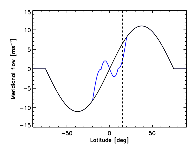
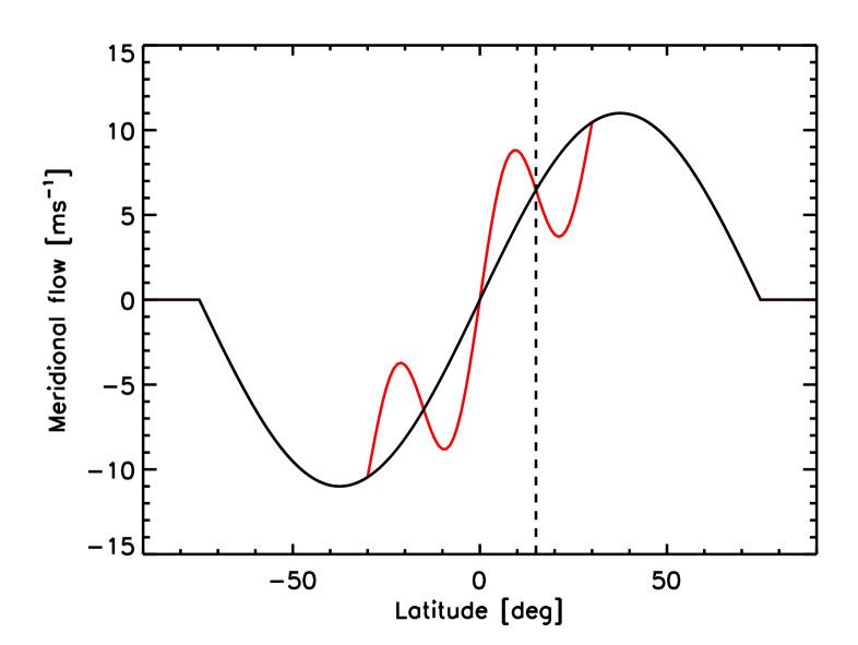
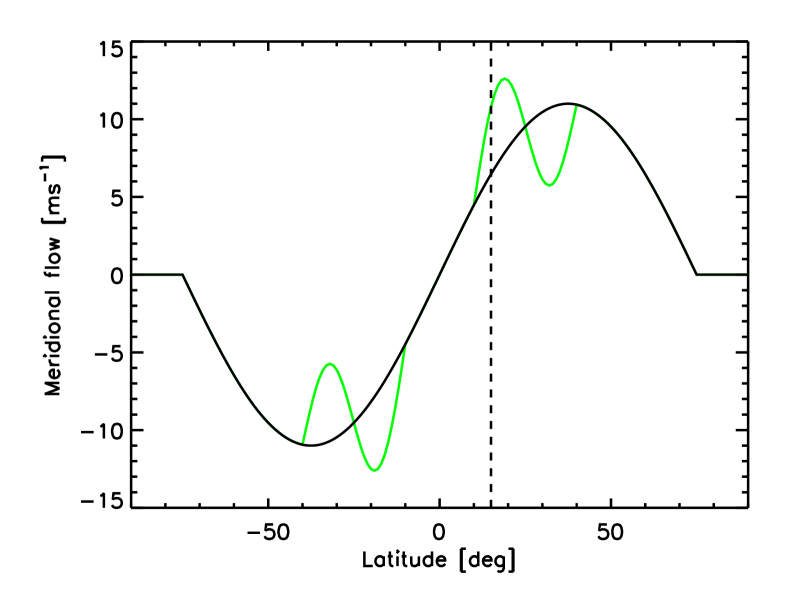
Figure 1: Meridional flow profiles considered for the simulations of a single bipole in a time-independent flow. Positive flow velocities are directed northward. The black curves in all panels show the profile without flow perturbation ($v_{0}=0$). The coloured curves represent the perturbed flow profiles for $v_{0}=5$ m s^-1, $\Delta\lambda_{v}=15^{\circ}$, and different central latitudes, $\lambda_{c}$, of the flow perturbation. Left panel: $\lambda_{c}=\pm 5^{\circ}$ (blue curve, coinciding with the black curve poleward of $\pm 20^{\circ}$); Middle panel: $\lambda_{c}=\pm 15^{\circ}$ (red curve, coinciding with the black curve poleward of $\pm 30^{\circ}$); Right panel: $\lambda_{c}=\pm 25^{\circ}$ (green curve, coinciding with the black curve poleward of $\pm 40^{\circ}$ and between $-10^{\circ}$ and $+10^{\circ}$). The dashed vertical lines indicate the mean latitude at which the bipolar region considered in Figure 2 is initiated.

In order to illustrate the effect of the meridional flow perturbation on the latitudinal flux transport as the source of the polar field, we first study a single bipolar magnetic region (BMR). The temporal evolution of the corresponding surface flux depends on the relative position of the bands of latitudinal flow perturbation and the emergence latitude. We consider the evolution of a BMR that emerges at $t=0$ at a latitude of $15^{\circ}$ on the northern hemisphere under the influence of four different meridional flow patterns (see Figure 1) described by Eqs. (2) and (6). The initial flux distribution of the BMR is chosen following the approach of Baumann et al. (2004).

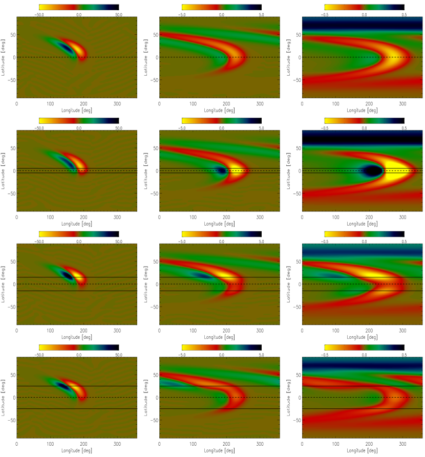
Figure 2: Evolution of the magnetic field distribution resulting from a single BMR with an initial unsigned flux of $1.9\,10^{23}$ Mx emerging at $t=0$ at a mean latitude of $15^{\circ}$ and with a tilt angle of $5.4^{\circ}$. Each row shows three snapshots (after 4, 12, and 24 Carrington rotations, respectively). The top row corresponds to the case without meridional flow perturbation ($v_{0}=0$, black curve in Figure 1). The rows below show the cases with perturbed flow ($v_{0}=5$ m s^-1, $\Delta\lambda_{v}=15^{\circ}$) centered at different latitudes: $\lambda_{c}=\pm 5^{\circ}$ (second row, blue curve in Figure 1), $\lambda_{c}=\pm 15^{\circ}$ (third row, red curve in Figure 1), and $\lambda_{c}=\pm 25^{\circ}$ (bottom row, green curve in Figure 1). The dashed lines indicate the equator while the full lines denote the central latitudes, $\pm\lambda_{c}$, of the flow perturbation. Magnetic field strengths are given in G. The full time evolution for these cases can be viewed with aid of the animations provided online as supplementary material.

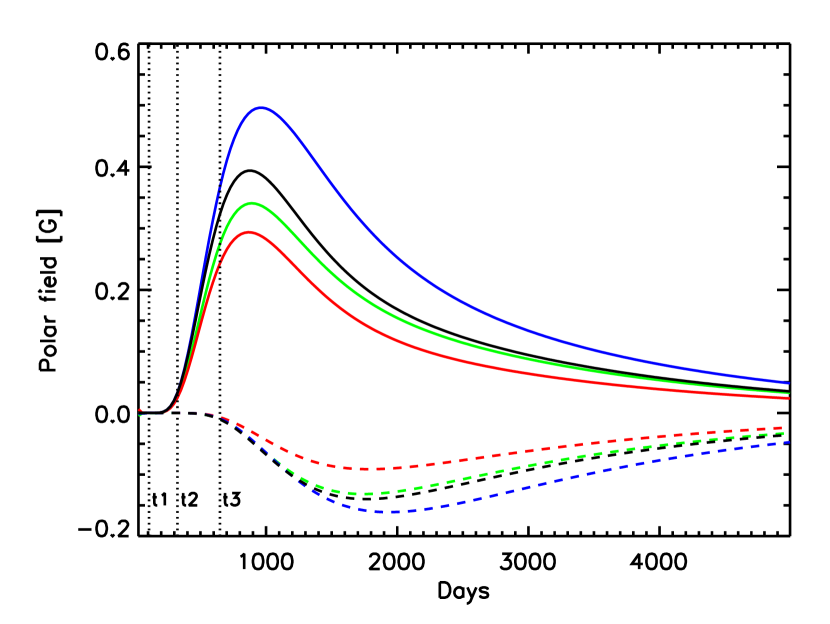
Figure 3: Temporal development of the polar cap field (average radial field poleward of $\pm 75^{\circ}$ latitude) for the simulations of single BMRs (solid lines: North, dashed lines: South) shown in Figure 2. The colors of the curves correspond to the four flow patterns given in Figure 1. The dotted vertical lines indicate the times ($t_{1},t_{2},t_{3}$) corresponding to the snapshots given in Figure 2.

Snapshots of the surface distribution of the magnetic field are shown in Figure 2. The four cases shown correspond to no flow perturbation (top row) and to converging flow bands centered on different latitudes $\lambda_{\rm c}$. The corresponding time evolution of the polar fields is shown in Figure 3. When the flow perturbation is centered equatorward of the BMR emergence latitude ($\lambda_{\rm c}=\pm 5^{\circ}$, second row in Figure 2), the overlap of the flow perturbations from both hemispheres (see blue curve in Figure 1) has the consequence that preceding and following polarities of the BMR experience an increased latitude separation: the leading polarity is advected toward the equator while the following polarity is less affected. As a consequence, the latitudinal separation between preceding and following polarity increases, so that the polar field becomes stronger in comparison to the case without flow perturbation. The opposite effect results in the case $\lambda_{\rm c}=\pm 15^{\circ}$ (third row in Figure 2, red curves in Figs. 1 and 3): now the latitudinal gradient of the meridional flow at the emergence location is such that the two polarities are now advected towards each other, thus reducing the azimuthally averaged field and, consequently, the flux reaching the pole. In the third case ($\lambda_{\rm c}=\pm 25^{\circ}$, fourth row in Figure 2, green curves in Figs. 1 and 3), there are two opposing effects: the meridional flow gradient near the emergence location tends to separate the polarities while the following polarity experiences an overall decrease of its poleward advection, thus tending to reduce the azimuthally averaged field. The net effect is a slight reduction of the contribution to the polar field.

These results show that the emergence location of a BMR relative to the position of the bands of flow perturbation is important for its effect on the development of the polar field. Note that the (axisymmetric) meridional flow perturbation considered here results from the cumulative effect of the individual inflows. A given active region (which can appear anywhere in the activity belt) therefore experiences the superposition of these inflows, which needs not necessarily be centered on this active region.

4 Simulation of activity cycles

4.1 Cycle parameters

As next step, we consider sequences of simulated activity cycles by periodically varying the number of BMRs that appear on the surface. The emerging BMRs have a tilt angle of half their emergence latitude, follow Hale’s polarity rules, and are introduced in activity belts that migrate toward the equator. The BMR area, $A$, follows the distribution $n(A)\propto A^{-2}$ derived from observations (Schrijver & Harvey, 1994). The number of BMRs emerging during the $i^{\rm th}$ cycle is taken to vary proportional to a Gaussian time profile, viz.

$$n_{i}(t) \propto \left\{\begin{array}[]{l l}\exp\{-[(t-t_{i}+6.5)/3.25]^{2}\}&0\leq(t-t_{i})\leq 13\\ 0&\mathrm{otherwise}\end{array}\right.$$ (9)

where $t_{i}=11\times i$ is the starting time of the $i^{\rm th}$ cycle and all times are in years. With new cycles starting every 11 years and having a duration of 13 years we thus take into account the overlap of solar activity cycles. The emergence of new BMRs occurs randomly with a Gaussian distribution of half-width $\Delta\lambda_{B}$ about the central latitudes of the activity belts, $\lambda_{\pm}$, which migrate equatorward according to

$$\lambda_{\pm}(t) = \pm[\lambda_{0}-(\lambda_{0}-8^{\circ})(t-t_{i})/13],$$ (10)

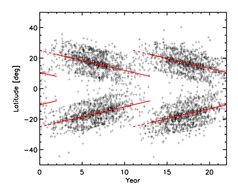
Figure 4: Time-latitude diagram of new BMRs (+ symbols) used as input for the flux transport simulation of solar cycles. The red lines indicate the central latitudes, $\lambda_{\pm}$, of the activity belts. The full parts of the red lines also give the centers of the bands of meridional flow perturbation (beginning 2 years after the start of the corresponding activity belt).

so that the belts progress from their starting latitudes, $\pm\lambda_{0}$, to $\pm 8^{\circ}$ in the course of 13 years. The resulting emergence pattern of new BMRs (butterfly diagram) for $\lambda_{0}=25^{\circ}$ and $\Delta\lambda_{B}=6^{\circ}$ is shown in Figure 4.

The latitudinal bands of the meridional flow perturbation move in parallel to the active region belts, their central latitudes (on both hemispheres), $\pm\lambda_{c}$, coinciding with the centers of the corresponding activity belts, $\lambda_{\pm}$. We do not assume an overlap of the meridional flow perturbations from consecutive cycles; therefore, we include the flow perturbation only for 11 years, starting from the third year of each 13-year cycle. Since the early flux emergence at mid latitudes affects the polar field only little, this assumption does not influence the results in a significant way (see also Section 4.4).

4.2 Dependence on the flow perturbation parameters

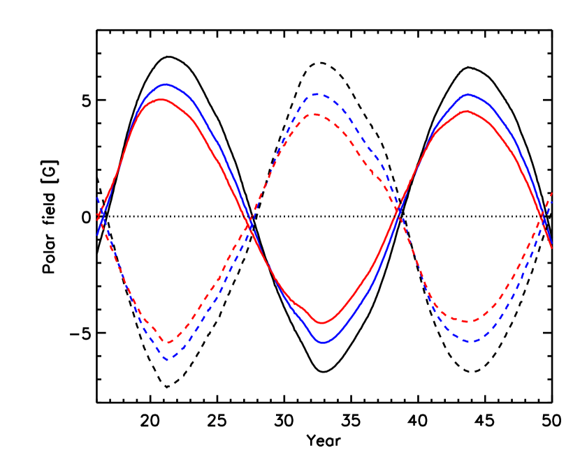
Figure 5: Time evolution of the polar field strength (average radial field poleward of $\pm 75^{\circ}$ latitude) for different values of the perturbation amplitude of the meridional flow: $v_{0}=0$ (black curve), $v_{0}=5$ m s^-1 (blue curve), $v_{0}=10$ m s^-1 (red curve). The width of the bands of perturbed flow was taken as $\Delta\lambda_{v}=15^{\circ}$.

Figure 5 shows the cyclic variation of the polar fields for three values of the flow perturbation amplitude: $v_{0}=(0,\,5,\,10)$ m s^-1. The latitudinal width of the bands was kept fixed at $\Delta\lambda_{v}=15^{\circ}$ and the activity belt parameters were $\lambda_{0}=25^{\circ}$ and $\Delta\lambda_{B}=6^{\circ}$. As already suggested by the results of the study of single BMRs shown in Section 3, we find that the net effect of the flow perturbation on BMRs emerging in an extended activity belt is a reduction of the polar field amplitudes. The effect becomes more pronounced with increasing flow perturbation amplitude.

On a more quantitative level, the dependence of the mean polar field amplitude (averages over three consecutive cycles) on the width, $\Delta\lambda_{v}$, and the amplitude, $v_{0}$, of the flow perturbation is given in Table 1. The numbers in parentheses give the percentage change of the polar field with respect to the case with unperturbed meridional flow. In all cases we find a reduction of the polar field. For parameters roughly corresponding to the helioseismic results $(v_{0}=5~{}$m s^-1, $\Delta\lambda_{v}=15^{\circ})$, the flow perturbation leads to a reduction of the polar field amplitude by about 18% with respect to the same case but without flow perturbation. Apart from the reduction becoming more pronounced with increasing perturbation amplitude, it also is stronger for bigger $\Delta\lambda_{v}$, i.e., for wider bands of perturbed flow. This is plausible because wider flow bands affect a larger proportion of the BMRs emerging in the activity belts and, at the same time, influence latitudinal flux advection for a longer time. In all cases, the evolution of the total unsigned surface flux is almost unaffected by the presence of the flow perturbation.

4.3 Dependence on the activity belt parameters

Keeping the parameters of the meridional flow perturbation fixed at values of $v_{0}=5$ m s^-1 and $\Delta\lambda_{v}=15^{\circ}$, we also considered the dependence of the polar field amplitude on the starting latitude, $\lambda_{0}$, and the width, $\Delta\lambda_{B}$, of the activity belt. The results are summarized in Table 2. As already suggested by the results of Section 3, the biggest effect on the polar field occurs when BMRs always emerge near the center (latitude of convergence) of the bands of perturbed flow, i.e., for $\Delta\lambda_{B}=0^{\circ}$. The flow perturbation then always tends to decrease the latitude extent of the BMR and thus reduces its azimuthally averaged field. The broader the activity belt (relative to the band of perturbed flow), the smaller is the effect on the polar field. On the other hand, for a given activity belt width, the variation of the starting latitude, $\lambda_{0}$, of the activity belt in a cycle does not significantly change the effect of the flow perturbation. In most cases, there is a tendency for the polar field amplitude to decrease with increasing $\lambda_{0}$. This result may have implications for the nonlinear limitation of a Babcock-Leighton dynamo as further discussed in Section 5.

4.4 Time-dependent flow perturbation amplitude

The observations based on helioseismology indicate that the amplitude of the axisymmetric flow perturbation peaks around the maximum of magnetic activity (González Hernández et al., 2010). We therefore also considered the effect of a temporal variation of the flow perturbation in parallel to the activity level. To this end, we modulated the perturbation amplitude, $v_{0}$, with the same time profile as that assumed for the number of emerging BMRs given by Equation (9), so that the maximum speed is reached at activity maximum. With the previously used parameters for the flow perturbation ($\upsilon_{0}=5\,\rm{m\,s^{-1}}$, $\Delta\lambda_{\upsilon}=15^{\circ}$) and for the width of the activity belt ($\Delta\lambda_{B}=6^{\circ}$), this results in a polar field with an amplitude (three-cycle average) of 5.66 G, about 2.5% higher than the value of 5.52 G found for constant flow perturbation amplitude. The effect of the time variation is somewhat stronger if we assume zero spread of the activity belt ($\Delta\lambda_{B}=0$); in this case we obtain a polar field of 5.22 G, which is about 6% higher than the corresponding value of 4.92 G for constant flow perturbation amplitude. This is to be expected since the polar field is dominated by the trans-equatorial transport (or cancellation) of leading-polarity flux; therefore, in the case of very narrow activity belts, the late phase of a cycle with flux emergence near the equator contributes more strongly to the strength of the polar field (Cameron & Schüssler, 2007).

Altogether, the effect of a temporal variation of the inflow amplitude is found to be rather small. Since the temporal modulation strongly reduces the flow perturbation during the rise and decay phases of a cycle, this result implies that the influence of the meridional flow perturbation on the polar field is dominated by the period around activity maximum.

5 Discussion and conclusion

The results presented here show that the observed cycle-related meridional flow perturbations in the form of bands migrating with the activity belts decrease the strength of the polar fields resulting from the latitudinal transport of surface flux. For a flow perturbation corresponding to the helioseismic observations, this reduction amounts to about 18% with respect to the case without flow perturbation. This indicates that these effects should be taken into account in surface flux transport simulations aiming at a quantitative pre- or postdiction of the polar field strength.

It is doubtful whether this kind of flow perturbation could have significantly contributed to the low polar polar field strength during the activity minimum between solar cycles 23 and 24 (e.g., Schrijver & Liu, 2008) as compared to previous minima: the perturbation is probably present during every cycle, so that only an increase of the perturbation in cycle 23 compared to its amplitude in previous cycles would contribute to a comparatively weaker polar field during the recent minimum. In any case, other effects must have been affecting the polar field in addition since the observed reduction by nearly a factor of 2 exceeds the decrease that could be caused by the flow perturbation considered here.

The observed variation of the flow perturbation amplitude during the activity cycle (González Hernández et al., 2010) and the probable contribution of the near-surface inflows toward active regions to the driving of the perturbations (Gizon & Rempel, 2008) suggest that the amplitude of the flow perturbation should increase with cycle strength. According to our results, this would lead to a stronger reduction of the polar field built up during cycles of higher activity. Since, in the framework of a Babcock-Leighton dynamo, the polar field is a measure of the poloidal field providing the basis for the toroidal field in the subsequent cycle, the meridional flow perturbation is potentially important for the nonlinear modulation and limitation of the cycle amplitude. Furthermore, we have also seen that the polar field decreases for increasing starting latitude, $\lambda_{0}$, of the activity belt at the beginning of a cycle. Since stronger cycles typically have higher values of $\lambda_{0}$ (Solanki et al., 2008), this relationship would strengthen the nonlinear effect of the flow perturbation in the subsequent cycle amplitude.

We conclude that, in addition to global variations of the meridional flow speed (Wang et al., 2002a, b), the cyclic perturbation of the meridional flow by converging bands migrating with activity belts has an appreciable effect on the build-up of the magnetic field at the polar caps. Its relation to the strength of a cycle means that the flow perturbation could be an important factor in determining the amplitude of Babcock-Leighton-type flux transport dynamos.

Table 1: Dependence of the polar field given in G on the parameters of the flow perturbation

	$\Delta\lambda_{\upsilon}$
		$10^{\circ}$		$15^{\circ}$		$20^{\circ}$
$\upsilon_{0}\rm{[m\,s^{-1}]}$
0.0		6.76		6.76		6.76
2.5		6.37 ($-6$%)		6.08 ($-10$%)		5.94 ($-12$%)
5.0		6.04 ($-10$%)		5.52 ($-18$%)		5.23 ($-23$%)
10.0		5.56 ($-18$%)		4.74 ($-30$%)		4.15 ($-39$%)

Table 2: Dependence of the polar field given in G on the activity belt parameters

		$\lambda_{0}=35^{\circ}$			$\lambda_{0}=25^{\circ}$			$\lambda_{0}=15^{\circ}$
$\upsilon_{0}\rm{[m\,s^{-1}]}$		0	5		0	5		0	5
$\Delta\lambda_{B}$
${\hskip-34.1433pt}0^{\circ}$		6.32	4.53 ($-28$%)		7.14	4.92 ($-31$%)		7.78	5.76 ($-25$%)
${\hskip-34.1433pt}6^{\circ}$		6.25	5.26 ($-15$%)		6.76	5.52 ($-18$%)		6.86	5.75 ($-16$%)
${\hskip-34.1433pt}12^{\circ}$		6.23	5.87 ($-6$%)		5.92	5.41 ($-8$%)		6.28	5.98 ($-5$%)

References

- Basu & Antia (2003) Basu, S. & Antia, H. M. 2003, ApJ, 585, 553
- Baumann et al. (2006) Baumann, I., Schmitt, D., & Schüssler, M. 2006, A&A, 446, 307
- Baumann et al. (2004) Baumann, I., Schmitt, D., Schüssler, M., & Solanki, S. K. 2004, A&A, 426, 1075
- Beck et al. (2002) Beck, J. G., Gizon, L., & Duvall, Jr., T. L. 2002, ApJ, 575, L47
- Cameron & Schüssler (2007) Cameron, R. & Schüssler, M. 2007, ApJ, 659, 801
- Chou & Dai (2001) Chou, D. & Dai, D. 2001, ApJ, 559, L175
- De Rosa & Schrijver (2006) De Rosa, M. L. & Schrijver, C. J. 2006, in ESA Special Publication, Vol. 624, Proceedings of SOHO 18/GONG 2006/HELAS I, Beyond the spherical Sun
- Dikpati et al. (2004) Dikpati, M., de Toma, G., Gilman, P. A., Arge, C. N., & White, O. R. 2004, ApJ, 601, 1136
- Gizon (2004) Gizon, L. 2004, Sol. Phys., 224, 217
- Gizon & Rempel (2008) Gizon, L. & Rempel, M. 2008, Sol. Phys., 251, 241
- González Hernández et al. (2010) González Hernández, I., Howe, R., Komm, R., & Hill, F. 2010, arXiv/astro-ph:1003.1685
- González Hernández et al. (2008) González Hernández, I., Kholikov, S., Hill, F., Howe, R., & Komm, R. 2008, Sol. Phys., 252, 235
- Haber et al. (2004) Haber, D. A., Hindman, B. W., Toomre, J., & Thompson, M. J. 2004, Sol. Phys., 220, 371
- Hathaway & Rightmire (2010) Hathaway, D. H. & Rightmire, L. 2010, Science, 327, 1350
- Hindman et al. (2004) Hindman, B. W., Gizon, L., Duvall, Jr., T. L., Haber, D. A., & Toomre, J. 2004, ApJ, 613, 1253
- Howard & Labonte (1980) Howard, R. & Labonte, B. J. 1980, ApJ, 239, L33
- Howe et al. (2006) Howe, R., Komm, R., Hill, F., Ulrich, R., Haber, D. A., Hindman, B. W., Schou, J., & Thompson, M. J. 2006, Sol. Phys., 235, 1
- Jiang et al. (2009) Jiang, J., Cameron, R., Schmitt, D., & Schüssler, M. 2009, ApJ, 693, L96
- Jiang et al. (2010) —. 2010, ApJ, 709, 301
- Komm (1994) Komm, R. W. 1994, Sol. Phys., 149, 417
- Komm et al. (1993) Komm, R. W., Howard, R. F., & Harvey, J. W. 1993, Sol. Phys., 147, 207
- Mackay et al. (2002) Mackay, D. H., Priest, E. R., & Lockwood, M. 2002, Sol. Phys., 209, 287
- Meunier (1999) Meunier, N. 1999, ApJ, 527, 967
- Ribes & Bonnefond (1990) Ribes, E. & Bonnefond, F. 1990, Geophysical and Astrophysical Fluid Dynamics, 55, 241
- Schrijver (2001) Schrijver, C. J. 2001, ApJ, 547, 475
- Schrijver & Harvey (1994) Schrijver, C. J. & Harvey, K. L. 1994, Sol. Phys., 150, 1
- Schrijver & Liu (2008) Schrijver, C. J. & Liu, Y. 2008, Sol. Phys., 252, 19
- Snodgrass (1983) Snodgrass, H. B. 1983, ApJ, 270, 288
- Solanki et al. (2008) Solanki, S. K., Wenzler, T., & Schmitt, D. 2008, A&A, 483, 623
- Wang et al. (2002a) Wang, Y., Lean, J., & Sheeley, Jr., N. R. 2002a, ApJ, 577, L53
- Wang et al. (2009) Wang, Y., Robbrecht, E., & Sheeley, N. R. 2009, ApJ, 707, 1372
- Wang et al. (2002b) Wang, Y., Sheeley, Jr., N. R., & Lean, J. 2002b, ApJ, 580, 1188
- Wang et al. (1989) Wang, Y.-M., Nash, A. G., & Sheeley, N. R. 1989, Science, 245, 712