Stochastic Exponential Integrators for a Finite Element Discretization of SPDEs

Abstract.

We consider the numerical approximation of general semilinear parabolic stochastic partial differential equations (SPDEs) driven by additive space-time noise. In contrast to the standard time stepping methods which uses basic increments of the noise and the approximation of the exponential function by a rational fraction, we introduce a new scheme, designed for finite elements, finite volumes or finite differences space discretization, similar to the schemes in [4, 7] for spectral methods and [1] for finite element methods. We use the projection operator, the smoothing effect of the positive definite self-adjoint operator and linear functionals of the noise in Fourier space to obtain higher order approximations. We consider noise that is white in time and either in $H^{1}$ or $H^{2}$ in space and give convergence proofs in the mean square $L^{2}$ norm for a diffusion reaction equation and in mean square $H^{1}$ norm in the presence of an advection term. For the exponential integrator we rely on computing the exponential of a non-diagonal matrix. In our numerical results we use two different efficient techniques: the real fast Léja points and Krylov subspace techniques. We present results for a linear reaction diffusion equation in two dimensions as well as a nonlinear example of two-dimensional stochastic advection diffusion reaction equation motivated from realistic porous media flow.

1. Introduction

We consider the strong numerical approximation of Ito stochastic partial differential equations

(1.1) $$dX=(AX+F(X,\nabla X))dt+dW$$

in a Hilbert space $H=L^{2}(\Omega)$, where $\Omega\subset\mathbb{R}^{d}$ and $t\in[0,T]$, $T>0$ and initial data $X(0)=X_{0}$ is given. The linear operator $A$ is the generator of an analytic semigroup $S(t):=e^{tA},t\geq 0\;$ with eigenfunctions $e_{i},\;i\in\mathbb{N}^{d}$ and $F$ is a nonlinear function. The noise can be represented as a series in the eigenfunctions of the covariance operator $Q$ and we assume for convenience that $Q$ and $A$ have the same eigenfunctions (without loss the generality as the orthogonal projection can be used). In which case [24] we have

(1.2) $$W(x,t)=\underset{i\in\mathbb{N}^{d}}{\sum}\sqrt{q_{i}}e_{i}(x)\beta_{i}(t),$$

where $q_{i}$, $i\in\mathbb{N}^{d}$ are the eigenvalues of the covariance operator $Q$. The $\beta_{i}$ are independent and identically distributed standard Brownian motions.

The study of numerical solutions of SPDEs is an active research area and there is an extensive literature on numerical methods for SPDEs. Recent work by Jentzen and co-workers [2, 3, 4, 7] uses the Taylor expansion and linear functionals of the noise for Fourier–Galerkin discretizations of (1.1). In these schemes the diagonalization of the operator $A$ through the discretization plays a key role. Using a linear functional of the noise overcomes the order barrier encountered using a standard increment of Wiener process [4]. In [1] the use of linear functionals of the noise is extended to finite–element discretizations (where the operator does not diagonalize) with a semi-implicit Euler–Maruyama method. In contrast to [1] here we consider two exponential based methods for time-stepping as in [21, 20, 4, 7, 19]. We prove a strong convergence result for two versions of the scheme with noise that is white in time and in $H^{1}$ and $H^{2}$ in space that shows that the exponential integrators are more accurate that the semi-implicit Euler-Maruyama method. Furthermore we have weaker restrictions on the regularity of the initial data and high accuracy for linear problems comparing to the scheme in [1]. The cost of the extra accuracy though is that to implement these methods we need to compute the exponential of a non–diagonal matrix, which is a notorious problem in numerical analysis [35]. However, new developments for both Léja points and Krylov subspace techniques [33, 34, 17, 39, 31, 32] have led to efficient methods for computing matrix exponentials. Compared to the Fourier-Galerkin methods of [2, 3, 4, 7] we gain the flexibility of finite element (or finite volume methods) to deal with complex boundary conditions and we can apply well developed techniques such as upwinding to deal with advection.

We consider two examples of (1.1) where $A$ is the second order operator $D\varDelta$ and $D>0$ is the diffusion coefficient. For the first example

(1.3) $$dX=\left(D\varDelta X-\lambda X\right)dt+dW$$

where $\lambda$ is a constant, we can construct an exact solution. Our second example is a stochastic advection diffusion reaction equation in a heterogeneous porous media

(1.4) $$dX=\left(D\varDelta X-\nabla\cdot(\textbf{q}X)-\frac{X}{X+1}\right)dt+dW$$

where q is the Darcy velocity field [22]. In the linear example we take Neumann boundary conditions and for the example from porous media we take a mixed Neumann–Dirichlet boundary condition.

The paper is organised as follows. In Section 2 we present the two numerical schemes based on the exponential integrators and our assumptions on (1.1). We present and comment on our convergence results. In Section 3 we present the proofs of our convergence theorems. We conclude in Section 4 by presenting some simulations and discuss implementation of these methods.

2. Numerical scheme and main results

We start by introducing our notation. We denote by $\|\cdot\|$ the norm associated to the standard inner product $(\cdot,\cdot)$ of the Hilbert space $H=L^{2}(\Omega)$ and $\|\cdot\|_{H^{m}(\Omega)}$ the norm of the Sobolev space $H^{m}(\Omega)$, for $m\in\mathbb{R}$. For a Banach space $\mathcal{V}$ we denote by $L(\mathcal{V})$ the set of bounded linear mapping from $\mathcal{V}$ to $\mathcal{V}$ and $L^{(2)}(\mathcal{V})$ the set of bounded bilinear mapping from $\mathcal{V}\times\mathcal{V}$ to $\mathbb{C}$. We introduce further spaces and notation below as required.

Consider the stochastic partial differential equation (1.1), under some technical assumptions it is well known (see [24, 23, 2] and references therein) that the unique mild solution is given by

(2.1) $$X(t) = S(t)X_{0}+\int_{0}^{t}S(t-s)F(X(s))ds+O(t),$$

with the stochastic process $O$ given by the stochastic convolution

(2.2) $$O(t)=\int_{0}^{t}S(t-s)dW(s).$$

We consider discretization of the spatial domain by a finite element triangulation. Let $\mathcal{T}_{h}$ be a set of disjoint intervals of $\Omega$ (for $d=1$), a triangulation of $\Omega$ (for $d=2$) or a set of tetrahedra (for $d=3$). Let $V_{h}$ denote the space of continuous functions that are piecewise linear over $\mathcal{T}_{h}$. To discretize in space we introduce two projections. Our first projection operator $P_{h}$ is the $L^{2}(\Omega)$ projection onto $V_{h}$ defined for $u\in L^{2}(\Omega)$ by

(2.3) $$(P_{h}u,\chi)=(u,\chi)\qquad\forall\;\chi\in V_{h}.$$

We can then define the operator $A_{h}:V_{h}\rightarrow V_{h}$, the discrete analogue of $A$, by

(2.4) $$(A_{h}\varphi,\chi)=(A\varphi,\chi)\qquad\varphi,\chi\in V_{h}.$$

We denote by $S_{h}(t):=e^{tA_{h}}$ the semigroup generated by the operator $A_{h}$. The second projection $P_{N}$, $N\in\mathbb{N}$ is the projection onto a finite number of spectral modes ${e_{i}}$ defined for $u\in L^{2}(\Omega)$ by

$$u^{N}:=P_{N}u=\sum_{i=1}^{N}(e_{i},u)e_{i}.$$

Furthermore we can project the operator $A$

$$A_{N}=P_{N}A\quad\text{and}\quad S_{N}(t):=e^{tA_{N}}.$$

We discretize in space using finite elements and project the noise first onto a finite number of modes and then onto the finite element space. The semi-discretized version of (1.1) is to find the process $X^{h}(t)=X^{h}(.,t)\in V_{h}$ such that

(2.5) $$dX^{h}=(A_{h}X^{h}+P_{h}F(X^{h}))dt+P_{h}P_{N}dW,\quad X^{h}(0)=P_{h}X_{0}.$$

The mild solution of (2.5) at time $t_{m}=m\Delta t$, $\Delta t>0$ is given by

$$X^{h}(t_{m})=S_{h}(t_{m})P_{h}X_{0}+\int_{0}^{t_{m}}S_{h}(t_{m}-s)P_{h}F(X^{h}(s))ds+\int_{0}^{t_{m}}S_{h}(t_{m}-s)P_{h}dW^{N}(s).$$

Given the mild solution at the time $t_{m}$, we can construct the corresponding solution at $t_{m+1}$ as

(2.6) $$X^{h}(t_{m+1}) = S_{h}(\Delta t)X^{h}(t_{m})+\int_{0}^{\Delta t}S_{h}(\Delta t-s)P_{h}F(X^{h}(s+t_{m}))ds$$

$$+\int_{t_{m}}^{t_{m+1}}S_{h}(t_{m+1}-s)P_{h}dW^{N}(s).$$

For our first numerical scheme (SETD1), we use the following approximations

$$F(X^{h}(t_{m}+s)) \approx F(X^{h}(t_{m}))\qquad s\in[0,\;\Delta t],$$

and

$$\int_{t_{m}}^{t_{m+1}}S_{h}(t_{m+1}-s)P_{h}dW^{N}(s) \approx P_{h}\int_{t_{m}}^{t_{m+1}}S_{N}(t_{m+1}-s)dW^{N}(s)$$

$$= P_{h}P_{N}\int_{t_{m}}^{t_{m+1}}S(t_{m+1}-s)dW(s).$$

Then we approximate $X_{m}^{h}$ of $X(m\Delta t)$ by

$$X_{m+1}^{h} = e^{\Delta tA_{h}}X_{m}^{h}+\Delta t\varphi_{1}(\Delta tA_{h})P_{h}F(X_{m}^{h})$$

$$+ P_{h}\int_{t_{m}}^{t_{m+1}}e^{(t_{m+1}-s)A_{N}}dW^{N}(s)$$

where

$$\varphi_{1}(\Delta tA_{h})=(\Delta t\,A_{h})^{-1}\left(e^{\Delta tA_{h}}-I\right)=\frac{1}{\Delta t}\int_{0}^{\Delta t}e^{(\Delta t-s)A_{h}}ds.$$

For efficiency to avoid computing two matrix exponentials we can rewrite the scheme (2) as

$$X_{m+1}^{h}=X_{m}^{h}+\Delta t\varphi_{1}(\Delta tA_{h})\left(A_{h}X_{m}^{h}\\ +P_{h}F(X_{m}^{h})\right)+P_{h}\int_{t_{m}}^{t_{m+1}}e^{(t_{m+1}-s)A_{N}}dW^{N}(s).$$

We call this scheme (SETD1).

Our second numerical method (SETD0) is similar to the one in [21, 20, 19]. It is based on approximating the deterministic integral in (2.6) at the left–hand endpoint of each partition and the stochastic integral as follows

$$\int_{t_{m}}^{t_{m+1}}S_{h}(t_{m+1}-s)P_{h}dW^{N}(s) \approx P_{h}\int_{t_{m}}^{t_{m+1}}S_{N}(t_{m+1}-s)dW^{N}(s)$$

$$= P_{h}P_{N}\int_{t_{m}}^{t_{m+1}}S(t_{m+1}-s)dW(s).$$

With this we can define the (SETD0) approximation $Y_{m}^{h}$ of $X(m\Delta t)$ by

(2.8) $$\qquad Y_{m+1}^{h}=\varphi_{0}(\Delta tA_{h})\left(Y_{m}^{h}+\Delta tP_{h}F(Y_{m}^{h})\right)+P_{h}\int_{t_{m}}^{t_{m+1}}e^{(t_{m+1}-s)A_{N}}dW^{N}(s)$$

where

$$\varphi_{0}(\Delta tA_{h})=e^{\Delta tA_{h}}.$$

If we project the eigenfunctions of $Q$ onto the eigenfunctions of the linear operator $A$ then by a Fourier spectral method the process

$$\widehat{O}_{k}=\int_{t_{k}}^{t_{k+1}}e^{(t_{k+1}-s)A_{N}}dW^{N}(s)$$

is reduced to an Ornstein–Uhlenbeck process in each Fourier mode as in [4] and we therefore know the exact variance in each mode. We comment further on the implementation in Section 4. We describe now in detail the assumptions that we make on the linear operator $A$, on our finite element discretization, the nonlinear term $F$ and the noise $dW$.

Assumption 1.

Let the linear operator $-A$ be a self adjoint positive definite operator and $A$ generate an analytic semigroup $S$. Then there exist sequences of positive real eigenvalues $\{\lambda_{n}\}_{n\in\mathbb{N}^{d}}$ and an orthonormal basis in $H$ of eigenfunctions $\{e_{i}\}_{i\in\mathbb{N}^{d}}$ such that the linear operator $-A:\mathcal{D}(-A)\subset H\rightarrow H$ is represented as

$$-Av=\underset{i\in\mathbb{N}^{d}}{\sum}\lambda_{i}(e_{i},v)e_{i}\qquad\forall\quad v\in\mathcal{D}(-A)$$

where the domain of $-A$, $\mathcal{D}(-A)=\{v\in H:\underset{i\in\mathbb{N}^{d}}{\sum}\lambda_{i}^{2}|(e_{i},v)|<\infty\}$ and $\underset{i\in\mathbb{N}^{d}}{\inf}\lambda_{i}>0$ .

Note that for convenience of presentation we take $A$ to be a second order operator as this simplifies notation for the norm equivalence below. Similar result hold, however, for higher order operators. We recall some basic properties of the semigroup $S(t)$ generated by $A$ that may be found for example in [13, 25].

Proposition 2.1 ([13]).

Let $\beta\geq 0$ and $0\leq\gamma\leq 1$, then there exist $C>0$ such that

$$\|(-A)^{\beta}S(t)\| \leq Ct^{-\beta}\;\;\;\;\;\text{for }\;\;\;t>0$$

$$\|(-A)^{-\gamma}(\text{I}-S(t))\| \leq Ct^{\gamma}\;\;\;\;\;\text{for }\;\;\;t\geq 0.$$

In addition,

$$(-A)^{\beta}S(t) = S(t)(-A)^{\beta}\quad\text{on}\quad\mathcal{D}((-A)^{\beta})$$

$$\text{If}\;\;\;\beta \geq \gamma\quad\text{then}\quad\mathcal{D}((-A)^{\beta})\subset\mathcal{D}((-A)^{\gamma}).$$

We introduce two spaces $\mathbb{H}$ and $V$ where $\mathbb{H}\subset V$ that depend on the choice of the boundary conditions. For Dirichlet boundary conditions we let

$$V=\mathbb{H}=H_{0}^{1}(\Omega)=\{v\in H^{1}(\Omega):v=0\;\;\text{on}\;\;\partial\Omega\},$$

and for Robin boundary conditions, for which Neumann boundary conditions are a particular case, $V=H^{1}(\Omega)$ and

$$\mathbb{H}=\left\{v\in H^{1}(\Omega):\partial v/\partial\nu_{A}+\sigma v=0\quad\text{on}\quad\partial\Omega\right\},$$

see [16] for details. Functions in $\mathbb{H}$ satisfy the boundary conditions and with $\mathbb{H}$ in hand we can characterize the domain of the operator $(-A)^{r/2}$ and have the following norm equivalence [14, 26] for $r=1,2$

$$\|v\|_{H^{r}(\Omega)}\equiv\|(-A)^{r/2}v\|_{L^{2}(\Omega)}:=\|v\|_{r},\qquad\forall v\in\mathcal{D}((-A)^{r/2})=\mathbb{H}\cap H^{r}(\Omega).$$

We now introduce our assumptions on the spatial domain and finite element space $V_{h}$. We consider the space of continuous functions that are piecewise linear over the triangulation $\mathcal{T}_{h}$ with $V_{h}\subset V$.

Assumption 2.

(Regularity of the domain $\Omega$ and the space grid)

We assume that $\Omega$ has a smooth boundary or is a convex polygon and that the maximal length $h$ of the elements of $\mathcal{T}_{h}$ satisfy the usual regularity assumptions on the triangulation i.e. for $r=1,2$

(2.9) $$\underset{\chi\in V_{h}}{\inf}\left(\|v-\chi\|+h\|\nabla(v-\chi)\|\right)\leq Ch^{r}\|v\|_{H^{r}(\Omega)},\qquad v\in V\cap H^{r}(\Omega).$$

This inequality is sometimes called the Bramble and Hilbert inequality, see [16] or [15]. It follows that

(2.10) $$\|P_{h}v-v\|\leq Ch^{r}\|v\|_{H^{r}(\Omega)}\qquad\forall v\in V\cap H^{r}(\Omega),\quad r=1,2.$$

Assumption 3.

(Nonlinearity)

Let $\mathcal{V}$ be a separable Banach space such that $\mathcal{D}((-A)^{1/2})\subset\mathcal{V}\subset H=L^{2}(\Omega)$ continuously. We assume that there exist a positive constant $L>0$ such that the Nemytskii operator $F$ satisfies one of the following

(a) $F:\mathcal{V}\rightarrow\mathcal{V}$ is twice continuously Fréchet differentiable mapping with

$$\|F^{\prime}(v)w\|\leq L\|w\|,\qquad\|F^{\prime}(v)\|_{L(\mathcal{V})}\leq L,\qquad\|F^{\prime\prime}(v)\|_{L^{(2)}(\mathcal{V})}\leq L$$

and

$$\|(F^{\prime}(u))^{*}\|_{L(\mathcal{D}((-A)^{1/2}))}\leq L(1+\|u\|_{\mathcal{D}((-A)^{1/2})})\qquad\forall\,v,w\in\mathcal{V},\quad u\in\mathcal{D}((-A)^{1/2}),$$

where $(F^{\prime}(u))^{*}$ is the adjoint of $F^{\prime}(u)$ defined by

$$((F^{\prime}(u))^{*}v,w)=(v,F^{\prime}(u)w)\;\;\ \forall\,v,w\in H=L^{2}(\Omega).$$

As a consequence

$$\|F(X)-F(Y)\|\leq L\|X-Y\|\qquad\forall X,Y\in H,$$

and $\forall X\in H=L^{2}(\Omega)$

$$\|F(X)\|\leq\|F(0)\|+\|F(X)-F(0)\|\leq\|F(0)\|+L\|X\|\leq C(\|F(0)\|+\|X\|).$$

(b) $F$ is globally Lipschitz continuous from $(H^{1}(\Omega),\|.\|_{H^{1}(\Omega)})$ to $(H=L^{2}(\Omega),\|.\|)$ then

$$\|F(X)-F(Y)\|\leq L\|X-Y\|_{H^{1}(\Omega)}\qquad\forall X,Y\in H^{1}(\Omega).$$

We assume that the function $F$ is defined in $L^{2}(\Omega)$, although in general $F$ may be defined in any Hilbert space. The possible choice of $\mathcal{V}$ can be $H$, $H^{1}(\Omega)$ or the $\mathbb{R}-$ Banach space of continuous functions from $[0,T]$ to $H$ denoted by $C([0,T],H)$ if $d=1$.

We now turn our attention to the noise term and introduce spaces and notation that we need to define the $Q$-Wiener process. Denoting by $\mathcal{L}(H)$ the Banach algebra of bounded linear operators on $H$ with the usual norm. We recall that an operator $T\in\mathcal{L}(H)$ is Hilbert-Schmidt if

$$\|T\|_{HS}^{2}:=\underset{i\in\mathbb{N}^{d}}{\sum}\|Te_{i}\|^{2}<\infty.$$

If we denote the space of Hilbert-Schmidt operator from $Q^{1/2}(H)$ to $H$ by $L_{2}^{0}:=HS(Q^{1/2}(H),H)$ i.e

$$L_{2}^{0}=\left\{\varphi\in\mathcal{L}(H):\underset{i\in\mathbb{N}^{d}}{\sum}\|\varphi\,Q^{1/2}e_{i}\|^{2}<\infty\right\},$$

the corresponding norm $\|.\|_{L_{2}^{0}}$ by

$$\|\varphi\,\|_{L_{2}^{0}}:=\|\varphi Q^{1/2}\|_{HS}=\left(\underset{i\in\mathbb{N}^{d}}{\sum}\|\varphi Q^{1/2}e_{i}\|^{2}\right)^{1/2}.$$

Let $\varphi(\omega)$ be a process such that for every sample $\omega$, $\varphi(\omega)\in L_{2}^{0}$. Then we have the following equality

$$\textbf{E}\|\int_{0}^{t}\varphi dW\|^{2}=\int_{0}^{t}\textbf{E}\|\varphi\|_{L_{2}^{0}}^{2}ds=\int_{0}^{t}\textbf{E}\|\varphi Q^{1/2}\|_{HS}ds,$$

using Ito’s isometry [24]. We assume sufficient regularity of the noise for the existence of a mild solution and to project the noise into the finite element space $V_{h}$. To be specific we assume the noise is in either in $H^{1}$ or $H^{2}$ in space.

Assumption 4.

(Regularity of the noise) For all $t\in[0,T]$ we assume that $O(t)$ is an adapted stochastic process to the filtration $(\mathcal{F}_{t})_{t\geq 0}$ with continuous sample paths such that $O(t_{2})-S(t_{2}-t_{1})O(t_{1}),\;0\leq t_{1}<t_{2}\leq T$ is independent of $\mathcal{F}_{t_{1}}$ Let $\mathcal{V}$ be a separable Banach space such that $\mathcal{D}((-A)^{1/2})\subset\mathcal{V}\subset H=L^{2}(\Omega)$ continuously. For some $\theta\in(0,1/2]$

$$O(t)\in\mathcal{D}((-A)^{r/2}) = \mathbb{H}\cap H^{r}(\Omega),\qquad r=1,2$$

$$\textbf{E}\left(\|O(t_{2})-O(t_{1})\|_{\mathcal{V}}^{4}\right) \leq C(t_{2}-t_{1})^{4\theta}.$$

Using the equivalence of norms, we have that

$$O(t)\in\mathcal{D}((-A)^{r/2})\quad\forall t\in[0,T]\Leftrightarrow\|(-A)^{r/2}Q^{1/2}\|_{HS}<\infty\quad r=1,2.$$

2.1. Main results

Throughout the paper we let $N$ be the number of terms of truncated noise and $\mathcal{I}_{N}=\left\{1,2,...,N\right\}^{d}$ and take $t_{m}=m\Delta t\in(0,T]$, where $T=M\Delta t$ for $m,M\in\mathbb{N}$. We take $C$ to be a constant that may depend on $T$ and other parameters but not on $\Delta t$, $N$ or $h$. We also assume that when initial data $X_{0}\in\mathcal{D}((-A)^{\gamma})$ then $\mathbf{E}\|(-A)^{\gamma}X_{0}\|^{l}<\infty$, $l=2,4$ and $0\leq\gamma<1$.

Our first result is a strong convergence result in $L^{2}$ when the non-linearity satisfies the Lipschitz condition of Assumption 3 (a) with scheme (SETD1). This is, for example, the case of reaction–diffusion SPDEs.

Theorem 2.2.

Suppose that Assumptions 1, 2, 3(a) and 4 are satisfied with $r=1,2$. Let $X(t_{m})$ be the mild solution of equation (1.1) represented by (2.1) and $X_{m}^{h}$ be the numerical approximation through (2) (SETD1). Let $0<\gamma<1$ and set $\sigma=\min(2\theta,\gamma)$ and let $\theta\in(0,1/2]$ be defined as in Assumption 4.

If $X_{0}\in\mathcal{D}((-A)^{\gamma})$ then

$$\left(\textbf{E}\|X(t_{m})-X_{m}^{h}\|^{2}\right)^{1/2} \leq C\left(t_{m}^{-1/2}h^{r}+\Delta t^{\sigma}+\left(\underset{j\in\mathbb{N}^{d}\backslash\mathcal{I}_{N}}{\inf}\lambda_{j}\right)^{-r/2}\right).$$

If $X_{0}\in\mathcal{D}(-A)=\mathbb{H}\cap H^{2}(\Omega)$ then

$$\left(\textbf{E}\|X(t_{m})-X_{m}^{h}\|^{2}\right)^{1/2}\leq C\left(h^{r}+\Delta t^{2\theta}+\left(\underset{j\in\mathbb{N}^{d}\backslash\mathcal{I}_{N}}{\inf}\lambda_{j}\right)^{-r/2}\right).$$

Our first result for scheme (SETD0) is a strong convergence result in $L^{2}$ when the non-linearity satisfies the Lipschitz condition of Assumption 3 (a).

Theorem 2.3.

Suppose that Assumptions 1, 2, 3(a) and 4 are satisfied with $r=1,2$. Let $X(t_{m})$ be the mild solution of equation (1.1) represented by (2.1) and $Y_{m}^{h}$ be the numerical approximation through (2.8) (SETD0). Let $0<\gamma<1$ and set $\sigma=\min(2\theta,\gamma)$ and let $\theta\in(0,1/2]$ be defined as in Assumption 4.

If $X_{0}\in\mathcal{D}((-A)^{\gamma})$ then

$$\left(\textbf{E}\|X(t_{m})-Y_{m}^{h}\|^{2}\right)^{1/2} \leq C\left(t_{m}^{-1/2}h^{r}+\Delta t^{\sigma}+\Delta t\left|\ln(\Delta t)\right|+\left(\underset{j\in\mathbb{N}^{d}\backslash\mathcal{I}_{N}}{\inf}\lambda_{j}\right)^{-r/2}\right).$$

If $X_{0}\in\mathcal{D}(-A)=\mathbb{H}\cap H^{2}(\Omega)$ then

$$\left(\textbf{E}\|X(t_{m})-Y_{m}^{h}\|^{2}\right)^{1/2}\leq C\left(h^{r}+\Delta t^{2\theta}+\Delta t\left|\ln(\Delta t)\right|+\left(\underset{j\in\mathbb{N}^{d}\backslash\mathcal{I}_{N}}{\inf}\lambda_{j}\right)^{-r/2}\right).$$

For convergence in the mean square $H^{1}(\Omega)$ norm where the non-linearity satisfies the Lipschitz condition from $L^{2}(\Omega)$ norm to $H^{1}(\Omega)$ ( Assumption 3 (b)) we can state results for (SETD1) and (SETD0) together.

Theorem 2.4.

Suppose that Assumptions 1, 2, 3(b), 4 (with $r=2$) are satisfied and $F(X)\in V$ with $\mathbf{E}\left(\underset{0\leq s\leq T}{\sup}\|F(X(s))\|_{H^{1}(\Omega)}\right)^{2}<\infty$. Let $X$ be the solution mild of equation (1.1) represented by equation (2.1) and $\zeta_{m}^{h}$ be the numerical approximations through scheme (2) or (2.8) ( $\zeta_{m}^{h}=X_{m}^{h}$ for scheme (SETD1) and $\zeta_{m}^{h}=Y_{m}^{h}$ for scheme (SETD0)). Let $0\leq\gamma<1$. Then we have the following:

If $X_{0}\in\mathcal{D}((-A)^{(1+\gamma)/2})$ then

$$(\textbf{E}\|X(t_{m})-\zeta_{m}^{h}\|_{H^{1}(\Omega)}^{2})^{1/2} \leq C\left((t_{m}^{-1/2}\,h+\Delta t^{\gamma/2})+\left(\underset{j\in\mathbb{N}^{d}\backslash\mathcal{I}_{N}}{\inf}\lambda_{j}\right)^{-1/2}\right).$$

If $X_{0}\in\mathcal{D}((-A))$ then

$$(\textbf{E}\|X(t_{m})-\zeta_{m}^{h}\|_{H^{1}(\Omega)}^{2})^{1/2} \leq C\left((h+\Delta t^{1/2-\epsilon})+\left(\underset{j\in\mathbb{N}^{d}\backslash\mathcal{I}_{N}}{\inf}\lambda_{j}\right)^{-1/2}\right).$$

for very small $\epsilon\in(0,1/2)$.

We note that this theorem covers the case of advection-diffusion-reaction SPDEs, such as that arising in our example from porous media.

We remark that if we denote by $N_{h}$ the numbers of vertices in the finite elements mesh then it is well known (see for example [27]) that if $N\geq N_{h}\$ then

$$\left(\underset{j\in\mathbb{N}^{d}\backslash\mathcal{I}_{N}}{\inf}\lambda_{j}\right)^{-1}\leq Ch^{2}\qquad\text{and}\qquad\left(\underset{j\in\mathbb{N}^{d}\backslash\mathcal{I}_{N}}{\inf}\lambda_{j}\right)^{-1/2}\leq Ch.$$

As a consequence the estimates in Theorem 2.2, Theorem 2.3 and Theorem 2.4 can be expressed in function of $h$ and $\Delta t$ only and it is the error from the finite element approximation that dominates. If $N\leq N_{h}$ then it is the error from the projection $P_{N}$ of the noise onto a finite number of modes that dominates.

From Theorem 2.4 we also get an estimate in the root mean square $L^{2}(\Omega)$ norm in the case that the nonlinear function $F$ satisfies Assumption 3 (b). We cannot do the proof directly in $L^{2}(\Omega)$ due to the Lipschitz condition in Assumption 3 (b). Simulations for Theorem 2.4 will be do in $L^{2}(\Omega)$ since the discrete $L^{2}(\Omega)$ norm is more easy to use in all type of boundary conditions.

Finally if we compare these theorems to those in [1] for a modified semi-implicit Euler-Maruyama method then we see that using the exponential based integrators we have weaker conditions on the initial data and in particular the scheme (SETD1) has better convergence properties.

3. Proofs of main results

3.1. Preparatory results

We start by examining the deterministic linear problem. Find $u\in V$ such that such that

(3.1) $$u^{\prime}=Au\qquad\text{given}\quad u(0)=v.$$

The corresponding semi-discretization in space is : find $u_{h}\in V_{h}$ such that

$$u_{h}^{\prime}=A_{h}u_{h}$$

where $u_{h}^{0}=P_{h}v$. Define the operator

(3.2) $$T_{h}(t):=S(t)-S_{h}(t)P_{h}=e^{tA}-e^{tA_{h}}P_{h}$$

so that $u(t)-u_{h}(t)=T_{h}(t)v$.

Lemma 3.1.

The following estimates hold on the semi-discrete approximation of (3.1)

(3.3) $$\|u(t)-u_{h}(t)\| = \|T_{h}(t)v\|\leq Ct^{-1/2}\;h^{2}\|v\|\;\;\;\;\;\text{if}\;\;\;v\in H=L^{2}(\Omega),$$

(3.4) $$\|u(t)-u_{h}(t)\| = \|T_{h}(t)v\|\leq Ch^{2}\|v\|_{H^{2}(\Omega)}\;\;\;\text{if}\;\;\;v\in\mathcal{D}((-A)),$$

(3.5) $$\|u(t)-u_{h}(t)\|_{H^{1}(\Omega)} = \|T_{h}(t)v\|_{H^{1}(\Omega)}\leq Cht^{-1/2}\|v\|_{H^{1}(\Omega)}\;\;\;\text{if}\;\;\;v\in V,$$

(3.6) $$\|u(t)-u_{h}(t)\|_{H^{1}(\Omega)} = \|T_{h}(t)v\|_{H^{1}(\Omega)}\leq Ch\|v\|_{H^{2}(\Omega)}\;\;\;\text{if}\;\;\;v\in\mathcal{D}(-A).$$

Proof.

The proof of the estimates (3.3) and (3.4) can be found in [15] with Dirichlet boundary conditions. The same proof can be generalized easily to Robin or mixed boundary conditions, incorporating the extra term from the boundary with the bilinear form. Estimates (3.3)- (3.6) are the special case of the proof of Theorem 3.1 in [14] where the nonlinearity is taken to be zero. For our case

$$u(t)=S(t)v,$$

and we have the following estimates for $t\in(0,T]$

$$\|u(t)\|_{H^{s}(\Omega)} \leq Ct^{-(s-1)/2}\|v\|_{H^{1}(\Omega)}\;\;\;\;\;\text{if}\;\;\;v\in\mathbb{H}\;\;\;\;\;s=1,2,$$

$$\|u(t)\|_{H^{2}(\Omega)} \leq C\|v\|_{H^{2}(\Omega)}\;\;\;\;\;\text{if}\;\;\;v\in\mathcal{D}(-A),$$

$$\|u_{t}(t)\|_{H^{s}(\Omega)} \leq Ct^{-1-(s-1)/2}\|v\|_{H^{1}(\Omega)}\;\;\;\;\;\text{if}\;\;\;v\in\mathbb{H}\;\;\;s=0,1,$$

$$\|u_{t}(t)\|_{H^{2}(\Omega)} \leq Ct^{-s/2}\|v\|_{H^{2}(\Omega)}\;\;\;\;\;\text{if}\;\;\;v\in\mathcal{D}(-A)\;\;\;s=0,1.$$

Using these in the proof of [14, Theorem 3.2] gives the result. ∎

We now consider the SPDE (1.1)

Lemma 3.2.

Let $X$ be the mild solution of (1.1) given in (2.1), let $0\leq\gamma<1$ and $t_{1},t_{2}\in[0,T],\quad t_{1}<t_{2}$.

(i) If $X_{0}\in\mathcal{D}((-A)^{\gamma}$), $\|(-A)^{\alpha/2}Q^{1/2}\|_{HS}<\infty$ with $0\leq\alpha\leq 2$ and suppose $F$ satisfies Assumption 3 (a). Set $\sigma=\min(\gamma,1/2,\alpha/2)$ then

$$\textbf{E}\|X(t_{2})-X(t_{1})\|^{2} \leq C(t_{2}-t_{1})^{2\sigma}\left(\textbf{E}\|X_{0}\|_{\gamma}^{2}+\textbf{E}\left(\underset{0\leq s\leq T}{\sup}\left(\|F(0)\|+\|X(s)\|\right)\right)^{2}+1\right).$$

Furthermore

$$\mathbf{E}\|(X(t_{2})-O(t_{2}))-(X(t_{1})-O(t_{1}))\|^{2} \leq C(t_{2}-t_{1})^{2\gamma}\;\;\;\;0\leq\gamma\leq 1.$$

(ii) If $X_{0}\in\mathcal{D}((-A)^{(\gamma+1)/2})$, $\|(-A)^{1/2}Q^{1/2}\|_{HS}<\infty$ and $F(X)\in H^{1}(\Omega)$ with $\mathbf{E}\left(\underset{0\leq s\leq T}{\sup}\|F(X(s))\|_{H^{1}(\Omega)}\right)^{2}<\infty$ then

$$\mathbf{E}\|X(t_{2})-X(t_{1})\|^{2}\leq C(t_{2}-t_{1})^{\gamma}\left(\textbf{E}\|X_{0}\|_{(\gamma+1)/2}^{2}+\mathbf{E}\left(\underset{0\leq s\leq T}{\sup}\|F(X(s))\|_{H^{1}(\Omega)}\right)^{2}+1\right).$$

Remark 3.3.

Before doing the proof it is important to notice that if $X_{0}\in\mathcal{D}((-A)^{\gamma})$ with $\mathbf{E}\|(-A)^{\gamma}X_{0})\|^{l}<\infty,\,l=2,4$, Assumption 1-4 ensure the existence of the unique solution $X\in\mathcal{D}((-A)^{\gamma})$ such that

$$\mathbf{E}\left(\underset{0\leq s\leq T}{\sup}\|(-A)^{\gamma}X(s))\|^{l}\right)<\infty.$$

In general if $X_{0}\in\mathcal{D}((-A)^{\gamma})$ and $O(t)\in\mathcal{D}((-A)^{\alpha})$ then $X\in\mathcal{D}((-A)^{min(\gamma,\alpha)})$ with

$$\mathbf{E}\left(\underset{0\leq s\leq T}{\sup}\|(-A)^{min(\gamma,\alpha)}X(s)\|^{l}\right)<\infty.$$

More information about properties of the solution of the SPDE (1.1) can be found in [7].

Proof.

The first claim of part (i) of the Lemma can be found in [1] and so we prove the second part of (i). Consider the difference

$$(X(t_{2})+O(t_{2})-(X(t_{1})+O(t_{1})))$$

$$= \left(S(t_{2})-S(t_{1})\right)X_{0}+\left(\int_{0}^{t_{2}}S(t_{2}-s)F(X(s))ds-\int_{0}^{t_{1}}S(t_{1}-s)F(X(s))ds\right)$$

$$= I+II$$

so that

$$\textbf{E}\|(X(t_{2})+O(t_{2}))-(X(t_{1})+O(t_{1}))\|^{2}\leq 2(\textbf{E}\|I\|^{2}+\textbf{E}\|II\|^{2}).$$

We estimate each of the terms $I,II$ . For $\;0\leq\gamma\leq 1$, using Proposition 2.1 yields

$$\|I\| = \|S(t_{1})(-A)^{-\gamma}(\text{I}-S(t_{2}-t_{1}))(-A)^{\gamma}X_{0}\|\quad\leq\quad C(t_{2}-t_{1})^{\gamma}\|X_{0}\|_{\gamma}.$$

Then $\textbf{E}\|I\|^{2}\leq C(t_{2}-t_{1})^{2\gamma}\textbf{E}\|X_{0}\|_{\gamma}^{2}$. For the term $II$, we have

$$II = \int_{0}^{t_{1}}(S(t_{2}-s)-S(t_{1}-s))F(X(s))ds+\int_{t_{1}}^{t_{2}}S(t_{2}-s)F(X(s))ds$$

$$= II_{1}+II_{2}.$$

We now estimate each term $II_{1}$ and $II_{2}$. For $\textbf{E}\|II_{2}\|^{2}$ boundedness of $S$ gives

$$\textbf{E}\|II_{2}\|^{2} \leq \left(\int_{t_{1}}^{t_{2}}\textbf{E}\|S(t_{2}-s)F(X(s))\|ds\right)^{2}$$

$$\leq C\left(t_{2}-t_{1}\right)^{2}\textbf{E}\left(\underset{0\leq s\leq T}{\sup}\|F(X(s))\|\right)^{2}.$$

For $\textbf{E}\|II_{1}\|^{2}$ we have

$$II_{1} = \int_{0}^{t_{1}}(S(t_{2}-s)-S(t_{1}-s))F(X(s))ds$$

$$= \int_{0}^{t_{1}}(S(t_{2}-s)-S(t_{1}-s))\left(F(X(s))-F(X(t_{1}))\right)ds$$

$$+ \int_{0}^{t_{1}}(S(t_{2}-s)-S(t_{1}-s))F(X(t_{1}))ds$$

$$= II_{11}+II_{12}.$$

Using the Lipschitz condition in Assumption 3 (a) with the first claim of (i) yields

$$\textbf{E}\|II_{11}\|^{2} \leq \left(\int_{0}^{t_{1}}(S(t_{2}-s)-S(t_{1}-s))\textbf{E}\|(X(s)-X(t_{1})\|ds\right)^{2}$$

$$\leq C\left((t_{2}-t_{1})\int_{0}^{t_{1}}(t_{1}-s)^{\sigma-1}ds\right)^{2}$$

$$\leq C\left(t_{2}-t_{1}\right)^{2}.$$

Assumption 3 (a) gives

$$\left(\textbf{E}\|II_{12}\|^{2}\right)^{1/2} \leq \left(\textbf{E}\|F(X(t_{1})\|^{2}\right)^{1/2}\|\int_{0}^{t_{1}}(S(t_{2}-s)-S(t_{1}-s))ds\|$$

$$\leq C\|\int_{0}^{t_{1}}S(t_{2}-s)-S(t_{1}-s)ds\|$$

Using the fact that $S$ is bounded we find

$$\left(\textbf{E}\|II_{12}\|^{2}\right)^{1/2} \leq C\|S(t_{1})\int_{0}^{t_{1}}\left(S(t_{2}-t_{1}-s)-S(-s)\right)ds\|$$

$$\leq C\|\int_{0}^{t_{1}}\left(S(t_{2}-t_{1}+s)-S(s)\right)ds\|$$

$$= C\|\int_{t_{2}-t_{1}}^{t_{2}}S(s)ds-\int_{0}^{t_{1}}S(s)ds\|$$

$$= C\|\int_{t_{2}-t_{1}}^{t_{1}}S(s)ds+\int_{t_{1}}^{t_{2}}S(s)ds-\int_{0}^{t_{1}}S(s)ds\|$$

$$= C\|\int_{t_{1}}^{t_{2}}S(s)ds-\int_{0}^{t_{2}-t_{1}}S(s)ds\|$$

$$\leq C(t_{2}-t_{1}).$$

Combining the previous estimates ends the proof of the second claim of (i).

We now prove part (ii) of the lemma. Consider the difference

$$X(t_{2})-X(t_{1})$$

$$= \left(S(t_{2})-S(t_{1})\right)X_{0}+\left(\int_{0}^{t_{2}}S(t_{2}-s)F(X(s))ds-\int_{0}^{t_{1}}S(t_{1}-s)F(X(s))ds\right)$$

$$+\left(\int_{0}^{t_{2}}S(t_{2}-s)dW(s)-\int_{0}^{t_{1}}S(t_{1}-s)dW(s)\right)$$

$$= I+II+III$$

and then

$$\textbf{E}\|X(t_{2})-X(t_{1})\|_{H^{1}(\Omega)}^{2}\leq 3\left(\textbf{E}\|I\|_{H^{1}(\Omega)}^{2}+\textbf{E}\|II\|_{H^{1}(\Omega)}^{2}+\textbf{E}\|III\|_{H^{1}(\Omega)}^{2}\right).$$

Let us estimate the terms $I,II$ and $III$ and we start with $I$. If $X_{0}\in\mathcal{D}((-A)^{(\gamma+1)/2})$ using Proposition 2.1 yields

$$\|I\|_{H^{1}(\Omega)} = \|(-A)^{1/2}S(t_{1})(\text{I}-S(t_{2}-t_{1}))X_{0}\|$$

$$= \|(-A)^{1/2}S(t_{1})(\text{I}-S(t_{2}-t_{1}))(-A)^{-\gamma/2}(-A)^{\gamma/2}X_{0}\|$$

$$= \|S(t_{1})(-A)^{-\gamma/2}(\text{I}-S(t_{2}-t_{1}))(-A)^{(\gamma+1)/2}X_{0}\|$$

$$\leq C(t_{2}-t_{1})^{\gamma/2}\|X_{0}\|_{(\gamma+1)}.$$

Then

$$\textbf{E}\|I\|_{H^{1}(\Omega}^{2}\leq C(t_{2}-t_{1})^{\gamma}\|X_{0}\|_{(\gamma+1)}^{2}.$$

For the term $II$, we have

$$II = \int_{0}^{t_{1}}(S(t_{2}-s)-S(t_{1}-s))F(X(s))ds+\int_{t_{1}}^{t_{2}}S(t_{2}-s)F(X(s))ds$$

$$= II_{1}+II_{2}.$$

We now estimate each term above. Using the fact that in $\mathcal{D}((-A)^{1/2})$ we have the equivalency of norm $\|.\|_{H^{1}(\Omega}\equiv\|(-A)^{1/2}.\|$, we have

(3.7) $$\|S(t)\|_{L(H^{1}(\Omega))}\leq\|(-A)^{1/2}S(t)\|$$

where $\|S(t)\|_{L(H^{1}(\Omega))}$ is the norm of the semigroup viewed as a bounded operator in $H^{1}(\Omega)$. We also have the similar relationship for the operator $S(t_{1})-S(t_{2})$ with $t_{1}$, $t_{2}\in[0,T]$.

Using similar inequality as (3.7) yields

$$\textbf{E}\|II_{1}\|_{H^{1}(\Omega)}^{2} = \textbf{E}\|\int_{0}^{t_{1}}(S(t_{2}-s)-S(t_{1}-s))F(X(s))ds\|_{H^{1}(\Omega)}^{2}$$

$$\leq \textbf{E}\left(\int_{0}^{t_{1}}\|(S(t_{2}-s)-S(t_{1}-s))F(X(s))\|_{H^{1}(\Omega)}ds\right)^{2}\;\;$$

$$\leq \left(\int_{0}^{t_{1}}\|(S(t_{2}-s)-S(t_{1}-s))\|_{H^{1}(\Omega)}ds\right)^{2}\,\textbf{E}\left(\underset{0\leq s\leq T}{\sup}\|F(X(s))\|_{H^{1}(\Omega)}\right)^{2}$$

$$\leq \left(\int_{0}^{t_{1}}\|(-A)^{1/2}(S(t_{2}-s)-S(t_{1}-s))\|ds\right)^{2}\,\textbf{E}\left(\underset{0\leq s\leq T}{\sup}\|F(X(s))\|_{H^{1}(\Omega)}\right)^{2}.$$

For $\epsilon\in(0,1)$ small enough, we have

$$\textbf{E}\|II_{1}\|_{H^{1}(\Omega)}^{2}$$

$$\leq \left(\int_{0}^{t_{1}}\|(-A)^{(1-\epsilon)/2}S(t_{1}-s)(-A)^{(\epsilon-1)/2}((\text{I}-S(t_{2}-t_{1})))\|ds\right)^{2}\,\textbf{E}\left(\underset{0\leq s\leq T}{\sup}\|F(X(s))\|_{H^{1}(\Omega)}\right)^{2}$$

$$\leq C(t_{2}-t_{1})^{1-\epsilon}\left(\int_{0}^{t_{1}}(t_{1}-s)^{(1-\epsilon)/2}ds\right)^{2}\,\textbf{E}\left(\underset{0\leq s\leq T}{\sup}\|F(X(s))\|_{H^{1}(\Omega)}\right)^{2}$$

$$\leq C(t_{2}-t_{1})^{1-\epsilon}\,\textbf{E}\left(\underset{0\leq s\leq T}{\sup}\|F(X(s))\|_{H^{1}(\Omega)}\right)^{2}.$$

We also have using Proposition 2.1

$$\textbf{E}\|II_{2}\|_{H^{1}(\Omega)}^{2} = \textbf{E}\|\int_{t_{1}}^{t_{2}}S(t_{2}-s)F(X(s))ds\|_{H^{1}(\Omega)}^{2}$$

$$\leq \textbf{E}\left(\int_{t_{1}}^{t_{2}}\|S(t_{2}-s)F(X(s))\|_{H^{1}(\Omega)}ds\right)^{2}$$

$$\leq \textbf{E}\left(\int_{t_{1}}^{t_{2}}\|S(t_{2}-s)\|_{L(H^{1}(\Omega))}\|F(X(s))\|_{H^{1}(\Omega)}ds\right)^{2}$$

$$\leq \textbf{E}\left(\int_{t_{1}}^{t_{2}}\|(-A)^{1/2}(S(t_{2}-s))\|\|F(X(s))\|_{H^{1}(\Omega)}ds\right)^{2}$$

$$\leq \left(\int_{t_{1}}^{t_{2}}(t_{2}-s)^{-1/2}ds\right)^{2}\textbf{E}\left(\underset{0\leq s\leq T}{\sup}\|F(X(s))\|_{H^{1}(\Omega)}\right)^{2}$$

$$\leq C(t_{2}-t_{1})\textbf{E}\left(\underset{0\leq s\leq T}{\sup}\|F(X(s))\|_{H^{1}(\Omega)}\right)^{2}.$$

Hence, if $F(X)\in H^{1}(\Omega)$ with $\mathbf{E}\left(\underset{0\leq s\leq T}{\sup}\|F(X(s))\|_{H^{1}(\Omega)}\right)^{2}<\infty$, we have

$$\textbf{E}\|II\|^{2}\leq 2(\textbf{E}\|II_{1}\|^{2}+\textbf{E}\|II_{2}\|^{2})\leq C(t_{2}-t_{1})^{\gamma}\textbf{E}\left(\underset{0\leq s\leq T}{\sup}\|F(X(s))\|_{H^{1}(\Omega)}\right)^{2}.$$

We also have for the term $III$

$$III = \int_{0}^{t_{2}}S(t_{2}-s)dW(s)-\int_{0}^{t_{1}}S(t_{1}-s)dW(s)$$

$$= \int_{0}^{t_{1}}\left(S(t_{2}-s)-S(t_{1}-s)\right)dW(s)+\int_{t_{1}}^{t_{2}}S(t_{2}-s)dW(s)$$

$$= III_{1}+III_{2}.$$

The Ito isometry property yields

$$\textbf{E}\|III_{1}\|_{H^{1}(\Omega)}^{2} = \textbf{E}\|\int_{0}^{t_{1}}\left(S(t_{2}-s)-S(t_{1}-s)\right)dW(s)\|_{H^{1}(\Omega)}^{2}$$

$$\leq \int_{0}^{t_{1}}\textbf{E}\|(-A)^{1/2}\left(S(t_{2}-s)-S(t_{1}-s)\right)Q^{1/2}\|_{HS}^{2}ds$$

$$= \int_{0}^{t_{1}}\textbf{E}\|\left(S(t_{2}-s)-S(t_{1}-s)\right)(-A^{1/2})Q^{1/2}\|_{HS}^{2}ds.$$

Using Proposition 2.1, the fact that $S(t)$ is bounded and $\|(-A)^{1/2}Q^{1/2}\|_{HS}<\infty$ yields

$$\textbf{E}\|III_{1}\|_{H^{1}(\Omega)}^{2} \leq C\int_{0}^{t_{1}}\|(S(t_{2}-s)-S(t_{1}-s))\|^{2}ds$$

$$= C\int_{0}^{t_{1}}\|(-A)^{(1-\epsilon)/2}S(t_{1}-s)(-A)^{-(1-\epsilon)/2}(\text{I}-S(t_{2}-t_{1}))\|^{2}ds$$

$$\leq C(t_{2}-t_{1})^{1-\epsilon}\int_{0}^{t_{1}}(t_{1}-s)^{-1+\epsilon}ds$$

$$\leq C(t_{2}-t_{1})^{1-\epsilon}.$$

with $\epsilon\in(0,1)$ small enough. Let us estimate $\textbf{E}\|III_{2}\|_{H^{1}(\Omega)}$. The fact that $\|(-A)^{1/2}Q^{1/2}\|_{HS}<\infty$ yields

$$\textbf{E}\|III_{2}\|_{H^{1}(\Omega)}^{2} = \textbf{E}\|\int_{t_{1}}^{t_{2}}S(t_{2}-s))dW(s)\|_{H^{1}(\Omega)}^{2}$$

$$\leq \int_{t_{1}}^{t_{2}}\|(-A)^{1/2}S(t_{2}-s)Q^{1/2}\|_{HS}^{2}ds$$

$$= \int_{t_{1}}^{t_{2}}\|S(t_{2}-s)(-A)^{1/2}Q^{1/2}\|_{HS}^{2}ds$$

$$\leq C(t_{2}-t_{1}).$$

Hence

$$\textbf{E}\|III\|^{2}\leq 2(\textbf{E}\|III_{1}\|^{2}+\textbf{E}\|III_{2}\|^{2})\leq C(t_{2}-t_{1})^{\gamma}.$$

Combining the estimates of $\textbf{E}\|I\|^{2},\textbf{E}\|II\|^{2}$ and $\textbf{E}\|III\|^{2}$ ends the proof. ∎

Remark 3.4.

If $\gamma\geq 1$ and with more regularity of the noise ($O(t)\in\mathcal{D}((-A)^{r}),\;r>1/2$) we have

$$\textbf{E}\|X(t_{2})-X(t_{1})\|^{2}\leq C(t_{2}-t_{1})^{1-\epsilon}$$

for any $\epsilon\in(0,1)$.

We can prove that we can take $\theta=1/2$ for $\mathcal{V}=H^{1}(\Omega)$ or if $O(t)\in\mathcal{D}(-A)$. We have $\theta\neq 1/2$ and close to $1/2$ if $O(t)\in\mathcal{D}((-A)^{1/2})$. These estimates follow those used to estimate $III_{1}$ and $III_{2}$ in the proof of Lemma 3.2, see [18].

3.2. Proof of Theorem 2.2

The proof follows the same basic steps as in [1], however here the discrete semigroup is an exponential. As a consequence the estimates are different and the proof here is simpler with fewer terms to estimate. Set

$$X(t_{m}) = S(t_{m})X_{0}+\underset{k=0}{\sum^{m-1}}\int_{t_{k}}^{t_{k+1}}S(t_{m}-s)F(X(s))ds+O(t_{m})$$

$$= \overline{X}(t_{m})+O(t_{m}).$$

Recall that by construction

$$X_{m}^{h} = e^{\Delta tA_{h}}X_{m-1}^{h}+\int_{0}^{\Delta t}e^{(\Delta t-s)A_{h}}P_{h}F(X_{m-1}^{h})ds+P_{h}\int_{t_{m-1}}^{t_{m}}e^{(t_{m}-s)A_{N}}dW^{N}(s)$$

$$= S_{h}(t_{m})P_{h}X_{0}+\underset{k=0}{\sum^{m-1}}\left(\int_{t_{k}}^{t_{k+1}}S_{h}(t_{m}-s)P_{h}F(X_{k}^{h})ds+P_{h}\int_{t_{k}}^{t_{k+1}}S_{N}(t_{m}-s)dW^{N}(s)\right)$$

$$= S_{h}(t_{m})P_{h}X_{0}+\underset{k=0}{\sum^{m-1}}\left(\int_{t_{k}}^{t_{k+1}}S_{h}(t_{m}-s)P_{h}F(X_{k}^{h})ds\right)+P_{h}P_{N}O(t_{m})$$

$$= Z_{m}^{h}+P_{h}P_{N}O(t_{m}),$$

where

$$Z_{m}^{h} = S_{h}(t_{m})P_{h}X_{0}+\underset{k=0}{\sum^{m-1}}\left(\int_{t_{k}}^{t_{k+1}}S_{h}(t_{m}-s)P_{h}F(X_{k}^{h})ds\right)$$

$$= S_{h}(t_{m})P_{h}X_{0}+\underset{k=0}{\sum^{m-1}}\left(\int_{t_{k}}^{t_{k+1}}S_{h}(t_{m}-s)P_{h}F(Z_{k}^{h}+P_{h}P_{N}O(t_{k}))ds\right).$$

We now estimate $\left(\textbf{E}\|X(t_{m})-X_{m}^{h}\|^{2}\right)^{1/2}$. We obviously have

(3.8) $$X(t_{m})-X_{m}^{h} = \overline{X}_{t_{m}}+O(t_{m})-X_{m}^{h}$$

$$= \overline{X}(t_{m})+O(t_{m})-\left(Z_{m}^{h}+P_{h}P_{N}O(t_{m})\right)$$

$$= \left(\overline{X}(t_{m})-Z_{m}^{h}\right)+\left(P_{N}(O(t_{m}))-P_{h}P_{N}(O(t_{m}))\right)+\left(O(t_{m})-P_{N}(O(t_{m}))\right)$$

$$= I+II+III.$$

Then $\left(\textbf{E}\|X(t_{m})-X_{m}^{h}\|^{2}\right)^{1/2}\leq\left(\textbf{E}\|I\|^{2}\right)^{1/2}+\left(\textbf{E}\|II\|^{2}\right)^{1/2}+\left(\textbf{E}\|III\|^{2}\right)^{1/2}$ and we estimate each term. Since the first term will require the most work we first estimate the other two.

Let us estimate $\left(\textbf{E}\|II\|^{2}\right)^{1/2}$. Using the property (2.10) of the projection $P_{h}$, the equivalence $\|.\|_{H^{r}(\Omega)}\equiv\|(-A)^{r/2}.\|$ in $\;\mathcal{D}((-A)^{r/2})$, the Ito isometry and the fact that the semigroup is a bounded operator yields

$$\textbf{E}\|II\|^{2} \leq Ch^{2r}\textbf{E}\|(-A)^{r/2}\int_{0}^{t_{m}}S(t_{m}-s)dW(s)\|^{2}$$

$$\leq Ch^{2r}\int_{0}^{t_{m}}\|(-A)^{r/2}S(t_{m}-s)\|_{L_{2}^{0}}^{2}ds$$

$$\leq Ch^{2r}\int_{0}^{T}\|(-A)^{r/2}Q^{1/2}\|_{HS}^{2}ds.$$

Thus, since the noise is in $H^{r}$ we have $(\textbf{E}\|II\|^{2})^{1/2}\leq Ch^{r}$.

For the third term $III$

$$\textbf{E}\|III\|^{2}=\textbf{E}\|(\text{I}-P_{N})O(t_{m})\|^{2}=\textbf{E}\|(\text{I}-P_{N})(-A)^{-r/2}(-A)^{r/2}O(t_{m})\|^{2},$$

and so

$$\textbf{E}\|III\|^{2}\leq\|(\text{I}-P_{N})(-A)^{-r/2}\|^{2}\textbf{E}\|(-A)^{r/2}O(t_{m})\|^{2}\leq C\left(\underset{j\in\mathbb{N}^{d}\backslash\mathcal{I}_{N}}{\inf}\lambda_{j}\right)^{-r}.$$

We now turn our attention to the first term $\textbf{E}\|I\|^{2}$. Using the definition of $T_{h}$ from (3.2) the first term $I$ can be expanded

$$I = T_{h}X_{0}+\underset{k=0}{\sum^{m-1}}\int_{t_{k}t}^{t_{k+1}}S(t_{m}-s)F(X(s))-S_{h}(t_{m}-s)P_{h}F(Z_{k}^{h}+P_{h}P_{N}O(t_{k}))ds$$

$$= T_{h}X_{0}+\underset{k=0}{\sum^{m-1}}\int_{t_{k}}^{t_{k+1}}S_{h}(t_{m}-s)P_{h}(F(X(t_{k}))-F(Z_{k}^{h}+P_{h}P_{N}O(t_{k}))))ds$$

$$+\underset{k=0}{\sum^{m-1}}\int_{t_{k}}^{t_{k+1}}S_{h}(t_{m}-s)P_{h}(F(X(s))-F(X(t_{k})))ds$$

$$+\underset{k=0}{\sum^{m-1}}\int_{t_{k}}^{t_{k+1}}(S(t_{m}-s)-S_{h}(t_{m}-s)P_{h})F(X(s))ds$$

$$= I_{1}+I_{2}+I_{3}+I_{4}.$$

Then

$$\left(\textbf{E}\|I\|^{2}\right)^{1/2}\leq\left(\textbf{E}\|I_{1}\|^{2}\right)^{1/2}+\left(\textbf{E}\|I_{2}\|^{2}\right)^{1/2}+\left(\textbf{E}\|I_{3}\|^{2}\right)^{1/2}+\left(\textbf{E}\|I_{4}\|^{2}\right)^{1/2}.$$

For $I_{1}$, if $X_{0}\in\mathcal{D}((-A)^{\gamma})\subset H$, equation (3.3) of Lemma 3.1 gives

$$(\textbf{E}\|I_{1}\|^{2})^{1/2}\leq Ct_{m}^{-1/2}h^{2}\left(\textbf{E}\|X_{0}\|^{2}\right)^{1/2}$$

and if $X_{0}\in\mathcal{D}(-A)=\mathbb{H}\cap H^{2}(\Omega)$, equation (3.4) of Lemma 3.1 gives

$$(\textbf{E}\|I_{1}\|^{2})^{1/2}\leq Ch^{2}\left(\textbf{E}\|X_{0}\|^{2}_{H^{2}(\Omega)}\right)^{1/2}.$$

If $F$ satisfies Assumption 3 (a), then using the Lipschitz condition, triangle inequality as well as that $S_{h}(t)$ and $P_{h}$ are bounded operators, we have

$$\left(\textbf{E}\|I_{2}\|^{2}\right)^{1/2} \leq C\underset{k=0}{\sum^{m-1}}\int_{t_{k}}^{t_{k+1}}\left(\textbf{E}\|F(X(t_{k}))-F((Z_{k}^{h}+P_{h}P_{N}O(t_{k}))\|^{2}\right)^{1/2}ds$$

$$\leq C\underset{k=0}{\sum^{m-1}}\int_{t_{k}}^{t_{k+1}}\left(\textbf{E}\|X(t_{k})-X_{k}^{h}\|^{2}\right)^{1/2}ds.$$

As $I_{3}$ needs more work let us estimate $I_{4}$ first. Using the fact $P_{h},S,S_{h}$ are bounded with (3.3) of Lemma 3.1 yields

$$\left(\textbf{E}\|I_{4}\|^{2}\right)^{1/2} \leq \underset{k=0}{\sum^{m-1}}\int_{t_{k}}^{t_{k+1}}\left(\textbf{E}\|T_{h}(t_{m}-s)F(X(s))\|^{2}\right)^{1/2}ds$$

$$\leq Ch^{2}\underset{0\leq s\leq T}{\sup}\left(\textbf{E}\|F(X(s))\|^{2}\right)^{1/2}\left(\int_{0}^{t_{m}}\left(t_{m}-s\right)^{-1/2}\right)$$

$$\leq Ch^{2}.$$

Let us estimate $\left(\textbf{E}\|I_{3}\|^{2}\right)^{1/2}$. We add in and subtract out $O(s)$ and $O(t_{k})$ yields

$$\left(\textbf{E}\|I_{3}\|^{2}\right)^{1/2}$$

$$= \left(\textbf{E}\|\underset{k=0}{\sum^{m-1}}\int_{t_{k}}^{t_{k+1}}S_{h}(t_{m}-s)P_{h}\left(F(X(s))-F(X(t_{k})+O(s)-O(t_{k})))\right)ds\|^{2}\right)^{1/2}$$

$$+\left(\textbf{E}\|\underset{k=0}{\sum^{m-1}}\int_{t_{k}}^{t_{k+1}}S_{h}(t_{m}-s)P_{h}\left(F(X(t_{k})+O(s)-O(t_{k}))-F(X(t_{k})))\right)ds\|^{2}\right)^{1/2}$$

$$:= \left(\textbf{E}\|I_{3}^{1}\|^{2}\right)^{1/2}+\textbf{E}\left(\|I_{3}^{2}\|^{2}\right)^{1/2}.$$

Applying the Lipschitz condition in Assumption 3(a), using the fact the semigroup is bounded and according to Lemma 3.2, for $X_{0}\in\mathcal{D}((-A)^{\gamma}),\;\;\;0\leq\gamma\leq 1$ we therefore have

$$\left(\textbf{E}\|I_{3}^{1}\|^{2}\right)^{1/2} \leq C\underset{k=0}{\sum^{m-1}}\int_{t_{k}}^{t_{k+1}}\left(\textbf{E}\|(X(s)-O(s))-(X(t_{k})-O(t_{k}))\|^{2}\right)^{1/2}$$

$$\leq C\underset{k=0}{\sum^{m-1}}\int_{t_{k}}^{t_{k+1}}(s-t_{k})^{\gamma}ds\quad\leq\quad C\Delta t^{\gamma}.$$

Let us now estimate $\textbf{E}\left(\|I_{3}^{2}\|^{2}\right)^{1/2}$. The analysis below follows the same steps as in [7] although the approximating semigroup $S_{h}$ is different here. Applying a Taylor expansion to $F$ gives

$$\textbf{E}\left(\|I_{3}^{2}\|^{2}\right)^{1/2}\leq I_{3}^{21}+I_{3}^{22}+I_{3}^{23},$$

with

$$I_{3}^{21} = \left(\textbf{E}\|\underset{k=0}{\sum^{m-1}}\int_{t_{k}}^{t_{k+1}}S_{h}(t_{m}-s)P_{h}F^{\prime}(X(t_{k}))(O(s)-S(s-t_{k})O(t_{k}))ds\|^{2}\right)^{1/2}$$

$$I_{3}^{22} = \left(\textbf{E}\|\underset{k=0}{\sum^{m-1}}\int_{t_{k}}^{t_{k+1}}S_{h}(t_{m}-s)P_{h}F^{\prime}(X(t_{k}))(S(s-t_{k})O(t_{k})-O(t_{k}))ds\|^{2}\right)^{1/2}$$

$$I_{3}^{23} = \left(\textbf{E}\|\underset{k=0}{\sum^{m-1}}\int_{t_{k}}^{t_{k+1}}S_{h}(t_{m}-s)\int_{0}^{1}R(1-r)drds\|^{2}\right)^{1/2},$$

$$R := P_{h}F^{\prime\prime}(X(t_{k}))+r(O(s)-O(t_{k}))(O(s)-O(t_{k}),O(s)-O(t_{k})).$$

Using the fact that $O(t_{2})-S(t_{2}-t_{1})O(t_{1})$, $0\leq t_{1}<t_{2}\leq T$ is independent of $\mathcal{F}_{t_{1}}$, one can show, as in [7], that

$$\left(I_{3}^{21}\right)^{2} = \underset{k=0}{\sum^{m-1}}\textbf{E}\|\int_{t_{k}}^{t_{k+1}}S_{h}(t_{m}-s)P_{h}F^{\prime}(X(t_{k}))(O(s)-S(s-t_{k})O(t_{k}))ds\|^{2}.$$

Therefore as $S_{h}$ is bounded we have

$$I_{3}^{21}$$

$$\leq \left(\underset{k=0}{\sum^{m-1}}\left(\int_{t_{k}}^{t_{k+1}}\left(\textbf{E}\|S_{h}(t_{m}-s)P_{h}F^{\prime}(X(t_{k}))(O(s)-S(s-t_{k})O(t_{k}))\|^{2}\right)^{1/2}ds\right)^{2}\right)^{1/2}$$

$$\leq C\left(\underset{k=0}{\sum^{m-1}}\left(\int_{t_{k}}^{t_{k+1}}\left(\textbf{E}\|P_{h}F^{\prime}(X(t_{k}))(O(s)-S(s-t_{k})O(t_{k}))\|^{2}\right)^{1/2}ds\right)^{2}\right)^{1/2}.$$

Using Fubini’s theorem in integration with Assumption 4, Assumption 3(a) and Proposition 2.1 yields

$$I_{3}^{21}$$

$$\leq C\Delta t^{1/2}\left(\underset{k=0}{\sum^{m-1}}\int_{t_{k}}^{t_{k+1}}\textbf{E}\|P_{h}F^{\prime}(X(t_{k}))(O(s)-S(s-t_{k})O(t_{k}))\|^{2}ds\right)^{1/2}$$

$$\leq C\Delta t^{1/2}\left(\underset{k=0}{\sum^{m-1}}\int_{t_{k}}^{t_{k+1}}\textbf{E}\|(O(s)-S(s-t_{k})O(t_{k}))\|^{2}ds\right)^{1/2}$$

$$\leq C\Delta t^{1/2}\left(\underset{k=0}{\sum^{m-1}}\int_{t_{k}}^{t_{k+1}}\left(\left(\textbf{E}\|O(s)-O(t_{k})\|^{2}\right)^{1/2}+\left(\textbf{E}\|(S(s-t_{k})-\textbf{I})O(t_{k}))\|^{2}\right)^{1/2}\right)^{2}ds\right)^{1/2}$$

$$\leq C\Delta t^{1/2}\left(\underset{k=0}{\sum^{m-1}}\int_{t_{k}}^{t_{k+1}}\left((s-t_{k})^{\theta}+(s-t_{k})^{r/2}\left(\textbf{E}\|O(t_{k})\|_{r}^{2}\right)^{1/2}\right)^{2}ds\right)^{1/2}$$

$$\leq C\Delta t^{1/2+\theta}.$$

Let us estimate $I_{3}^{22}$.

$$I_{3}^{22}$$

$$\leq \underset{k=0}{\sum^{m-1}}\int_{t_{k}}^{t_{k+1}}\left(\textbf{E}\|S_{h}(t_{m}-s)P_{h}(-A)^{1/2}(-A)^{-1/2}F^{\prime}(X(t_{k}))(S(s-t_{k})-\textbf{I})O(t_{k}))\|^{2}\right)^{1/2}ds$$

$$\leq \underset{k=0}{\sum^{m-1}}\int_{t_{k}}^{t_{k+1}}\|S_{h}(t_{m}-s)P_{h}(-A)^{1/2}\|\left(\textbf{E}\|(-A)^{-1/2}F^{\prime}(X(t_{k}))(S(s-t_{k})-\textbf{I})O(t_{k}))\|^{2}\right)^{1/2}ds.$$

Since $P_{h}(-A)^{1/2}=(-A_{h})^{1/2}$ and $S_{h}$ satisfies the smoothing properties analogous to $S(t)$ independently of $h$ (see for example [14]), and in particular

$$\|S_{h}(t_{m})(-A_{h})^{1/2}\|=\|(-A_{h})^{1/2}S_{h}(t_{m})\|\leq Ct_{m}^{-1/2},\quad t_{m}=m\Delta t>0,$$

we therefore have

$$I_{3}^{22}$$

$$\leq C\underset{k=0}{\sum^{m-1}}\int_{t_{k}}^{t_{k+1}}\left(t_{m}-s\right)^{-1/2}\left(\textbf{E}\|(-A)^{-1/2}F^{\prime}(X(t_{k}))((S(s-t_{k})-\textbf{I})O(t_{k}))\|^{2}\right)^{1/2}ds.$$

The usual identification of $H=L^{2}(\Omega)$ to its dual yields

$$I_{3}^{22}$$

$$\leq C\underset{k=0}{\sum^{m-1}}\int_{t_{k}}^{t_{k+1}}\left(t_{m}-s\right)^{-1/2}\left[\textbf{E}\left(\underset{\|v\|\leq 1}{\sup}|\langle v,(-A)^{-1/2}F^{\prime}(X(t_{k}))((S(s-t_{k})-\textbf{I})O(t_{k}))\rangle|\right)^{2}\right]^{1/2}ds$$

where $\langle,\rangle=(,)$ and we change the notation merely to emphasize that $H$ is identified to its dual space. The fact that $(-A)^{-1/2}$ is self-adjoint implies that $\left((-A)^{-1/2}F^{\prime}(X)\right)^{*}=F^{\prime}(X)^{*}(-A)^{-1/2}$. This combined with the fact that $H\subset\mathcal{D}((-A)^{1/2})$ thus $\mathcal{D}((-A)^{-1/2})\subset\left(\mathcal{D}((-A)^{1/2})\right)^{*}\subset H^{*}=H$ continuously and Assumption 3(a) yields

$$I_{3}^{22} \leq C\underset{k=0}{\sum^{m-1}}\int_{t_{k}}^{t_{k+1}}\left(t_{m}-t_{k+1}\right)^{-1/2}$$

$$.\left(\textbf{E}\left(\underset{\|v\|\leq 1}{\sup}|\langle F^{\prime}(X(t_{k}))^{*}(-A)^{-1/2}v,(S(s-t_{k})-\textbf{I})O(t_{k})\rangle|\right)^{2}\right)^{1/2}ds$$

$$\leq C\underset{k=0}{\sum^{m-1}}\int_{t_{k}}^{t_{k+1}}\left(t_{m}-t_{k+1}\right)^{-1/2}$$

$$.\left(\textbf{E}\left(\underset{\|v\|\leq 1}{\sup}\|F^{\prime}(X(t_{k}))^{*}(-A)^{-1/2}v\|_{1}\|(S(s-t_{k})-\textbf{I})O(t_{k}))\|_{-1}\right)^{2}\right)^{1/2}ds$$

$$\leq C\underset{k=0}{\sum^{m-1}}\int_{t_{k}}^{t_{k+1}}\left(t_{m}-t_{k+1}\right)^{-1/2}$$

$$.\left(\textbf{E}\left(1+\|X(t_{k})\|_{1}\right)^{2}\|\left(S(s-t_{k})-\textbf{I})O(t_{k})\|_{-1}\right)^{2}\right)^{1/2}ds$$

$$\leq C\underset{k=0}{\sum^{m-1}}\int_{t_{k}}^{t_{k+1}}\left(t_{m}-t_{k+1}\right)^{-1/2}$$

$$.\left(\textbf{E}\left(1+\|X(t_{k})\|_{1}\right)^{4}\right)^{1/4}\left(\textbf{E}\left(\|S(s-t_{k})-\textbf{I})O(t_{k})\|_{-1}\right)^{4}\right)^{1/4}ds$$

$$\leq C\underset{k=0}{\sum^{m-1}}\left(t_{m}-t_{k+1}\right)^{-1/2}$$

$$.\left(1+\left(\textbf{E}\|X(t_{k})\|_{1}^{4}\right)^{1/4}\right)\int_{t_{k}}^{t_{k+1}}\left(\textbf{E}\left(\|S(s-t_{k})-\textbf{I})O(t_{k})\|_{-1}\right)^{4}\right)^{1/4}ds$$

$$\leq C\underset{k=0}{\sum^{m-1}}\left(t_{m}-t_{k+1}\right)^{-1/2}$$

$$.\int_{t_{k}}^{t_{k+1}}\|(-A)^{-(r/2+1/2)}\left(S(s-t_{k})-\textbf{I}\right)\|\left(\textbf{E}\|O(t_{k})\|_{r}^{4}\right)^{1/4}ds$$

$$\leq C\underset{k=0}{\sum^{m-1}}\left(t_{m}-t_{k+1}\right)^{-1/2}\int_{t_{k}}^{t_{k+1}}\|(-A)^{1/2-r/2}(-A)^{-1}(S(s-t_{k})-\textbf{I})\|ds.$$

Using Proposition 2.1 and the fact that $(-A)^{1/2-r/2}$ is bounded as $r=1,2$ yields

$$I_{3}^{22} \leq C\underset{k=0}{\sum^{m-1}}\left(t_{m}-t_{k+1}\right)^{-1/2}\int_{t_{k}}^{t_{k+1}}\left(s-t_{k}\right)ds$$

$$= C\Delta t^{3/2}\underset{k=0}{\sum^{m-1}}\left(m-k-1\right)^{-1/2}.$$

We can bound the sum above by $2M^{1/2}$, therefore we have

$$I_{3}^{21}+I_{3}^{22}\leq C(\Delta t+\Delta t^{1/2+\theta})\leq C(\Delta t^{2\theta}).$$

Let us estimate $I_{3}^{23}$. Using the fact that $S_{h}$ is bounded and Assumption 3 yields (with $R=P_{h}F^{\prime\prime}(X(t_{k})+r(O(s)-O(t_{k})))(O(s)-O(t_{k}),O(s)-O(t_{k}))$)

$$I_{3}^{23} \leq \underset{k=0}{\sum^{m-1}}\int_{t_{k}}^{t_{k+1}}\|S_{h}(t_{m}-s)\|\int_{0}^{1}\left(\textbf{E}\|R\|^{2}\right)^{1/2}drds$$

$$\leq C\underset{k=0}{\sum^{m-1}}\int_{t_{k}}^{t_{k+1}}\int_{0}^{1}\left(\textbf{E}\|O(s)-O(t_{k})\|_{\mathcal{V}}^{4}\right)^{1/2}drds$$

$$\leq C\underset{k=0}{\sum^{m-1}}\int_{t_{k}}^{t_{k+1}}\left(\left(\textbf{E}\|O(s)-O(t_{k})\|_{\mathcal{V}}^{4}\right)^{1/4}\right)^{2}ds$$

$$\leq \underset{k=0}{\sum^{m-1}}\int_{t_{k}}^{t_{k+1}}\left(s-t_{k}\right)^{2\theta}ds$$

$$\leq C(\Delta t)^{2\theta}.$$

Combining $I_{3}^{21}+I_{3}^{22}$ and $I_{3}^{23}$ yields the following estimate

$$\textbf{E}\left(\|I_{3}\|^{2}\right)^{1/2}\leq C(\Delta t^{2\theta})\leq C(\Delta t^{\sigma}).$$

Combining the previous estimates for the term $I$ yields for $X_{0}\in\mathcal{D}(-A)$,

$$\left(\textbf{E}\|I\|^{2}\right)^{1/2} \leq C(h^{2}+\Delta t^{2\theta}+\underset{k=0}{\sum^{m-1}}\int_{t_{k}}^{t_{k+1}}\left(\textbf{E}\|X(t_{k})-X_{k}^{h}\|^{2}\right)^{1/2})$$

and for $X_{0}\in\mathcal{D}((-A)^{\gamma})$.

$$\left(\mathbf{E}\|I\|^{2}\right)^{1/2} \leq C(t_{m}^{-1/2}(h^{2}+\Delta t^{\sigma})+\underset{k=0}{\sum^{m-1}}\int_{t_{k}}^{t_{k+1}}\left(\textbf{E}\|X(t_{k})-X_{k}^{h}\|^{2}\right)^{1/2}).$$

Finally we combine all our estimates on $I$, $II$ and $III$ to get $\left(\textbf{E}\|I\|^{2}\right)^{1/2},\left(\textbf{E}\|II\|^{2}\right)^{1/2}$ and $\left(\textbf{E}\|III\|^{2}\right)^{1/2}$ and use the discrete Gronwall inequality to complete the proof.

3.3. Proof of Theorem 2.4 for (SETD1) scheme

We now prove convergence in $H^{1}(\Omega)$ and estimate $\left(\mathbf{E}\|X(t_{m})-X_{m}^{h}\|^{2}_{H^{1}(\Omega)}\right)^{1/2}$. For the proof we follow the same steps as in previous section for Theorem 2.2 and we now estimate (3.8) in the $H^{1}$ norm.

Let estimate $(\textbf{E}\|II\|_{H^{1}(\Omega)}^{2})^{1/2}$. As in the proof of Theorem 2.2 in Section 3.2, using the regularity of the noise $O(t)\in\mathcal{D}(-A)=H^{2}(\Omega)\cap\mathbb{H}$, $\forall t\in[0,T]$ and the property (2.10) of the projection $P_{h}$ yields

$$\mathbf{E}\|II\|_{H^{1}(\Omega)}^{2} = \textbf{E}\|P_{h}P_{N}(O(t_{m}))-P_{N}(O(t_{m}))\|_{H^{1}(\Omega)}^{2}$$

$$\leq Ch^{2}\textbf{E}\|(P_{N}(O(t_{m}))\|_{H^{2}(\Omega)}$$

$$\leq Ch^{2}\textbf{E}\|O(t_{m})\|_{H^{2}(\Omega)}$$

$$\leq Ch^{2}\textbf{E}\|(-A)\int_{0}^{t_{m}}S(t_{m}-s)dW(s)\|^{2}\;\;$$

$$\leq Ch^{2}\int_{0}^{t_{m}}\|(-A)S(t_{m}-s)\|_{L_{2}^{0}}^{2}ds\;\;$$

$$\leq Ch^{2}\int_{0}^{T}\|(-A)Q^{1/2}\|_{HS}^{2}ds\;\;\;$$

$$\leq Ch^{2},$$

thus $(\mathbf{E}\|II\|_{H^{1}(\Omega)}^{2})^{1/2}\leq Ch.$

Using the regularity of the noise again and the equivalency $\|.\|_{H^{1}(\Omega)}\equiv\|(-A)^{1/2}.\|$, we also have

$$\mathbf{E}\|III\|_{H^{1}(\Omega)}^{2} = \textbf{E}\|(\text{I}-P_{N})O(t_{m})\|_{H^{1}(\Omega)}^{2}$$

$$= \textbf{E}\|(\text{I}-P_{N})(-A)^{-1}(-A)^{1}O(t_{m})\|_{H^{1}(\Omega)}^{2}$$

$$= \textbf{E}\|(-A)^{1/2}(\text{I}-P_{N})(-A)^{-1}(-A)^{1}O(t_{m})\|_{H^{1}(\Omega)}^{2}$$

$$\leq \|(-A)^{1/2}(\text{I}-P_{N})(-A)^{-1}\|^{2}\textbf{E}\|(-A)O(t_{m})\|^{2}$$

$$\leq \|(-A)^{1/2}(\text{I}-P_{N})(-A)^{-1}\|^{2}\textbf{E}\|(-A)O(t_{m})\|^{2}$$

$$\leq C\left(\underset{j\in\mathbb{N}^{d}\backslash\mathcal{I}_{N}}{\inf}\lambda_{j}\right)^{-1}.$$

We now estimate the term $I$ from (3.8) in the $H^{1}(\Omega)$ norm noting that from (LABEL:eq:I1toI5) we have $I=I_{1}+I_{2}+I_{3}+I_{4}$. Estimates on $I_{1}$ follow immediately from equations (3.5) and (3.6) of Lemma 3.1, and then for $I_{1}$, if $X_{0}\in\mathcal{D}((-A)^{(\gamma+1)/2})\subset V$, equation (3.3) of Lemma 3.1 gives

$$(\textbf{E}\|I_{1}\|_{H^{1}(\Omega)}^{2})^{1/2}\leq Ct_{m}^{-1/2}h\left(\textbf{E}\|X_{0}\|_{H^{1}(\Omega)}^{2}\right)^{1/2}$$

and if $X_{0}\in\mathcal{D}((-A))=\mathbb{H}\cap H^{2}(\Omega)$,

$$(\textbf{E}\|I_{1}\|_{H^{1}(\Omega)}^{2})^{1/2}\leq Ch\left(\textbf{E}\|X_{0}\|^{2}_{H^{2}(\Omega)}\right)^{1/2}.$$

If $F$ satisfies Assumption 3 (b), then using the Lipschitz condition, the triangle inequality, the fact that $P_{h}$ is an bounded operator and $S_{h}$ satisfies the smoothing property analogous to $S(t)$ independently of $h$ [14], i.e.

$$\|S_{h}(t)v\|_{H^{1}(\Omega)}^{2}\leq Ct^{-1/2}\|v\|\qquad v\in V_{h}\quad t>0,$$

we have

$$(\mathbf{E}\|I_{2}\|_{H^{1}(\Omega)}^{2})^{1/2}$$

$$\leq \underset{k=0}{\sum^{m-1}}\int_{t_{k}}^{t_{k+1}}(\textbf{E}\|S_{h}(t_{m}-s)P_{h}(F(X(t_{k}))-F((Z_{k}^{h}+P_{h}P_{N}O(t_{k}))))\|_{H^{1}(\Omega)}^{2})^{1/2}ds$$

$$\leq C\underset{k=0}{\sum^{m-1}}\int_{t_{k}}^{t_{k+1}}(t_{m}-s)^{-1/2}(\mathbf{E}\|F(X(t_{k}))-F((Z_{k}^{h}+P_{h}P_{N}O(t_{k}))\|^{2})^{1/2})ds$$

$$\leq C\underset{k=0}{\sum^{m-1}}\int_{t_{k}}^{t_{k+1}}(t_{m}-s)^{-1/2}(\mathbf{E}\|X(t_{k})-X_{k}^{h}\|_{H^{1}(\Omega)}^{2})^{1/2}ds.$$

Once again using Lipschitz condition, triangle inequality, smoothing property of $S_{h}$, but with Lemma 3.2 gives

$$(\textbf{E}\|I_{3}\|_{H^{1}(\Omega)}^{2})^{1/2}$$

$$\leq \underset{k=0}{\sum^{m-1}}\int_{t_{k}}^{t_{k+1}}(\textbf{E}\|S_{h}(t_{m}-s)P_{h}(F(X(s))-F(X(t_{k}))\|_{H^{1}(\Omega)}^{2})^{1/2})ds$$

$$\leq C\underset{k=0}{\sum^{m-1}}\int_{t_{k}}^{t_{k+1}}(t_{m}-s)^{-1/2}(\textbf{E}\|F(X(s))-F(X(t_{k}))\|)^{1/2}ds$$

$$\leq C\underset{k=0}{\sum^{m-1}}\int_{t_{k}}^{t_{k+1}}(t_{m}-s)^{-1/2}(\textbf{E}\|X(s)-X(t_{k})\|_{H^{1}(\Omega)}^{2})^{1/2}ds$$

$$\leq C\left(\underset{k=0}{\sum^{m-1}}\int_{t_{k}}^{t_{k+1}}(t_{m}-s)^{-1/2}(s-t_{k})^{\gamma/2}ds\right)$$

$$.\left(\textbf{E}\|X_{0}\|_{\gamma+1}^{2}+\left(\textbf{E}\underset{0\leq s\leq T}{\sup}\|F(X(s))\|_{H^{1}(\Omega)}\right)^{2}+1\right)^{1/2}$$

$$\leq C\left(\Delta t^{\gamma/2}\underset{k=0}{\sum^{m-1}}\int_{t_{k}}^{t_{k+1}}(t_{m}-s)^{-1/2}\right)$$

$$.\left(\mathbf{E}\|X_{0}\|_{\gamma+1}^{2}+\left(\textbf{E}\underset{0\leq s\leq T}{\sup}\|F(X(s))\|_{H^{1}(\Omega)}\right)^{2}+1\right)^{1/2}.$$

As in the previous theorem, we use the fact that

$$\underset{k=0}{\sum^{m-1}}\int_{t_{k}}^{t_{k+1}}(t_{m}-s)^{-1/2}\leq 2\sqrt{T}.$$

Then if $X_{0}\in\mathcal{D}((-A)^{(\gamma+1)/2})$ we have finally found

$$(\mathbf{E}\|I_{3}\|_{H^{1}(\Omega)}^{2})^{1/2}\leq C(\Delta t)^{\gamma/2}\left(\textbf{E}\|X_{0}\|_{\gamma+1}^{2}+\left(\mathbf{E}\underset{0\leq s\leq T}{\sup}\|F(X(s))\|_{H^{1}(\Omega)}\right)^{2}+1\right)^{1/2}.$$

In the same way, if $X_{0}\in\mathcal{D}(-A)$ we obviously have $(\mathbf{E}\|I_{3}\|_{H^{1}(\Omega)}^{2})^{1/2}\leq C(\Delta t)^{1/2-\epsilon}$ by taking $\gamma=1-\epsilon$ in Lemma 3.2, $\epsilon>0$ small enough.

If $F(X)\in V$ then by (3.5) of Lemma 3.1 we find

$$(\mathbf{E}\|I_{4}\|_{H^{1}(\Omega)}^{2})^{1/2} \leq \underset{k=0}{\sum^{m-1}}\int_{t_{k}}^{t_{k+1}}(\mathbf{E}\|T_{h}(t_{m}-s)F(X(s))\|_{H^{1}(\Omega)}^{2})^{1/2}ds$$

$$\leq Ch\left(\underset{k=0}{\sum^{m-1}}\int_{t_{k}}^{t_{k+1}}(t_{m}-s)^{-1/2}ds\right)\left(\underset{0\leq s\leq T}{\sup}\textbf{E}\|F(X(s))\|_{H^{1}(\Omega)}^{2}\right)^{1/2}$$

$$\leq Ch.$$

Combining our estimates, for $F(X)\in V$ we have that : if $X_{0}\in\mathcal{D}((-A)^{(\gamma+1)/2})$ then

$$(\mathbf{E}\|I\|_{H^{1}(\Omega)}^{2})^{1/2} \leq C(t_{m}^{-1/2}\,h+\Delta t^{\gamma/2})$$

$$+ \underset{k=0}{\sum^{m-1}}\int_{t_{k}}^{t_{k+1}}(t_{m}-s)^{-1/2}(\mathbf{E}\|X(t_{k})-X_{k}^{h}\|_{H^{1}(\Omega)}^{2})^{1/2})ds.$$

If $X_{0}\in\mathcal{D}(-A)$ then

$$(\mathbf{E}\|I\|_{H^{1}(\Omega)}^{2})^{1/2} \leq C(h+\Delta t^{(\frac{1}{2}-\epsilon)})$$

$$+ \underset{k=0}{\sum^{m-1}}\int_{t_{k}}^{t_{k+1}}(t_{m}-s)^{-1/2}(\textbf{E}\|X(t_{k})-X_{k}^{h}\|_{H^{1}(\Omega)}^{2})^{1/2})ds.$$

where $C>0$ depending of the $T$, the initial solution $X_{0}$, the mild solution $X$, the nonlinear function $F$.

Combining our estimates $\left(\textbf{E}\|I\|_{H^{1}(\Omega)}^{2}\right)^{1/2},\left(\textbf{E}\|II\|_{H^{1}(\Omega)}^{2}\right)^{1/2}$ and $\left(\textbf{E}\|III\|_{H^{1}(\Omega)}^{2}\right)^{1/2}$ and using the discrete Gronwall lemma concludes the proof.

3.4. Proofs for the (SETD0) scheme

Recall that

$$Y_{m}^{h} = e^{\Delta tA_{h}}\left(Y_{m-1}^{h}+\Delta tP_{h}F(Y_{m-1}^{h})\right)+P_{h}\int_{t_{m-1}}^{t_{m}}e^{(t_{m}-s)A_{N}}dW^{N}(s)$$

$$= S_{h}(t_{m})P_{h}X_{0}+\underset{k=0}{\sum^{m-1}}\left(\int_{t_{k}}^{t_{k+1}}S_{h}(t_{m}-t_{k})P_{h}F(Y_{k}^{h})ds\right.$$

$$+\left.P_{h}\int_{t_{k}}^{t_{k+1}}S_{N}(t_{m}-s)dW^{N}(s)\right)$$

$$= S_{h}(t_{m})P_{h}X_{0}+\underset{k=0}{\sum^{m-1}}\left(\int_{t_{k}}^{t_{k+1}}S_{h}(t_{m}-t_{k})P_{h}F(Y_{k}^{h})ds\right)+P_{h}P_{N}O(t_{m})$$

$$= Z_{m}^{h}+P_{h}P_{N}O(t_{m}).$$

As in the Theorem 2.2 we obviously have

$$X(t_{m})-Y_{m}^{h}$$

$$= \overline{X}_{t_{m}}+O(t_{m})-Y_{m}^{h}$$

$$= \overline{X}(t_{m})+O(t_{m})-\left(Z_{m}^{h}+P_{h}P_{N}O(t_{m})\right)$$

$$= \left(\overline{X}(t_{m})-Z_{m}^{h}\right)+\left(P_{N}(O(t_{m}))-P_{h}P_{N}(O(t_{m}))\right)+\left(O(t_{m})-P_{N}(O(t_{m}))\right)$$

$$= I+II+III.$$

The proofs are therefore as [1, Theorem 2.6 and Theorem 2.7] but with $S_{h,\Delta t}^{m-k}$ replaced by $S_{h}(t_{m}-t_{k})$ and using the similar estimates as in the proofs of Theorem 2.2 and Theorem 2.4 for the (SETD1) scheme.

4. Implementation & numerical results

4.1. Efficient computation of the action of $\varphi_{i},\;i=0,1$

The key element in the stochastic exponential schemes is computing the matrix exponential functions, the so called $\varphi_{i}-$ functions. It is well known that a standard Padé approximation for a matrix exponential is not an efficient method for large scale problems [34, 38, 35].

Here we focus on the real fast Léja points and the Krylov subspace techniques to evaluate the action of the exponential matrix function $\varphi_{i}(\Delta t\,A_{h})$ on a vector $\underline{v}$, instead of computing the full exponential function $\varphi_{i}(\Delta t\,A_{h})$ as in a standard Padé approximation. The details of the real fast Léja points technique and [33, 34, 17] for the Krylov subspace technique are given in [39, 31, 32]. We give a brief summary below. In [17] we have compared the efficiency of the two techniques for deterministic advection– diffusion–reaction.

4.1.1. Krylov space subspace technique

The main idea of the Krylov subspace technique is to approximate the action of the exponential matrix function $\varphi_{i}(\Delta tA_{h})$ on a vector $\underline{v}$ by projection onto a small Krylov subspace $K_{m}=\text{span}\left\{\underline{v},A_{h}\underline{v},\ldots,A_{h}^{m-1}\underline{v}\right\}$ [34]. The approximation is formed using an orthonormal basis of $\mathbf{V}_{m}=\left[\underline{v}_{1},\underline{v}_{2},\ldots,\underline{v}_{m}\right]$ of the Krylov subspace $K_{m}$ and of its completion $\mathbf{V}_{m+1}=\left[\mathbf{V}_{m},\underline{v}_{m+1}\right]$. The basis is found by Arnoldi iteration which uses stabilised Gram-Schmidt to produce a sequence of vectors that span the Krylov subspace.
Let $\underline{e}_{i}^{j}$ be the $i^{\textrm{th}}$ standard basis vector of $\mathbb{R}^{j}$. We approximate $\varphi_{i}(\Delta t\,A_{h})\underline{v}$ by

(4.1) $$\varphi_{i}(\Delta t\,A_{h})\underline{v} \approx \|\underline{v}\|_{2}\mathbf{V}_{m+1}\varphi_{i}(\Delta t\,\overline{\mathbf{H}}_{m+1})\underline{e}_{1}^{m+1}$$

with

$$\overline{\mathbf{H}}_{m+1}=\left(\begin{array}[]{cc}\mathbf{H}_{m}&\b{0}\\ 0,\cdots,0,h_{m+1,m}&0\end{array}\right)\qquad\text{where}\qquad\mathbf{H}_{m}=\mathbf{V}_{m}^{T}A_{h}\mathbf{V}_{m}=[h_{i,j}].$$

The coefficient $h_{m+1,m}$ is recovered in the last iteration of Arnoldi’s iteration [34, 17, 33]. For a small Krylov subspace (i.e, $m$ is small) a standard Padé approximation can be used to compute $\varphi_{i}(\Delta t\overline{\mathbf{H}}_{m+1})$, but a efficient way used in  [34] is to recover $\varphi_{i}(\Delta t\overline{\mathbf{H}}_{m+1})\underline{e}_{1}^{m+1}$ directly from the Padé approximation of the exponential of a matrix related to $\mathbf{H}_{m}$ [34]. In our implementation we use the functions expv.m and phiv.m of the package Expokit [34], which used the efficient technique specified above.

4.1.2. Real fast Léja points technique

For a given vector $\underline{v}$, the real fast Léja points approximate $\varphi_{i}(\Delta t\,A_{h})\underline{v}$ by $P_{m}(\Delta t\,A_{h})\underline{v}$, where $P_{m}$ is an interpolation polynomial of degree $m$ of $\varphi_{i}$ at the sequence of points $\left\{\xi_{i}\right\}_{i=0}^{m}$ called spectral real fast Léja points. These points $\left\{\xi_{i}\right\}_{i=0}^{m}$ belong to the spectral focal interval $\left[\alpha,\beta\right]$ of the matrix $\Delta tA_{h}$, i.e. the focal interval of the smaller ellipse containing all the eigenvalues of $\Delta t\,A_{h}$. This spectral interval can be estimated by the well known Gershgorin circle theorem [40]. In has been shown that as the degree of the polynomial increases and hence the number of Léja points increases, convergence is achieved [39], i.e.

(4.2) $$\underset{m\rightarrow\infty}{\lim}\|\varphi_{i}(\Delta tA_{h})\underline{v}-P_{m}(\Delta t\,A_{h})\underline{v}\|_{2}=0,$$

where $\|.\|_{2}$ is the standard Euclidean norm. For a real interval $\left[\alpha,\beta\right]$, a sequence of real fast Léja points $\left\{\xi_{i}\right\}_{i=0}^{m}$ is defined recursively as follows. Given an initial point $\xi_{0}$, usually $\xi_{0}=\beta$, the sequence of fast Léja points is generated by

(4.3) $$\underset{k=0}{\prod^{j-1}}|\xi_{j}-\xi_{k}|=\underset{\xi\in\left[\alpha,\beta\right]}{\max}\underset{k=0}{\prod^{j-1}}\mid\xi-\xi_{k}\mid\quad j=1,2,3,\cdots.$$

We use the Newton’s form of the interpolating polynomial $P_{m}$ given by

(4.4) $$P_{m}(z)=\varphi_{i}\left[\xi_{0}\right]+\underset{j=1}{\sum^{m}}\varphi_{i}\left[\xi_{0},\xi_{1},\cdots,\xi_{j}\right]\underset{k=0}{\prod^{j-1}}\left(z-\xi_{k}\right)$$

where the divided differences $\varphi_{1}[\bullet]$ are defined recursively by

(4.8) $$\left\{\begin{array}[]{l}\varphi_{i}\left[\xi_{j}\right]=\varphi_{i}(\xi_{j})\\ \newline \\ \varphi_{i}\left[\xi_{j},\xi_{j+1},\cdots,\xi_{k}\right]:=\dfrac{\varphi_{i}\left[\xi_{j+1},\xi_{j+2},\cdots,\xi_{k}\right]-\varphi_{i}\left[\xi_{j},\xi_{j+1},\cdots,\xi_{k-1}\right]}{\xi_{k}-\xi_{j}}.\end{array}\right.$$

An algorithm to compute the action the action of the exponential matrix function $\varphi_{i}(\Delta t\,A_{h})$ on a vector $\underline{v}$ can be found in [17] where the standard way is used to computer the divided differences. Due to cancellation errors this standard way cannot produce accurate divided differences with magnitude smaller than machine precision. Here we used the efficient way to computer the divided differences [39, 42].

In [41] it is shown that Léja points for the interval $[-2,2]$ assure optimal accuracy, thus for the spectral focal interval $\left[\alpha,\beta\right]$ of the matrix $\Delta tA_{h}$, it is convenient to interpolate, by a change of variables, the function $\varphi_{i}(c+\gamma\xi)$ of the independent variable $\xi\in[-2,2]$ with $c=(\alpha+\beta)/2$ and $\gamma=(\beta-\alpha)/4$. It can be shown [42] that the divided differences of a function $f(c+\gamma\xi)$ of the independent variable $\xi$ at the points $\left\{\xi_{i}\right\}_{i=0}^{m}\subset[-2,2]$ are the first column of the matrix function $f(\mathbf{L}_{m})$, where

$$\mathbf{L}_{m}=c\textbf{I}_{m+1}+\gamma\mathbf{\widehat{L}}_{m},\;\;\;\mathbf{\widehat{L}}_{m}=\left(\begin{array}[]{cccccc}\xi_{0}&&&&&\\ 1&\xi_{1}&&&&\\ &1&\ddots&&&\\ &&\ddots&\ddots&&\\ &&&\ddots&\ddots\\ &&&&1&\xi_{m}\\ \end{array}\right)$$

We then conclude that the divided differences of $\varphi_{i}(c+\gamma\xi)$ of the independent variable $\xi\in[-2,2]$ at the points $\left\{\xi_{i}\right\}_{i=0}^{m}\subset[-2,2]$ is $\varphi_{i}(\mathbf{L}_{m})e_{1}^{m+1}$ where $e_{1}^{m+1}$ is the first standard basis vector of $\mathbb{R}^{m+1}$. Taylor expansion of order $p$ with scaling and squaring is used in [39, 42] to compute $\varphi_{i}(\mathbf{L}_{m})e_{1}^{m+1}$. In practice the real fast Léja points is computed once in the interval $[-2,2]$ and reused at each time step during the computation of the divided differences. We use the efficient algorithm of Baglama et al. [31] to compute the real fast Léja points in $[-2,2]$.

4.1.3. Numerical construction of noise

We relate the decay of the eigenvalues $q_{i}$ of $Q$ in (1.2) to the covariance function and discuss implementation. For concreteness we examine $A$ on $[0,L_{1}]\times[0,L_{2}]$ with Neumann boundary conditions. For the noise in $H^{r}$, $r=1,2$ we take the following values for $\left\{q_{i,j}\right\}_{i+j>0}$ in the representation (1.2)

(4.9) $$q_{i,j}=\Gamma/\left(i+j\right)^{r},\qquad r>0.$$

We call noise in $H^{r}$ when the eigenvalues satisfy (4.9). Consider the covariance operator $Q$ with the following covariance function (kernel) with strong exponential decay [28, 29]

$$C_{r}((x_{1},y_{1});(x_{2},y_{2}))=\dfrac{\Gamma}{4b_{1}b_{2}}\exp\left(-\dfrac{\pi}{4}\left[\dfrac{\left(x_{2}-x_{1}\right)^{2}}{b_{1}^{2}}+\dfrac{\left(y_{2}-y_{1}\right)^{2}}{b_{2}^{2}}\right]\right)$$

where $b_{1},b_{2}$ are spatial correlation lengths in $x-$ axis and y- axis respectively and $\Gamma>0$. This covariance function is frequently used in geosciences to generated a random permeability (see [17, 30]). It is well known that the eigenfunctions $\{e_{i}^{(1)}e_{j}^{(2)}\}_{i,j\geq 0}$ of the operator $A=D\varDelta$ with Neumann boundary conditions are given by

$$e_{0}^{(l)}=\sqrt{\dfrac{1}{L_{l}}},\quad\lambda_{0}^{(l)}=0,\quad e_{i}^{(l)}=\sqrt{\dfrac{2}{L_{l}}}\cos(\lambda_{i}^{(l)}x),\quad\lambda_{i}^{(l)}=\dfrac{i\pi}{L_{l}}$$

with $l\in\left\{1,2\right\}$, $i=1,2,3,\cdots$ and corresponding eigenvalues $\{\lambda_{i,j}\}_{i,j\geq 0}$ given by

$$\lambda_{i,j}=(\lambda_{i}^{(1)})^{2}+(\lambda_{j}^{(2)})^{2}.$$

In order to put the noise $W$ in form of the representation (1.2), let us give the following lemma.

Lemma 4.1.

Let $b$ and $\lambda$ be two real numbers. We have the following statement

$$\int_{-\infty}^{+\infty}\exp\left(-\dfrac{\pi}{4}\left(\frac{x^{2}}{b^{2}}\right)\right)\cos(\lambda x)dx=2b\exp\left[-\dfrac{1}{\pi}\left(\lambda b\right)^{2}\right].$$

Proof.

Note that

$$\int_{-\infty}^{+\infty}\exp\left(-\dfrac{\pi}{4}\left(\frac{x^{2}}{b^{2}}\right)\right)\cos(\lambda x)dx$$

$$= \dfrac{1}{2}\int_{-\infty}^{+\infty}\left(e^{-\left(\dfrac{\pi\,x^{2}}{4\,b^{2}}-i\lambda x\right)}+e^{-\left(\dfrac{\pi\,x^{2}}{4\,b^{2}}+i\lambda x\right)}\right)dx$$

$$= \dfrac{1}{2}e^{-\dfrac{\left(\lambda b\right)^{2}}{\pi}}\int_{-\infty}^{+\infty}\left(e^{-\left(\dfrac{\sqrt{\pi}}{2b}\,x-i\dfrac{\lambda b}{\sqrt{\pi}}\right)^{2}}+e^{-\left(\dfrac{\sqrt{\pi}}{2b}\,x+i\dfrac{\lambda b}{\sqrt{\pi}}\right)^{2}}\right)dx.$$

Since for any contour $(C)$ in complex plane we have $\oint_{C}\exp(-z^{2})dz=0$, taking $(C)$ to be a rectangle with vertexes in complex plan $-a,a,a+id,-a+id$ yields

$$\oint_{C}\exp(-z^{2})dz=\int_{-a}^{a}\,e^{-x^{2}}dx+i\int_{0}^{d}e^{-(a+iy)^{2}}dy-\int_{-a}^{a}e^{-(x+id)^{2}}dx-i\int_{0}^{d}e^{-(-a+iy)^{2}}dy.$$

Since

$$|\int_{0}^{d}e^{-(\pm a+iy)^{2}}dy|=|\int_{0}^{d}e^{(-a^{2}\pm i2ay+y^{2})}dy|\leq e^{-a^{2}}\int_{0}^{d}e^{y^{2}}dy\rightarrow 0\quad\text{when}\quad a\rightarrow+\infty$$

then when $a\rightarrow+\infty$, we have

$$\int_{-\infty}^{\infty}\,e^{-x^{2}}dx=\int_{-\infty}^{\infty}e^{-(x+id)^{2}}dx\quad\quad\text{for all }\quad d\in\mathbb{R}.$$

Using previous results allows us to have finally

$$\int_{-\infty}^{+\infty}\exp\left(-\dfrac{\pi}{4}\left(\dfrac{x^{2}}{b^{2}}\right)\right)\cos(\lambda x)dx = e^{-\dfrac{\left(\lambda b\right)^{2}}{\pi}}\int_{-\infty}^{+\infty}e^{-\left(\dfrac{\sqrt{\pi}}{2b}\,x\right)^{2}}dx$$

$$= 2be^{-\dfrac{\left(\lambda b\right)^{2}}{\pi}}$$

by using the fact that $\int_{-\infty}^{+\infty}e^{-x^{2}}dx=\sqrt{\pi}$.
∎

Recall [24] that the covariance operator $Q$ may be defined for $f\in L^{2}(\Omega)$ by

$$Qf(x)=\int_{\Omega}C_{r}((x,y)f(y)dy.$$

Assume that the eigenfunctions of the operator $Q$ are the same as the eigenfunctions of $-A$, for $b_{i}\ll L_{i}$ and using the strong exponential decay of $C_{r}$ we have :

$$4b_{1}b_{2}\int_{0}^{L_{1}}\int_{0}^{L_{2}}C_{r}((x_{1},y_{1});(x_{2},y_{2}))\cos(\lambda_{i}^{(1)}x_{2})\cos(\lambda_{j}^{(2)}y_{2})dy_{2}dx_{2}$$

$$= \Gamma\;\int_{0}^{L_{1}}\exp\left(-\dfrac{\pi}{4}\left(\dfrac{\left(x_{2}-x_{1}\right)^{2}}{b_{1}^{2}}\right)\right)\cos(\lambda_{i}^{(1)}x_{2})dx_{2}$$

$$\times\int_{0}^{L_{2}}\exp\left(-\dfrac{\pi}{4}\left[\dfrac{\left(y_{2}-y_{1}\right)^{2}}{b_{2}^{2}}\right]\right)\cos(\lambda_{j}^{(2)}y_{2})dy_{2}$$

$$= \Gamma\;\int_{-x_{1}}^{L_{1}-x_{1}}\exp\left(-\dfrac{\pi}{4}\left(\dfrac{x^{2}}{b_{1}^{2}}\right)\right)\cos(\lambda_{i}^{(1)}(x+x_{1}))dx$$

$$\times\int_{-y_{1}}^{L_{2}-y_{1}}\exp\left(-\dfrac{\pi}{4}\left(\dfrac{x^{2}}{b_{2}^{2}}\right)\right)\cos(\lambda_{j}^{(2)}(x+y_{1})dx)$$

$$\approx \Gamma\;\int_{-\infty}^{+\infty}\exp\left(-\dfrac{\pi}{4}\left(\dfrac{x^{2}}{b_{1}^{2}}\right)\right)\cos(\lambda_{i}^{(1)}(x+x_{1}))dx$$

$$\times\int_{-\infty}^{+\infty}\exp\left(-\dfrac{\pi}{4}\left(\dfrac{x^{2}}{b_{2}^{2}}\right)\right)\cos(\lambda_{j}^{(2)}(x+y_{1}))dx$$

$$= 4b_{1}b_{2}\cos(\lambda_{i}^{(1)}\,x_{1})\cos(\lambda_{j}^{(2)}\,y_{1})\,\Gamma\,\exp\left(-\dfrac{1}{\pi}\left((\lambda_{i}^{(1)}b_{1})^{2}+(\lambda_{j}^{(2)}b_{2})^{2}\right)\right).$$

It is important to notice that in the previous expressions we have used the fact that

$$\int_{-\infty}^{+\infty}\exp\left(-\dfrac{\pi}{4}\left(\dfrac{x^{2}}{b_{i}^{2}}\right)\right)\cos(\lambda_{j}^{(i)}x)dx = 2b_{i}\exp\left[-\dfrac{1}{\pi}\left((\lambda_{j}^{(i)}b_{i})^{2}\right)\right]\;\;\;\;i\in\left\{1,2\right\}$$

by Lemma 4.1 and

$$\int_{-\infty}^{+\infty}\exp\left(-\dfrac{\pi}{4}\left(\dfrac{x^{2}}{b_{i}^{2}}\right)\right)\sin(\lambda_{j}^{(i)}x)dx = 0$$

because the integrand is an odd function. Then the corresponding values of $\left\{q_{i,j}\right\}_{i+j>0}$ in the representation (1.2) is given by

$$q_{i,j}=\Gamma\exp\left[-\dfrac{1}{2\pi}\left((\lambda_{i}^{(1)}b_{1})^{2}+(\lambda_{j}^{(2)}b_{2})^{2}\right)\right].$$

During our simulation, the process

$$\widehat{O}_{k}=\int_{t_{k}}^{t_{k+1}}e^{(t_{k+1}-\tau)A_{N}}dW^{N}(\tau)$$

is generated in Fourier space as in [7] by applying the Ito isometry in each mode, which yields

(4.10) $$(e_{i},\widehat{O}_{k}))=e^{-\lambda_{i}\Delta t}\left(\dfrac{q_{i}}{2\lambda_{i}}\left(1-e^{-2\lambda_{i}\Delta t}\right)\right)^{1/2}R_{i,k},$$

$i\in\mathcal{I}_{N}=\left\{1,2,3,...,N\right\}^{2}$, $k=0,1,2...,M-1$ and $R_{i,k}$ are independent, standard normally distributed random variables with means $0$ and variance $1$. For efficient computations we use the inverse fast Fourier transform or some variant : eg for Neumann boundary conditions we use the inverse discrete cosine transform.

The exponential functions in the schemes (SETD0) and (SETD1) are computed either using the real Léja points technique or the Krylov subspace technique. For noise with exponential correlations, $b_{i}>0$, $i=1,2$ we have $\|(-A)^{r/2}Q^{1/2}\|_{HS}<\infty$, $r=1,2$. Furthermore Assumption 4 is obviously satisfied with $\mathcal{V}=H=L^{2}(\Omega)$ and $\theta=1/2$. We therefore expect the higher temporal order, i.e. close to $1$ with initial data $X_{0}=0$ when $F$ is taken to be linear. We need to consider the projection $P_{h}$ of the noise onto the computational grid. There are two cases. When the vertices of our finite element mesh matches the evaluation points of the noise term $O(t)$ the projection $P_{h}$ is trivial. We also used the centered finite volume [11] discretization. Here $P_{h}$ is trivial when the center of every control volume is an evaluation point $O(t)$. Of course in general the evaluations points of the noise term $O(t)$ do not necessarily need to match the finite volume or finite element grids. In this case the noise needs to be regular for a good projection (see assumption 4).

In our simulations we examined both a finite element and a finite volume discretization in space and take as a domain $\Omega=[0,1]\times[0,1]$. For time discretizations we compare the schemes here with an semi-implicit Euler Maruyama method (denoted ’Implicitfem’) and the semi-implicit Euler Maruyama of [1] that uses linear functionals of the noise as in (4.10). We denote by ’Implicitfem’ the graph for standard semi-implicit with finite element method for space discretization with exponential correlation function,’SETD1fem’ and ’SETD0fem’ the graph for schemes (SETD1) and (SETD0) with finite element method for space discretization with exponential correlation function, ’Implicitfvm$r$’, $r=1,2$ the graph for standard implicit with finite volume method for space discretization with $H^{r}$ noise, SETD1fem$r$ and SETD0fem$r$, $r=1,2$ the graph for the schemes (SETD1) and (SETD0) with finite element method for space discretization with $H^{r}$ noise, SETD1fvm$r$ and SETD0fvm$r$, $r=1,2$ the graph for the schemes (SETD1) and (SETD0) with finite volume method for space discretization with $H^{r}$ noise, ModifiedImplicitfvm$r$, $r=1,2$ graph for the modified implicit scheme constructed in [1] with finite volume method for space discretization with $H^{r}$ noise.

4.1.4. A linear reaction–diffusion equation

As a simple example consider the reaction diffusion equation in the time interval $[0,T]$ with diffusion coefficient $D>0$

(4.11) $$dX=(D\varDelta X-\lambda X)dt+dW\qquad X(0)=X_{0},$$

with homogeneous Neumann boundary conditions in $\Omega$. Here $\lambda$ is a constant related to the reaction and in the notation of (1.1) $F(u)=-\lambda u$ and obviously satisfies condition (a) of Assumption (3). For this linear equation we can construct an exact solution up to any spectral projection error. We compute the exponential functions $\varphi_{i}$ with the real fast Léja points technique. The absolute tolerance used is $10^{-6}$.

We start by examining in Figure 1 convergence with $H^{r}$ noise, $r=1,2$. The figure compares the finite element discretization for schemes (SETD0), (SETD1), the standard implicit Euler–Maruyama scheme and the modified implicit scheme introduced in [1] which also uses a linear functional of the noise. We observe that schemes with finite element and finite volume space discretization have the same order of accuracy. In Figure 1 (a) the noise is in $H^{1}$ and the diffusion coefficient is $D=1$. We clearly see improved accuracy of the schemes that use the linear functions of the noise : namely (SETD0), (SETD1) and modified implicit over the standard semi-implicit method. Not only is there an improved constant but the temporal order is higher. Numerically we find from Figure 1 an order of $0.97$ for (SETD0), (SETD1) and for the modified semi-implicit Euler-Maruyama scheme, which are in excellent agreement with the theoretical value of $1$ from the theory, the order of convergence of the standard implicit scheme is $0.30$. We also see that the scheme (SETD0) and the modified implicit scheme have approximately the same order of accuracy and that (SETD1) is slightly more accurate comparing the schemes (SETD0) and the modified semi-implicit Euler-Maruyama. In Figure 1 (b) the noise is $H^{2}$ and diffusion coefficient $D=1/100$. The error here is dominated by space discretization error, as a consequence to see the convergence with need small $\Delta x$ and $\Delta y$. We observe again that the schemes using the linear functionals are more accurate. We also see from both Figure 1 (a) and (b) that (SETD1) is slightly more accurate than (SETD0) by some constant. The temporal order of convergence for schemes using linear functional of the noise is $0.97$ and $0.5$ for standard semi-implicit scheme. From Figure 1 (a) to Figure 1 (b) we observe that as the noise is regular the gap between errors in different schemes become small.

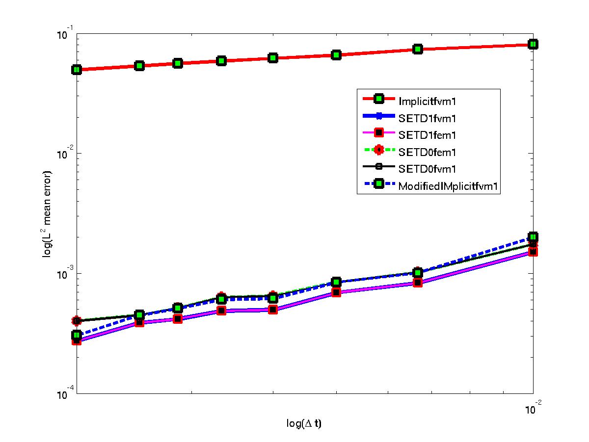
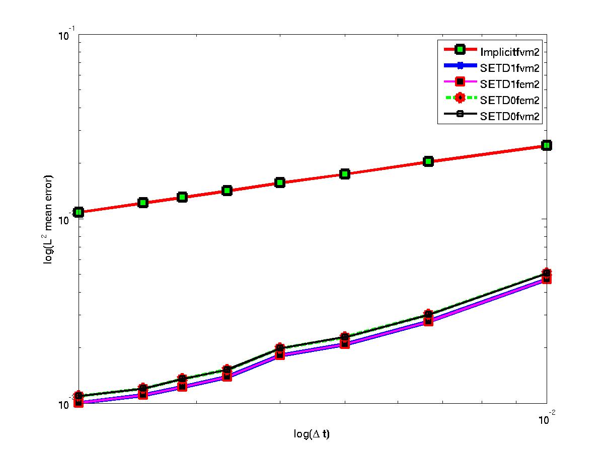
(a)                                                                 (b)

Figure 1. Convergence in the root mean square $L^{2}$ norm at $T=1$ as a function of $\Delta t$ with $H^{r}$, $r=1,2$. (a) Shows convergence for finite element and finite volume discretizations with $r=1$, $D=1$, $\lambda=1$, $\Gamma=1$ and $\Delta x=\Delta y=1/100$. In (b) we show convergence for finite element and finite volume discretizations with $r=2$, $D=1/100$, $\lambda=1$, $\Gamma=1$, $\Delta x=\Delta y=1/400$ (small to have a good look of convergence). The initial data is $X_{0}=0$ and the simulation is for (4.11) with 20 realizations.

In Figure 2 we show results with the exponential covariance function for the noise, as the noise is certainly in $H^{r},\;r=1\;\text{or}\;2$ we expect a rate of convergence close to one. The figure compares the finite element discretization for schemes (SETD0) and (SETD1) against the standard implicit scheme. The temporal order of convergence of the schemes (SETD0) is $0.80$ and (SETD1) is $1.05$ and $0.80$ for standard implicit scheme. We see the improved accuracy in the schemes (SETD0) and (SETD1) comparing to the standard implicit. We also see the better accuracy of the scheme (SETD1) compared to (SETD0).

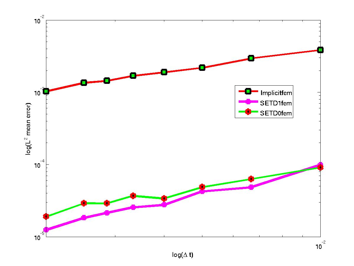
Figure 2. Convergence in the root mean square $L^{2}$ norm at $T=1$ as a function of $\Delta t$ with exponential covariance function with $D=1$, $\lambda=0.5$, $\Gamma=1$ and regular mesh coming from rectangular grid with size $\Delta x=\Delta y=1/100$. The simulation is for (4.11) with correlation lengths $b_{1}=b_{2}=0.2$ and 10 realizations. Initial data is given by $X_{0}=0$.

4.2. Stochastic advection diffusion reaction

As a more challenging example we consider the stochastic advection diffusion reaction SPDE

(4.12) $$dX=\left(D\varDelta X-\nabla\cdot(\textbf{q}X)-\frac{X}{X+1}\right)dt+dW,$$

with mixed Neumann-Dirichlet boundary conditions. and constant velocity $\textbf{q}=(1,0)$ for homogeneous medium. In terms of equation (1.1) the nonlinear term $F$ is given by

(4.13) $$F(u)=-\nabla\cdot(\textbf{q}u)-\frac{u}{(u+1)},\quad u\in\mathbb{R}^{+}$$

and clearly satisfies Assumption 3 (b). For heterogeneous medium we used three parallel high permeability streaks. This could represent for example a highly idealized fracture pattern. We obtain the Darcy velocity field q by solving the system

(4.16) $$\left\{\begin{array}[]{l}\nabla\cdot\underline{\mathbf{q}}=0\\ \b{q}=-\dfrac{k(\b{x})}{\mu}\nabla p,\end{array}\right.$$

with Dirichlet boundary conditions $\Gamma_{D}^{1}=\left\{0,1\right\}\times\left[0,1\right]\text{and Neumann boundary}\quad\Gamma_{N}^{1}=\left(0,1\right)\times\left\{0,1\right\}$ such that

$$p = \left\{\begin{array}[]{l}1\quad\text{in}\quad\left\{0\right\}\times\left[0,1\right]\\ 0\quad\text{in}\quad\left\{L_{1}\right\}\times\left[0,1\right]\end{array}\right.$$

and

$$-k\,\nabla p(x,t)\,\cdot\b{n}=0\quad\text{in}\quad\Gamma_{N}^{1}$$

where $p$ is the pressure, $\mu$ is dynamical viscosity and $k$ the permeability of the porous medium. We have assumed that rock and fluids are incompressible and sources or sinks are absent, thus the equation

(4.18) $$\nabla\cdot\underline{\mathbf{q}}=\nabla\cdot\left[\dfrac{k(\b{x})}{\mu}\nabla p\right]=0$$

comes from mass conservation.

To deal with high Péclet flows we discretize in space using finite volumes. Simulations are in $L^{2}(\Omega)$ since the discrete $L^{2}(\Omega)$ norm is easy to implement for all types of boundary conditions. We can write the semi-discrete finite volume method as

(4.19) $$dX^{h}=(A_{h}X^{h}+P_{h}F(X^{h})+b(X^{h}))+P_{h}P_{N}dW,$$

where here $A_{h}$ is the space discretization of $D\varDelta$ using only homogeneous Neumann boundary conditions and $b(X^{h})$ comes from the approximation of diffusion flux at the Dirichlet boundary condition size.

We compute the exponential functions $\varphi_{i}$ with Krylov subspace technique with dimension $m=6$ and the absolute tolerance $10^{-6}$ and the real fast Léja points technique for $\varphi_{0}$. In Figure 3 we shows the convergence of schemes (SETD0), (SETD1) and standard implicit scheme with $H^{2}$ noise for homogeneous medium, the ’true solution’ is the numerical scheme with smaller time step $\Delta t=1/15360$. All the schemes have $1/4$ for temporal order of convergence. We can also observe the accuracy of the scheme (SETD1) and (SETD0) comparing to and standard implicit scheme in Figure 3. In Figure 4 we shows the convergence of schemes (SETD0), (SETD1) with $H^{2}$ noise for heterogeneous medium. The two schemes have the same error. The corresponding mean of CPUtime for the scheme (SETD0) is given in Figure 4. We observe a slightly efficiency gain using the Léja points technique compared to the Krylov subspace technique during the evaluation of the action of $\varphi_{0}$.

In conclusion we obtained superior convergence for the stochastic exponential integrators using linear functionals of the noise with a finite element discretization. Furthermore we have shown that these schemes that require the exponential of a non-diagonal matrix can be efficiently implemented for finite element and finite volume discretizations of realistic porous media flow with stochastic forcing.

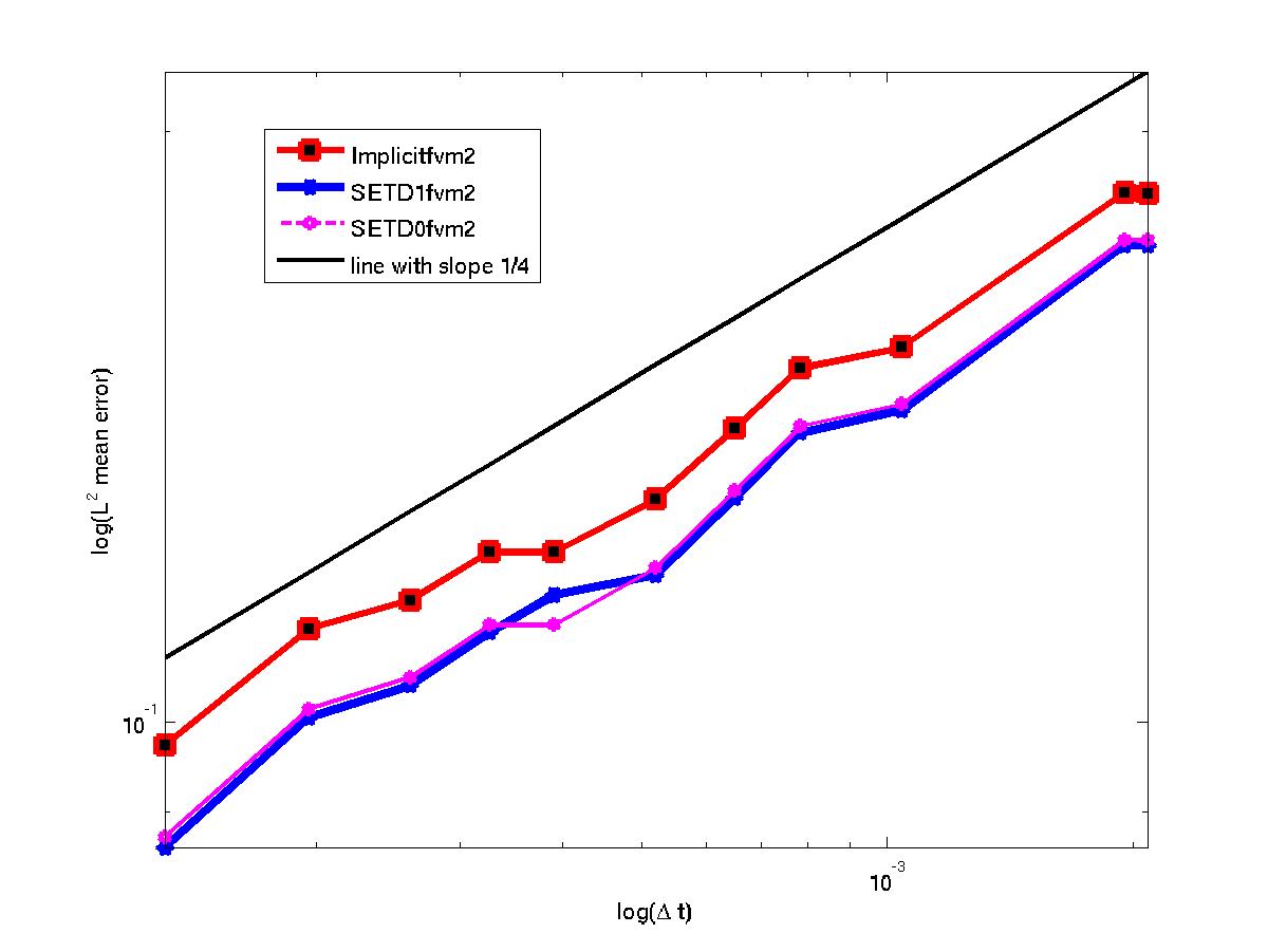
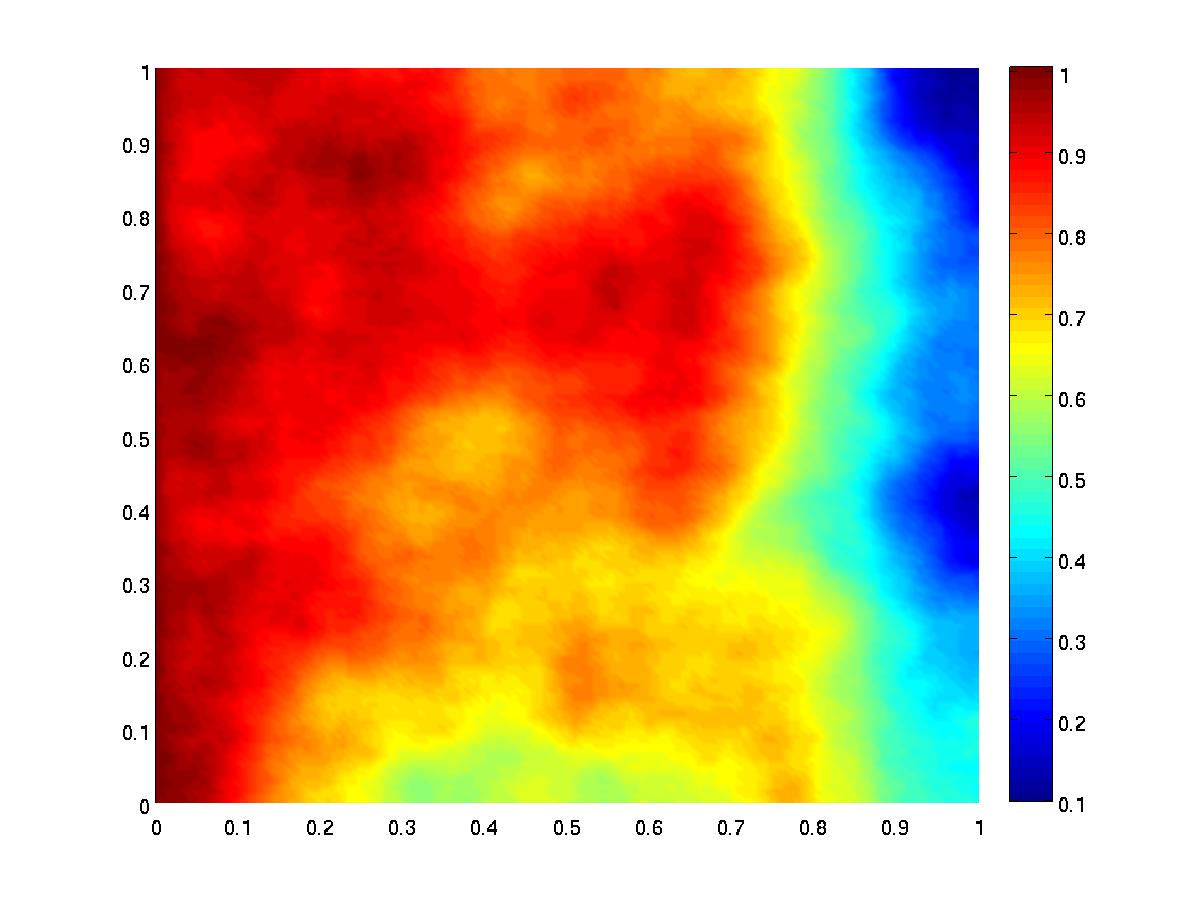
Figure 3. (a) Convergence of the root mean square $L^{2}$ norm at $T=1$ as a function of $\Delta t$ with 30 realizations with $\Delta x=\Delta y=1/160$, $X_{0}=0,\;\Gamma=0.01$ for homogeneous medium. The noise is white in time and in $H^{r}$ in space, $r=2$. The temporal order of convergence in time is $1/4$ for all schemes. In (b) we plot a sample ’true solution’ for $r=2$ with $\Delta t=1/15360$.

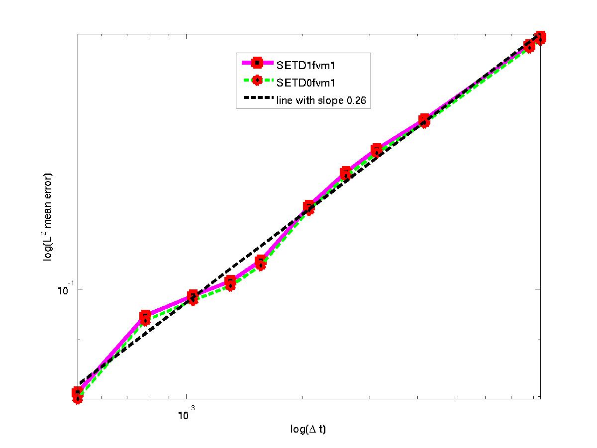
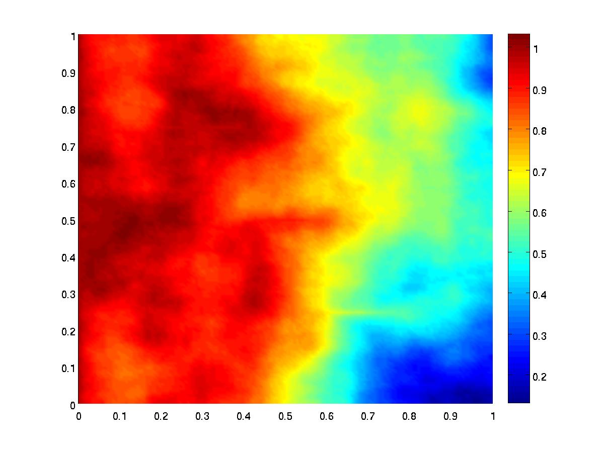
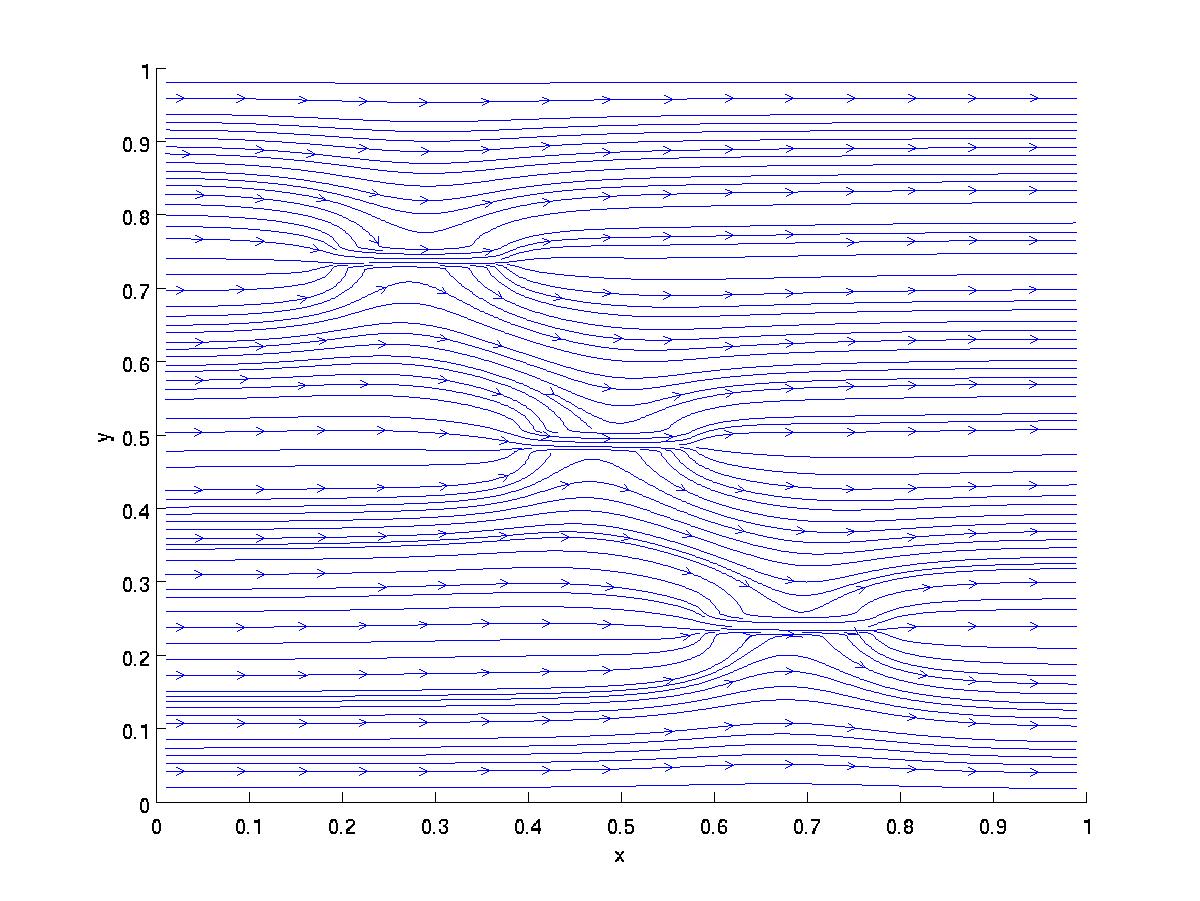
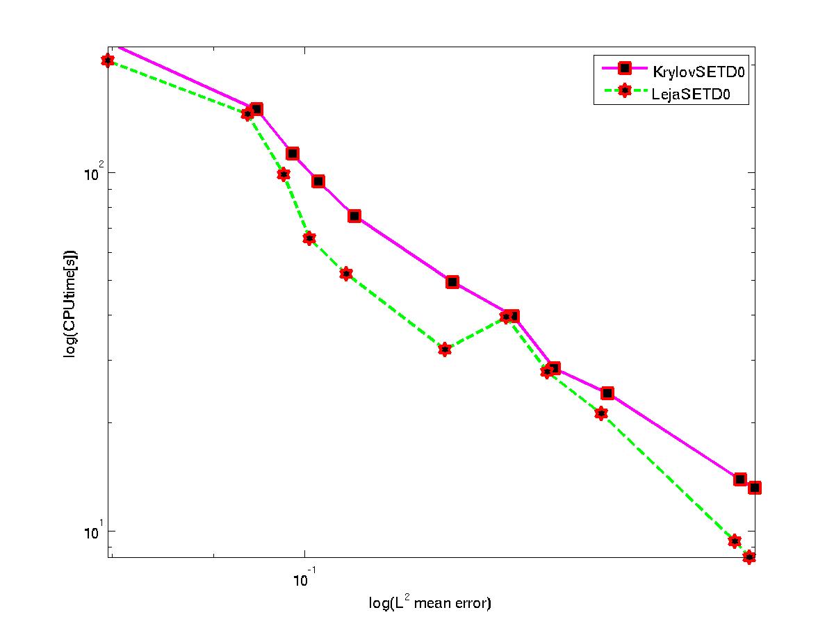
Figure 4. (a) Convergence of the root mean square $L^{2}$ norm at $T=1$ as a function of $\Delta t$ with 30 realizations and $\Delta x=\Delta y=1/160$, $X_{0}=0,\;\Gamma=0.01$ for heterogeneous medium. The noise is white in time and in $H^{r}$ in space, $r=2$. The temporal order of convergence in time is $0.26$ (close to $1/4$) for the two methods. In (b) we plot a sample ’true solution’ for $r=1$ with $\Delta t=1/15360$. In (c) we plot the streamline of the velocity field. In (d) the mean CPUtime for SETD0 using the Krylov and Leja points. The Péclet number for the flow is $16.58$.

References

- [1] G. J. Lord and A. Tambue. A modified semi–implict Euler-Maruyama scheme for finite element discretization of SPDEs. Submitted at SIAM Journal of Numerical Analysis, arXiv:1004.1998v1,2010.
- [2] A. Jentzen. High order pathwise numerical approximations of SPDES with additive noise. (unpublished manuscript), 2009.
- [3] A. Jentzen. Pathwise Numerical Approximations of SPDEs with Additive Noise under Non-global Lipschitz Coefficients. Potential Analysis, 31(4):375–404,2009.
- [4] A. Jentzen, and P. E. Kloeden. Overcoming the order barrier in the numerical approximation of SPDEs with additive space-time noise. Proc. R. Soc. A, 465(2102)(2009) 649–667.
- [5] A. Jentzen, P. E. Kloeden and G. Winkel. Efficient Simulation of Nonlinear parabolic SPDES with additive noise. Submitted to the Annals of Applied Probability , 2010.
- [6] E. Hausenblas. Approximation for semilinear stochastic evolution equations. Potential Analysis, 18(2)(2003) 141–186.
- [7] A. Jentzen, P. E. Kloeden and G. Winkel. Efficient Simulation of Nonlinear parabolic SPDES with additive noise. Submitted to the Annals of Applied Probability , 2010.
- [8] E. Hausenblas. Numerical analysis of semilinear stochastic evolution equations in Banach spaces. J. Comput. Appl. Math, 147(2) (2002) 485–516 .
- [9] I. Gyöngy. A note on Euler’s approximations. Potential Anal. , 8(3)(1998) 205-216 .
- [10] I. Gyöngy, and A. Millet. On discretization schemes for stochastic evolution equations. Potential Anal. ,23(2)(2005) 99-134 .
- [11] R. Eymard, T. Gallouet, and R. Herbin, Finite volume methods, in: P. G. Ciarlet, J. L. Lions (Eds.), Handbook of Numerical Analysis Volume 7, North-Holland, Amsterdam, 2000, pp. 713–1020.
- [12] P. Knabner and L. Angermann. Numerical methods for elliptic and parabolic partial differential equations solution. Springer, 2003.
- [13] D. Henry. Lecture Note in Mathematics: Geometric Theory of Semilinear Parabolic Equations. Springer, 840, 1981.
- [14] S. Larsson. Nonsmooth data error estimates with applications to the study of the long-time behavior of finite element solutions of semilinear parabolic problems. Preprint 1992-36, Department of Mathematics, Chalmers University of Technology, available at http://www.math.chalmers.se/stig/papers/index.html .
- [15] V. Thomée. Galerkin finite element methods for parabolic problems. Springer Series in Computational Mathematics, 1997.
- [16] H. Fujita, and T. Suzuki. Evolutions problems (part 1) in: P. G. Ciarlet, J. L. Lions (Eds.). Handbook of Numerical Analysis , vol II, North-Holland, Amsterdam, pp. 789–928, 1991 .
- [17] A. Tambue, G. J. Lord, and S. Geiger. An exponential integrator for advection-dominated reactive transport in heterogeneous porous media. Journal of Computational Physics ,229(10)(2010) 3957– 3969.
- [18] A. Tambue Efficient Numerical Methods for Porous Media Flow. Department of Mathematics, Heriot–Watt University, 2010.
- [19] P. Kloeden and G. J. Lord and A. Neuenkirch and T. Shardlow. The exponential integrator scheme for stochastic partial differential equations: Pathwise error bounds. Submitted to J. Comp. A. Math., 2009.
- [20] G. J. Lord, and T.Shardlow. Postprocessing for stochastic parabolic partial differential equations. SIAM J. Numer. Anal.,45(2) (2007) 870–889.
- [21] G. J. Lord and J. Rougemont. A numerical scheme for stochastic PDEs with Gevrey regularity. IMA J. Num. Anal.,24(4)(2004) 587–604 .
- [22] P.B. Bedient and H.S. Rifai and C.J. Newell. Ground Water Contamination: Transport and Remediation. Prentice Hall PTR , Englewood Cliffs, New Jersey 07632, 1994.
- [23] C.Prevot and M. Rockner. A Concise Course on Stochastic Partial Differential Equations. Springer, 2007.
- [24] G. Da Prato, and J. Zabczyk. Stochastic Equations in Infinite Dimensions. Encyclopedia of Mathematics and its Applications, 45 Cambridge University Press, 1992.
- [25] A. Pazy. Semigroups of linear operators and applications to partial differential equations. Applied Mathematical Sciences, Springer-Verlag, New York, 1983.
- [26] C. M. Elliott and S. Larsson. Error estimates with smooth and nonsmooth data for a finite element method for the Cahn-Hilliard equation. Math. Comp. , 58 (1992) 603–630.
- [27] Y. Yan. Semidiscrete Galerkin approximation for a linear stochastic parabolic partial differential equation driven by an additive noise. BIT, 44(4) (2004) 829–847.
- [28] T. Shardlow. Numerical simulation of stochastic PDEs for excitable media. J. Comput. Appl. Math,175(2)(2005) 429–446.
- [29] J. García-Ojalvo and J.M. Sancho. Noise in spatially extended systems. Institute for Nonlinear Science, Springer-Verlag, New York, 1999.
- [30] W. Luo. Wiener chaos expansion and numerical solutions of stochastic partial differential equations. California Institute of Technology ,Pasadena, California , 2006.
- [31] J. Baglama, D. Calvetti, and L. Reichel, Fast Léja points, Electron. Trans. Num. Anal. 7 (1998) 124–140.
- [32] L. Bergamaschi, M. Caliari, and M. Vianello, The RELPM exponential integrator for FE discretizations of advection-diffusion equations, in: M. Bubak, G. D. Van Albada, P. Sloot (Eds.), Lecture Notes in Computer Sciences Volume 3039, Springer Verlag, Berlin Heidelberg, 2004, pp. 434-442.
- [33] M. Hochbruck and C. Lubich, On Krylov subspace approximations to the matrix exponential operator, SIAM J. Numer. Anal. 34(5) (1997) 1911–1925.
- [34] R. B. Sidje, Expokit: A software package for computing matrix exponentials, ACM Trans. Math. Software 24(1) (1998) 130–156.
- [35] C. Moler and C. Van Loan, Ninteen Dubious Ways to Compute the Exponential of a Matrix, Twenty–Five Years Later, SIAM Review 45(1) (2003) 3–49.
- [36] A. Martinez, L. Bergamaschi, M. Caliari, and M. Vianello, A massively parallel exponential integrator for advection-diffusion models, J. Comput. Appl. Math. 231(1) (2009) 82–91.
- [37] L. Bergamaschi, M. Caliari, A. Martinez, and M. Vianello, Comparing Léja and Krylov approximations of large scale matrix exponentials, Comput. Sci. – ICCS 3994 (2006) 685–692.
- [38] H. Berland, B. Skaflestad, and W. Wright, A matlab package for exponential integrators, ACM Trans. Math. Software 33(1) (2007) Article No. 4
- [39] M. Caliari, M. Vianello, and L. Bergamaschi, Interpolating discrete advection diffusion propagators at Léja sequences, J. Comput. Appl. Math. 172(1) (2004) 79–99.
- [40] J. W. Thomas, Numerical partial differential equations: finite difference methods, Springer Verlag, Berlin Heidelberg New York, 1995.
- [41] L. Reichel. Newton interpolation at Leja points. BIT , 30(2)(1990) 332–346.
- [42] A. McCurdy, K. C. Ng, and B. N. Parlett. Accurate computation of divided differences of the exponential function. Math. Comp., 43(186)(1984) 501–528.