An Empirical Study of the Manipulability of Single Transferable Voting

Abstract

Voting is a simple mechanism to combine together the preferences of multiple agents. Agents may try to manipulate the result of voting by mis-reporting their preferences. One barrier that might exist to such manipulation is computational complexity. In particular, it has been shown that it is NP-hard to compute how to manipulate a number of different voting rules. However, NP-hardness only bounds the worst-case complexity. Recent theoretical results suggest that manipulation may often be easy in practice. In this paper, we study empirically the manipulability of single transferable voting (STV) to determine if computational complexity is really a barrier to manipulation. STV was one of the first voting rules shown to be NP-hard. It also appears one of the harder voting rules to manipulate. We sample a number of distributions of votes including uniform and real world elections. In almost every election in our experiments, it was easy to compute how a single agent could manipulate the election or to prove that manipulation by a single agent was impossible.

1 INTRODUCTION

Agents may try to manipulate an election by mis-reporting their preferences in order to get a better result for themselves. The Gibbard Satterthwaite theorem proves that, under some simple assumptions, there will always exist situations where such manipulation is possible [21, 25]. In an influential paper [3], Bartholdi, Tovey and Trick proposed an appealing escape: perhaps it is computationally so difficult to find a successful manipulation that agents have little option but to report their true preferences? To illustrate this idea, they demonstrated that the second order Copeland rule is NP-hard to manipulate. Shortly after, Bartholdi and Orlin proved that the more well known Single Transferable Voting (STV) rule is NP-hard to manipulate [2]. A whole subfield of social choice has since grown from this proposal, proving that various voting rules are NP-hard to manipulate under different assumptions.

Our focus here is on the manipulability of the STV rule. Bartholdi and Orlin argued that STV is one of the most promising voting rules to consider in this respect:

“STV is apparently unique among voting schemes in actual use today in that it is computationally resistant to manipulation.” (page 341 of [2]).

Whilst there exist other voting rules which are NP-hard to manipulate, computational complexity is either restricted to somewhat obscure voting rules like second order Copeland or to more well known voting rules but with the rather artificial restriction that there are large weights on the votes. STV is the only commonly used voting rule that is NP-hard to manipulate without weights. STV also appears more difficult to manipulate than many other rules. For example, Chamberlain studied [5] four different measures of the manipulability of a voting rule: the probability that manipulation is possible, the number of candidates who can be made to win, the coalition size necessary to manipulate, and the margin-of-error which still results in a successful manipulation. Compared to other commonly used rules like plurality and Borda, his results showed that STV was the most difficult to manipulate by a substantial margin. He concluded that:

“[this] superior performance …combined with the rather complex and implausible nature of the strategies to manipulate it, suggest that it [the STV rule] may be quite resitant to manipulation” (page 203 of [5]).

Unfortunately, the NP-hardness of manipulating STV is only a worst-case result and may not reflect the difficulty of manipulation in practice. Indeed, a number of recent theoretical results suggest that manipulation can often be computationally easy on average [8, 24, 31, 12, 32]. Such theoretical results typically provide approximation methods so do not say what happens with the complete methods studied here (where worst case behaviour is exponential). Most recently, Walsh has suggested that empirical studies might provide insights into the computational complexity of manipulation that can complement such theoretical results [30]. However, Walsh’s empirical study was limited to the simple veto rule, weighted votes and elections with only three candidates. In this paper, we relax these assumptions and consider the more complex multi-round STV rule, unweighted votes, and large numbers of candidates.

2 MANIPULATING STV

Single Transferable Voting (STV) proceeds in a number of rounds. We consider the case of electing a single winner. Each agent totally ranks the candidates. Unless one candidate has a majority of first place votes, we eliminate the candidate with the least number of first place votes. Any ballots placing the eliminated candidate in first place are re-assigned to the second place candidate. We then repeat until one candidate has a majority. STV is used in a wide variety of elections including for the Irish presidency, the Australian House of Representatives, the Academy awards, and many organizations including the American Political Science Association, the International Olympic Committee, and the British Labour Party.

Manipulate$(c,R,(s_{1},\ldots,s_{m}),f)$
1	if $|R|=1\mbox{\it\ \ \ \ \ \ \ \ \ \ \ \ \ \ \ \ \ \ \ \ \ \ \ \ \ \ \ \ \ \ \ \ \ \ \ \ \ \ \ \ ; Is there one candidate left?}$
2	then $\mbox{\bf return\ }(R=\{c\})\mbox{\it\ \ \ \ \ \ \ \ \ \ \ \ \ \ \ \ \ \ \ ; Is it the chosen candidate?}$
3	if $f=0\mbox{\it\ \ \ \ \ \ \ \ \ \ \ \ \ \ \ \ \ \ \ \ \ \ \ \ \ \ \ \ \ \ \ \ \ \ \ \ \ \ \ \ \ \ ; Is the top of the manipulator's vote currently free?}$
4	then
5	$\ignorespaces d\leftarrow arg\ min_{j\in R}(s_{j})\mbox{\it\ \ \ \ \ \ \ \ \ \ \ \ \ \ \ \ ; Who will currently be eliminated?}$
6	$\ignorespaces s_{d}\leftarrow s_{d}+w\mbox{\it\ \ \ \ \ \ \ \ \ \ \ \ \ \ \ \ \ \ \ \ \ \ \ \ \ \ ; Suppose the manipulator votes for them}$
7	$\ignorespaces e\leftarrow arg\ min_{j\in R}(s_{j})$
8	if $d=e\mbox{\it\ \ \ \ \ \ \ \ \ \ \ \ \ \ \ \ \ \ \ \ \ \ \ \ \ \ \ \ \ \ \ \ ; Does this not change the result?}$
9	then return
10	$\ignorespaces(c\neq d)\ and\ \mbox{\sc Manipulate}(c,R-\{d\},Transfer((s_{1},\ldots,s_{m}),d,R),0)$
11	else  return
12	$\ignorespaces((c\neq d)\ and\ \mbox{\sc Manipulate}(c,R-\{d\},Transfer((s_{1},\ldots,s_{m}),d,R),0))\ or$
13	$\ignorespaces((c\neq e)\ and\ \mbox{\sc Manipulate}(c,R-\{e\},Transfer((s_{1},\ldots,s_{m}),e,R),d))$
14	else                                              ; The top of the manipulator’s vote is fixed
15	$\ignorespaces d\leftarrow arg\ min_{j\in R}(s_{j})\mbox{\it\ \ \ \ \ \ \ \ \ \ \ \ \ \ \ \ \ ; Who will be eliminated?}$
16	if $c=d\mbox{\it\ \ \ \ \ \ \ \ \ \ \ \ \ \ \ \ \ \ \ \ \ \ \ \ \ \ \ \ \ \ \ \ \ ; Is this the chosen candidate?}$
17	then ${\mbox{\bf return\ }false}$
18	if $d=f\mbox{\it\ \ \ \ \ \ \ \ \ \ \ \ \ \ \ \ \ \ \ \ \ \ \ \ \ \ \ \ \ \ \ \ ; Is the manipulator free again to change the result?}$
19	then $\mbox{\bf return\ }\mbox{\sc Manipulate}(c,R-\{d\},Transfer((s_{1},\ldots,s_{m}),d,R),0)$
20	else  $\mbox{\bf return\ }\mbox{\sc Manipulate}(c,R-\{d\},Transfer((s_{1},\ldots,s_{m}),d,R),f)$

Figure 1: Our improved algorithm to compute if an agent can manipulate a STV election.

We use integers from $1$ to $m$ for the candidates, integers from $1$ to $n$ for the agents (with $n$ being the manipulator), $c$ for the candidate who the manipulator wants to win, $R$ for the set of un-eliminated candidates, $s_{j}$ for the weight of agents ranking candidate $j$ first amongst $R$, $w$ for the weight of the manipulator, and $f$ for the candidate most highly ranked by the manipulator amongst $R$ (or $0$ if there is currently no constraint on who is most highly ranked). The function $Transfer$ computes the a vector of the new weights of agents ranking candidate $j$ first amongst $R$ after a given candidate is eliminated. The algorithm is initially called with $R$ set to every candidate, and $f$ to $0$.

STV is NP-hard to manipulate by a single agent if the number of candidates is unbounded and votes are unweighted [2], or by a coalition of agents if there are 3 or more candidates and votes are weighted [9]. Coleman and Teague give an enumerative method for a coalition of $k$ unweighted agents to compute a manipulation of the STV rule which runs in $O(m!(n+mk))$ time where $n$ is the number of agents voting and $m$ is the number of candidates [7]. For a single manipulator, Conitzer, Sandholm and Lang give an $O(n1.62^{m})$ time algorithm (called CSL from now on) to compute the set of candidates that can win a STV election [9].

In Figure 1, we give a new algorithm for computing a manipulation of the STV rule which improves upon CSL in several directions First, our algorithm ignores elections in which the chosen candidate is eliminated. Second, our algorithm terminates search as soon as a manipulation is found in which the chosen candidate wins. Third, our algorithm does not explore the left branch of the search tree when the right branch gives a successful manipulation.

	CSL algorithm		Improved algorithm
$n$	nodes	time/s	nodes	time/s
2	1.46	0.00	1.24	0.00
4	3.28	0.00	1.59	0.00
8	11.80	0.00	3.70	0.00
16	59.05	0.03	12.62	0.01
32	570.11	0.63	55.20	0.09
64	14,676.17	33.22	963.39	3.00
128	8,429,800.00	6,538.13	159,221.10	176.68

Table 1: Comparison between the CSL algorithm and our improved algorithm to compute a manipulation of a STV election.

To show the benefits of these improvements, we ran an experiment in which $n$ agents vote uniformly at random over $n$ possible candidates. The experiment was run in CLISP 2.42 on a 3.2 GHz Pentium 4 with 3GB of memory running Ubuntu 8.04.3. Table 1. gives the mean nodes explored and runtime needed to compute a manipulation or prove none exists. Median and other percentiles display similar behaviour. We see that our new method can be more than an order of magnitude faster than CSL. In addition, as problems get larger, the improvement increases. At $n=32$, our method is nearly 10 times faster than CSL. This increases to roughly 40 times faster at $n=128$. These improvements reduce the time to find a manipulation on the largest problems from several hours to a couple of minutes.

3 UNIFORM VOTES

We start with one of the simplest possible scenarios: elections in which each vote is equally likely. We have one agent trying to manipulate an election of $m$ candidates where $n$ other agents vote. Votes are drawn uniformly at random from all $m!$ possible votes. This is the Impartial Culture (IC) model.

3.1 VARYING THE AGENTS

In Figures 2 and 3, we plot the probability that a manipulator can make a random agent win, and the cost to compute if this is possible when we fix the number of candidates but vary the number of agents in the election. In this and subsequent experiments, we tested 1000 problems at each point. Unless otherwise indicated, the number of candidates and of agents are varied in powers of 2 from 1 to 128.

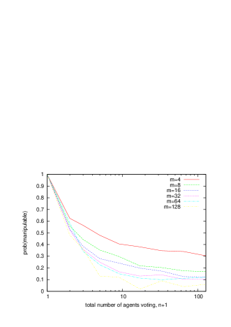
Figure 2: Manipulability of random uniform votes. The number of candidates is fixed and we vary the number of agents.

The ability of an agent to manipulate the election decreases as the number of agents increases. Only if there are few votes and few candidates is there a significant chance that the manipulator will be able to change the result. Unlike domains like satisfiability [22, 16], constraint satisfaction [15, 14], number partitioning [18, 20] and the traveling salesperson problem [19], the probability curve does not appear to sharpen to a step function around a fixed point. The probability curve resembles the smooth phase transitions seen in polynomial problems like 2-coloring [1] and 1-in-2 satisfiability [29]. Note that as elsewhere, we assume that ties are broken in favour of the manipulator. For this reason, the probability that an election is manipulable is greater than $\frac{1}{m}$.

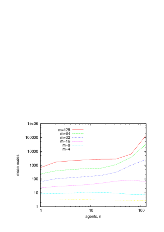
Figure 3: Search to compute if an agent can manipulate an election with random uniform votes. The number of candidates is fixed and we vary the number of agents.

Finding a manipulation or proving none is possible is easy unless we have both a a large number of agents and a large number of candidates. However, in this situation, the chance that the manipulator can change the result is very small.

3.2 VARYING THE CANDIDATES

In Figures 4, we plot the search to compute if the manipulator can make a random agent win when we fix the number of agents but vary the number of candidates. The probability curve that the manipulator can make a random agent win resembles Figure 2.

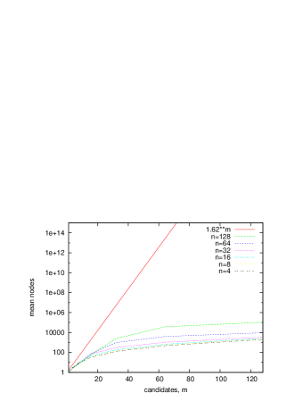
Figure 4: Search to compute if an agent can manipulate an election with random uniform voting. The number of agents is fixed and we vary the number of candidates.

Whilst the cost of computing a manipulation increases exponential with the number of candidates $m$, the observed scaling is much better than the $1.62^{m}$. We can easily compute manipulations for up to 128 candidates. Note that $1.62^{m}$ is over $10^{26}$ for $m=128$. Thus, we appear to be far from the worst case. We fitted the observed data to the model $ab^{m}$ and found a good fit with $b=1.008$ and a coefficient of determination, $R^{2}=0.95$.

4 URN MODEL

In many real life situations, votes are not completely uniform and uncorrelated with each other. What happens if we introduce correlation between votes? Here we consider random votes drawn from the Polya Eggenberger urn model [4]. We also observed very similar results when votes are drawn at random which are single peaked or single troughed. In the urn model, we have an urn containing all $m!$ possible votes. We draw votes out of the urn at random, and put them back into the urn with $a$ additional votes of the same type (where $a$ is a parameter). As $a$ increases, there is increasing correlation between the votes. This generalizes both the Impartial Culture model ($a=0$) and the Impartial Anonymous Culture ($a=1$) model. To give a parameter independent of problem size, we consider $b=\frac{a}{m!}$. For instance, with $b=1$, there is a 50% chance that the second vote is the same as the first.

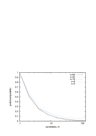
Figure 5: Manipulability of correlated votes. The number of agents is fixed and we vary the number of candidates. The $n$ fixed votes are drawn from the Polya Eggenberger urn model with $b=1$.

Figure 6: Search to compute if an agent can manipulate an election with correlated votes. The number of agents is fixed and we vary the number of candidates. The $n$ fixed votes are drawn using the Polya Eggenberger urn model with $b=1$. The curves for different $n$ fit closely on top of each other.

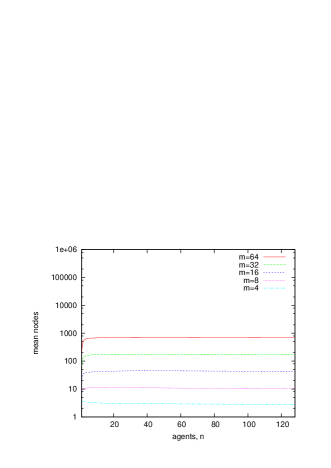
Figure 7: Search to compute if an agent can manipulate an election with correlated votes. The number of candidates is fixed and we vary the number of agents. The $n$ fixed votes are drawn using the Polya Eggenberger urn model with $b=1$.

In Figures 5 and 6, we plot the probability that a manipulator can make a random agent win, and the cost to compute if this is possible as we vary the number of candidates in an election where votes are drawn from the Polya Eggenberger urn model. The search cost to compute a manipulation increases exponential with the number of candidates $m$. However, we can easily compute manipulations for up to 128 candidates and agents. We fitted the observed data to the model $ab^{m}$ and found a good fit with $b=1.001$ and a coefficient of determination, $R^{2}=0.99$.

In Figure 7, we plot the cost to compute a manipulation when we fix the number of candidates but vary the number of agents. As in previous experiments, finding a manipulation or proving none exists is easy even if we have many agents and candidates. We also saw very similar results when we generated single peaked votes using an urn model.

5 COALITION MANIPULATION

Our algorithm for computing manipulation by a single agent can also be used to compute if a coalition can manipulate an election when the members of coalition vote in unison. This ignores more complex manipulations where the members of the coalition need to vote in different ways. Insisting that the members of the coalition vote in unison might be reasonable if we wish manipulation to have both a low computational and communication cost. In Figures 8 and 9, we plot the probability that a coalition voting in unison can make a random agent win, and the cost to compute if this is possible as we vary the size of the coalition. Theoretical results in [31] and elsewhere suggest that the critical size of a coalition that can just manipulate an election grows as $\sqrt{n}$. We therefore normalize the coalition size by $\sqrt{n}$.

Figure 8: Manipulability of an election as we vary the size of the manipulating coalition. The number of candidates is the same as the number of non-manipulating agents.

The ability of the coalition to manipulate the election increases as the size of the coalition increases. When the coalition is about $\sqrt{n}$ in size, the probability that the coalition can manipulate the election so that a candidate chosen at random wins is around $\frac{1}{2}$. The cost to compute a manipulation (or prove that none exists) decreases as we increase the size of the coalition. It is easier for a larger coalition to manipulate an election than a smaller one.

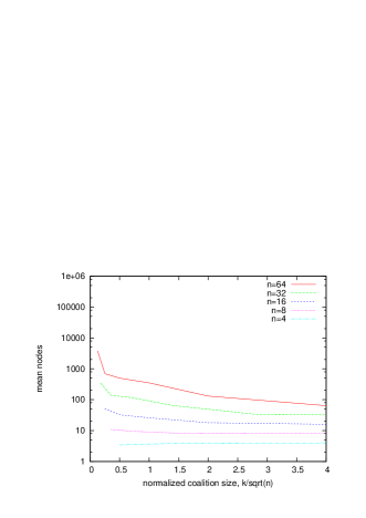
Figure 9: Search to compute if a coalition can manipulate an election as we vary coalition size.

These experiments again suggest different behaviour occurs here than in other combinatorial problems like propositional satisfiability and graph colouring [6, 26, 27, 28]. For instance, we do not see a rapid transition that sharpens around a fixed point as in 3-satisfiability [22]. When we vary the coalition size, we see a transition in the probability of being able to manipulate the result around a coalition size $k=\sqrt{n}$. However, this transition appears smooth and does not seem to sharpen towards a step function as $n$ increases. In addition, hard instances do not occur around $k=\sqrt{n}$. Indeed, the hardest instances are when the coalition is smaller than this and has only a small chance of being able to manipulate the result.

6 SAMPLING REAL ELECTIONS

Elections met in practice may differ from those sampled so far. There might, for instance, be some votes which are never cast. On the other hand, with the models studied so far every possible random/single peaked vote has a non-zero probability of being seen. We therefore sampled some real voting records [17, 13].

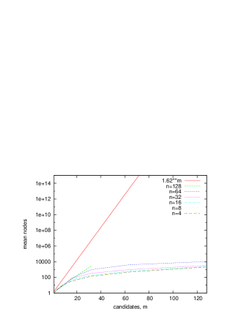
Figure 10: Search to compute if an agent can manipulate an election with votes sampled from the NASA experiment. The number of agents is fixed and we vary the number of candidates.

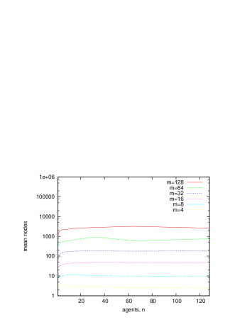
Figure 11: Search to compute if an agent can manipulate an election with votes sampled from the NASA experiment. The number of candidates is fixed and we vary the number of agents.

Our first experiment uses the votes cast by 10 teams of scientists to select one of 32 different trajectories for NASA’s Mariner spacecraft [11]. Each team ranked the different trajectories based on their scientific value. We sampled these votes. For elections with 10 or fewer agents voting, we simply took a random subset of the 10 votes. For elections with more than 10 agents voting, we simply sampled from the 10 votes with uniform frequency. For elections with 32 or fewer candidates, we simply took a random subset of the 32 candidates. Finally for elections with more than 32 candidates, we duplicated each candidate and assigned them the same ranking. Since STV works on total orders, we then forced each agent to break any ties randomly.

In Figures 10 to 11, we plot the cost to compute if a manipulator can make a random agent win as we vary the number of candidates and agents. Votes are sampled from the NASA experiment as explained earlier. The probability that the manipulator can manipulate the election resembles the probability curve for uniform random votes. The search needed to compute a manipulation again increases exponential with the number of candidates $m$. However, the observed scaling is much better than $1.62^{m}$. We can easily compute manipulations for up to 128 candidates and agents.

In our second experiment, we used votes from a faculty hiring committee at the University of California at Irvine [10]. We sampled from this data set in the same ways as from the NASA dataset and observed very similar results. It was easy to find a manipulation or prove that none exists. The observed scaling was again much better than $1.62^{m}$.

7 RELATED WORK

As indicated, there have been several theoretical results recently that suggest elections are easy to manipulate in practice despite NP-hardness results. For example, Procaccia and Rosenschein proved that for most scoring rules and a wide variety of distributions over votes, when the size of the coalition is $o(\sqrt{n})$, the probability that they can change the result tends to 0, and when it is $\omega(\sqrt{n})$, the probability that they can manipulate the result tends to 1 [23]. They also gave a simple greedy procedure that will find a manipulation of a scoring rule in polynomial time with a probability of failure that is an inverse polynomial in $n$ [24].

As a second example, Xia and Conitzer have shown that for a large class of voting rules including STV, as the number of agents grows, either the probability that a coalition can manipulate the result is very small (as the coalition is too small), or the probability that they can easily manipulate the result to make any alternative win is very large [31]. They left open only a small interval in the size for the coalition for which the coalition is large enough to manipulate but not obviously large enough to manipulate the result easily.

Friedgut, Kalai and Nisan proved that if the voting rule is neutral and far from dictatorial and there are 3 candidates then there exists an agent for whom a random manipulation succeeds with probability $\Omega(\frac{1}{n})$ [12]. Starting from different assumptions, Xia and Conitzer showed that a random manipulation would succeed with probability $\Omega(\frac{1}{n})$ for 3 or more candidates for STV, for 4 or more candidates for any scoring rule and for 5 or more candidates for Copeland [32].

Walsh empirically studied manipulation of the veto rule by a coalition of agents whose votes were weighted [30]. He showed that there was a smooth transition in the probability that a coalition can elect a desired candidate as the size of the manipulating coalition increases. He also showed that it was easy to find manipulations of the veto rule or prove that none exist for many independent and identically distributed votes even when the coalition was critical in size. He was able to identify a situation in which manipulation was computationally hard. This is when votes are highly correlated and the election is “hung”. However, even a single uncorrelated agent was enough to make manipulation easy again.

Coleman and Teague proposed algorithms to compute a manipulation for the STV rule [7]. They also conducted an empirical study which demonstrates that only relatively small coalitions are needed to change the elimination order of the STV rule. They observed that most uniform and random elections are not trivially manipulable using a simple greedy heuristic. On the other hand, our results suggest that, for manipulation by a single agent, a limited amount of backtracking is needed to find a manipulation or prove that none exists.

8 CONCLUSIONS

We have studied empirically whether computational complexity is a barrier to the manipulation for the STV rule. We have looked at a number of different distributions of votes including uniform random votes, correlated votes drawn from an urn model, and votes sampled from some real world elections. We have looked at manipulation by both a single agent, and a coalition of agents who vote in unison. Almost every one of the millions of elections in our experiments was easy to manipulate or to prove could not be manipulated. These results increase the concerns that computational complexity is indeed a barrier to manipulation in practice.

References

- [1] D. Achlioptas, Threshold phenomena in random graph colouring and satisfiability, Ph.D. dissertation, Department of Computer Science, University of Toronto, 1999.
- [2] J.J. Bartholdi and J.B. Orlin, ‘Single transferable vote resists strategic voting’, Social Choice and Welfare, 8(4), 341–354, (1991).
- [3] J.J. Bartholdi, C.A. Tovey, and M.A. Trick, ‘The computational difficulty of manipulating an election’, Social Choice and Welfare, 6(3), 227–241, (1989).
- [4] S. Berg, ‘Paradox of voting under an urn model: the effect of homogeneity’, Public Choice, 47, 377–387, (1985).
- [5] J.R. Chamberlin, ‘An investigation into the relative manipulability of four voting systems’, Behavioral Science, 30, 195–203, (1985).
- [6] P. Cheeseman, B. Kanefsky, and W.M. Taylor, ‘Where the really hard problems are’, in Proceedings of the 12th IJCAI, pp. 331–337. (1991).
- [7] T. Coleman and V. Teague, ‘On the complexity of manipulating elections’, in Proceedings of the 13th The Australasian Theory Symposium (CATS2007), pp. 25–33, (2007).
- [8] V. Conitzer and T. Sandholm, ‘Nonexistence of voting rules that are usually hard to manipulate’, in Proceedings of the 21st National Conference on AI. AAAI, (2006).
- [9] V. Conitzer, T. Sandholm, and J. Lang, ‘When are elections with few candidates hard to manipulate’, Journal of the Association for Computing Machinery, 54, (2007).
- [10] J.L. Dobra, ‘An approach to empirical studies of voting paradoxes: An update and extension.’, Public Choice, 41, 241–250, (1983).
- [11] J.S. Dyer and R.F. Miles, ‘An actual application of collective choice theory to the selection of trajectories for the Mariner Jupiter/Saturn 1977 project’, Operations Research, 24(2), 220–244, (1976).
- [12] E. Friedgut, G. Kalai, and N. Nisan, ‘Elections can be manipulated often’, in Proc. 49th FOCS. IEEE Computer Society Press, (2008).
- [13] I.P. Gent, H. Hoos, P. Prosser, and T. Walsh, ‘Morphing: Combining structure and randomness’, in Proceedings of the 16th National Conference on AI. AAAI, (1999).
- [14] I.P. Gent, E. MacIntyre, P. Prosser, B.M. Smith, and T. Walsh, ‘Random constraint satisfaction: Flaws and structure’, Constraints, 6(4), 345–372, (2001).
- [15] I.P. Gent, E. MacIntyre, P. Prosser, and T. Walsh, ‘Scaling effects in the CSP phase transition’, in 1st International Conference on Principles and Practices of Constraint Programming (CP-95), pp. 70–87. Springer-Verlag, (1995).
- [16] I.P. Gent and T. Walsh, ‘The SAT phase transition’, in Proceedings of 11th ECAI, ed., A G Cohn, pp. 105–109. John Wiley & Sons, (1994).
- [17] I.P. Gent and T. Walsh, ‘Phase transitions from real computational problems’, in Proceedings of the 8th International Symposium on Artificial Intelligence, pp. 356–364, (1995).
- [18] I.P. Gent and T. Walsh, ‘Phase transitions and annealed theories: Number partitioning as a case study’, in Proceedings of 12th ECAI, (1996).
- [19] I.P. Gent and T. Walsh, ‘The TSP phase transition’, Artificial Intelligence, 88, 349–358, (1996).
- [20] I.P. Gent and T. Walsh, ‘Analysis of heuristics for number partitioning’, Computational Intelligence, 14(3), 430–451, (1998).
- [21] A. Gibbard, ‘Manipulation of voting schemes: A general result’, Econometrica, 41, 587–601, (1973).
- [22] D. Mitchell, B. Selman, and H. Levesque, ‘Hard and Easy Distributions of SAT Problems’, in Proceedings of the 10th National Conference on AI, pp. 459–465. AAAI (1992).
- [23] A. D. Procaccia and J. S. Rosenschein, ‘Average-case tractability of manipulation in voting via the fraction of manipulators’, in Proceedings of 6th Intl. Joint Conference on Autonomous Agents and Multiagent Systems (AAMAS-07), pp. 718–720, (2007).
- [24] A. D. Procaccia and J. S. Rosenschein, ‘Junta distributions and the average-case complexity of manipulating elections’, Journal of Artificial Intelligence Research, 28, 157–181, (2007).
- [25] M. Satterthwaite, ‘Strategy-proofness and Arrow’s conditions: Existence and correspondence theorems for voting procedures and social welfare functions’, Journal of Economic Theory, 10, 187–216, (1975).
- [26] T. Walsh, ‘The Constrainedness Knife-edge’, in Proceedings of the 15th National Conference on AI. AAAI, (1998).
- [27] T. Walsh, ‘Search in a small world’, in Proceedings of 16th IJCAI. (1999).
- [28] T. Walsh, ‘Search on high degree graphs’, in Proceedings of 17th IJCAI. (2001).
- [29] T. Walsh, ‘From P to NP: COL, XOR, NAE, 1-in-k, and Horn SAT’, in Proceedings of the 17th National Conference on AI. AAAI, (2002).
- [30] T. Walsh, ‘Where are the really hard manipulation problems? the phase transition in manipulating the veto rule’, in Proceedings of 21st IJCAI. (2009).
- [31] Lirong Xia and Vincent Conitzer, ‘Generalized scoring rules and the frequency of coalitional manipulability’, in EC ’08: Proceedings of the 9th ACM conference on Electronic commerce, pp. 109–118, New York, NY, USA, (2008). ACM.
- [32] Lirong Xia and Vincent Conitzer, ‘A sufficient condition for voting rules to be frequently manipulable’, in EC ’08: Proceedings of the 9th ACM conference on Electronic commerce, pp. 99–108, New York, NY, USA, (2008). ACM.