Wind speed vertical distribution at Mt. Graham

Abstract

The characterization of the wind speed vertical distribution V(h) is fundamental for an astronomical site for many different reasons: (1) the wind speed shear contributes to trigger optical turbulence in the whole troposphere, (2) a few of the astroclimatic parameters such as the wavefront coherence time ($\tau_{0}$) depends directly on V(h), (3) the equivalent velocity $V_{0}$, controlling the frequency at which the adaptive optics systems have to run to work properly, depends on the vertical distribution of the wind speed and optical turbulence. Also, a too strong wind speed near the ground can introduce vibrations in the telescope structures. The wind speed at a precise pressure (200 hPa) has frequently been used to retrieve indications concerning the $\tau_{0}$ and the frequency limits imposed to all instrumentation based on adaptive optics systems, but more recently it has been proved that $V_{200}$ (wind speed at 200 hPa) alone is not sufficient to provide exhaustive elements concerning this topic and that the vertical distribution of the wind speed is necessary. In this paper a complete characterization of the vertical distribution of wind speed strength is done above Mt.Graham (Arizona, US), site of the Large Binocular Telescope. We provide a climatological study extended over 10 years using the operational analyses from the European Centre for Medium-Range Weather Forecasts (ECMWF), we prove that this is representative of the wind speed vertical distribution at Mt. Graham with exception of the boundary layer and we prove that a mesoscale model can provide reliable nightly estimates of V(h) above this astronomical site from the ground up to the top of the atmosphere ($\sim$ 20 km).

1 Introduction

The characterization of the wind speed above an astronomical site is extremely important for several different reasons. Firstly, because the wind speed is strictly correlated to the optical turbulence: strong wind speed and sharp wind speed gradients are indicators of a turbulent atmosphere, which in combination with a stable stratification of the atmosphere (a positive gradient of the potential temperature) creates optical turbulence that limits the resolution of the telescopes. Secondly, because the stronger the wind speed, the higher is the speed at which the turbulence layers cross the pupil of the telescope and the higher is the frequency at which adaptive optics systems are forced to work to correct the turbulence perturbations above the wavefront. Thirdly, because a too strong wind speed near the ground can introduce vibrations of the telescope structures.

At mid-latitudes, the wind speed varies with height showing a maximum at the jet stream level, usually 10-12 km (or $\sim$200 hPa) above sea level. The strength of the wind speed at high altitudes varies according to season, with the strongest values during (the local) winter and early spring (Masciadri & Garfias, 2001; Carrasco, Avila & Carramiñana, Carrasco et al.2005; García-Lorenzo et al., 2005; Masciadri & Egner, 2006; Egner, Masciadri & McKenna, Egner et al.2007; Bounhir et al., 2009; Masciadri et al., 2010). It has been observed that seasonal variations at the jet stream level are more pronounced at higher latitudes than at low latitudes in proximity of the equator (, Carrasco et al.2005) because of the general circulation of the wind speed at synoptic scale.

At extreme latitudes, i.e. in proximity of the poles, the wind speed is characterized by a completely different feature in the free atmosphere (Geissler & Masciadri, 2006; Sadibekova et al., 2006). It is rather weak up to 10 km and then increases monotonically above this height with a rate that increases with the distance of the site from the centre of the polar vortex (Hagelin et al., 2008). This assumption has been confirmed by Lascaux et al (2009).

Apart from the fact that a windy atmosphere more easily triggers optical turbulence, the astroclimatic parameter that directly depends not only on the optical turbulence but also on the wind speed is the wavefront coherence time:

$$\tau_{0}=0.057\lambda^{6/5}\Big{(}\int\limits_{0}^{\infty}{}V(h)^{5/3}C_{N}^{2}(h)dh\Big{)}^{-3/5}$$ (1)

also equivalent to:

$$\tau_{0}=0.31\frac{r_{0}}{V_{0}}$$ (2)

where $r_{0}$ is the Fried’s parameter and V₀ is the equivalent velocity:

$$V_{0}=\left(\frac{\int\limits_{0}^{\infty}{}V(h)^{5/3}C_{N}^{2}\left(h\right)dh}{\int\limits_{0}^{\infty}C_{N}^{2}dh}\right)^{3/5}$$ (3)

$\tau_{0}$ depends, therefore, on the vertical distribution of the wind speed V(h) and the optical turbulence $C_{N}^{2}\$(h). To simplify the calculation of the wavefront coherence time Sarazin & Tokovinin (2002) proposed a method to calculate $\tau_{0}$ using only the wind speed estimated at 200 hPa instead of the whole profile using an empirical relationship between $V_{0}$ and $V_{200}$: firstly they used $V_{0}=0.4*V_{200}$ and, in a second time, the expression has been modified in $V_{0}=max(V_{ground},0.4*V_{200})$. However, a few years ago (Masciadri & Egner, 2006), in a study done above San Pedro Mártir, it has been observed that the value of the constant 0.4 was not universal. The authors found the value 0.56 above San Pedro Mártir. However, they also proved that the relative error introduced in $\tau_{0}$ with the method of Sarazin & Tokovinin (2002), that does not consider the vertical distribution of the wind speed but just the wind speed in two precise regions of the atmosphere (near the ground and at 200 hPa), could be as great as 20$\%$-50$\%$, even using the appropriated constant. In other words, they proved that the proportionality between V₀ and V₂₀₀ is poorly reliable if one wishes precise estimates of $\tau_{0}$ (even if we select an appropriated constant). Masciadri & Egner (2006) concluded therefore that, for the calculation of the $\tau_{0}$, the vertical distribution of the wind speed on the whole troposphere is fundamental and necessary and the method suggested by Sarazin & Tokovinin (2002) can provide only some qualitative (but not accurate) estimates because it presents some intrinsic weak points. It appears therefore absolutely important in the field of the site characterization of an astronomical site, at least in cases such as the calculation of $\tau_{0}$, to characterize the wind speed vertical distribution. How to do that?

The estimate of the wind speed vertical distribution up to 20 km at an astronomical site (usually placed on the top of mountains) is not trivial. The Generalized Scidar, an optical instrument based on a remote sensing principle, can measure the wind speed (Avila, Vernin & Sanchez, 2001) at all the heights in which turbulent layers are present i.e. it can reconstruct a sort of vertical profile. Some estimates have been done in the past above different sites (Avila et al., 2006; , Egner et al.2007; Masciadri et al., 2010). However, this method requires the employment of an instrument that has to be placed at the focus of a telescope with a pupil size of at least 1.5 m and it can be performed for short periods (typically some tens of nights) related to dedicated experiments. Such an instrument is not suitable for routinely monitoring the wind speed or climatological studies. Alternatively wind speed profiles are routinely calculated by the General Circulation Models (GCM) (mainly from the ECMWF and NOAA/NCEP) and data-set can be retrieved in any site in the world with a horizontal resolution of 0.25 degrees (operational analyses) and 2.5 degrees (re-analyses). Both have been used for astronomical applications. More precisely, the ECMWF analyses have been used at mid-latitude sites (Masciadri & Garfias, 2001; , Egner et al.2007; Masciadri et al., 2010) as well as at extreme latitudes (Geissler & Masciadri, 2006; Hagelin et al., 2008). NOAA/NCEP re-analyses (vertical profiles) have been used at mid-latitude sites (, Carrasco et al.2005; Avila et al., 2006; Bounhir et al., 2009) and ERA-reanalyses of the ECMWF have been used at extreme latitudes (Sadibekova et al., 2006). Model outputs showed good correlations with measurements in all cases in which this has been calculated. The unique problem with analyses and re-analyses is that these estimates are representative of the wind speed above the astronomical site but not in the the surface and boundary layer where the local orographic effects have a major effect on the wind speed. Above roughly 1-2 km from the ground, the wind speed is almost horizontally homogeneous and the vertical distribution is basically the same with respect to a horizontal extension of some tens of kilometers. Below this height the analyses from the GCMs are less representative of the wind speed because their horizontal resolution is too low to give an accurate description of the interaction of the atmospheric flow with the topography near the surface.

However, in the surface (lowest few tens of meters) and boundary layers (typically the first kilometer above the surface) it has been proved (Masciadri, 2003) that mesoscale models, with a horizontal resolution of 1 km, can provide much better estimates than what analyses from the GCMs do above mid-latitude astronomical sites. In that paper the author proved that mesoscale models can provide estimates better correlated to measurements than analyses from GCM. It has also been proved that mesoscale models are able, contrary to the analyses from the GCMs, to discriminate the wind speed near the ground between two astronomical sites (Paranal and Maidanak) characterized by a median wind speeds that differ for 4-5 ms^-1. This study lets us think that mesoscale models could be a useful tool to reconstruct the wind speed vertical profile all along the 20 km from the ground. They are supposed to be comparable in performances to the ECMWF models above 1-2 km from the ground and they are supposed to provide better performances of the wind speed in the first 1-2 km from the ground.

In this paper we provide a climatological characterization of the wind speed above 1 km from the ground on the time scale of ten years using analyses from the ECMWF general circulation models and we investigate the possibility to use a mesoscale model to systematically reconstruct a complete wind speed vertical profile extended on the whole 20 km above Mt.Graham (Arizona, US) the site of the Large Binocular Telescope (LBT).

In Section 2 we use the operational ECMWF analyses over 10 years, 1998-2007, to present a climatological estimate of the median monthly wind speed. The operational data was chosen because of their higher resolution (0.25 degrees) with respect to the re-analyses. We will first prove the reliability of the ECMWF analyses in these regions of the world comparing analyses with radiosoundings launched in from Tucson International Airport ( $\sim$120 km from Mt. Graham).

In Section 3 we investigate the reliability of the wind speed vertical profiles retrieved from simulations with a mesoscale model (Meso-NH) in the high as well as in the low part of the atmosphere. The mesoscale model is run in a grid-nesting configuration covering a total surface of 800 km x 800 km and three imbricated models with 10, 2.5 and 0.5 km horizontal resolution (Table 1). The innermost model covering a surface of 60 km x 60 km. To estimate the model reliability we use measurements of the wind speed done by a Generalized Scidar run at the focus of the Vatican Advanced Technology Telescope (VATT) as well as by an anemometer located on the roof of the same telescope. This section aims to evaluate the possibility to use a mesoscale model to characterize the vertical distribution of the wind speed extending from the ground up to 20 km above astronomical sites. This should certainly represent an extremely valuable tool to provide an exhaustive monitoring of the wind speed above an astronomical site.

Table 1: Meso-NH model configuration. In the second column the horizontal resolution $\Delta$X, in the third column the number of grid points and in the fourth column the horizontal surface covered by the model domain.

	$\Delta$X (km)	Grid Points	Surface (km)
model 1	10	80 x 80	800 x 800
model 2	2.5	64 x 64	160 x 160
model 3	0.5	120 x 120	60 x 60

Finally, in Section 4, we present the conclusion of this study.

2 Monthly median wind speed

The ECMWF analyses used in this study are the operational analyses, downloaded from the MARS archive. For a more detailed description of the data-set we refer the reader to (Masciadri & Garfias, 2001; Geissler & Masciadri, 2006). As explained in the Introduction we only consider the wind speed above 1 km from the ground in this section.

In a previous study (, Egner et al.2007) done at Mt. Graham, it has been proved that independent measurements of the wind speed done at the summit of the mountain with a Generalized Scidar have a good and small relative discrepancy of the order of 23$\%$ with respect to the ECMWF analyses extracted from the nearest grid point. Similar results have been obtained above San Pedro Mártir by Avila et al. (2006).

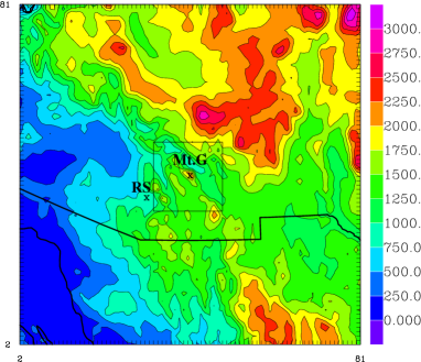
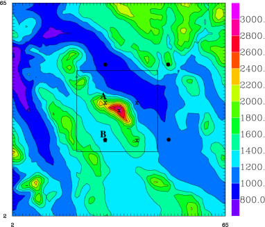
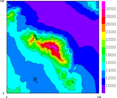
Figure 1: Top Left: Digital elevation map (DEM) of the Mt.Graham region (model 1 of Table 1 extended on 800 km x 800 km with $\Delta$X=10 km). The distance between the Mt. Graham summit and the Tucson Airport Station (label RS) is $\sim$ 120 km. The black square shows the location of model 2. Top Right: DEM (model 2 of Table 1 extended on 160 km x 160 km with $\Delta$X=2.5 km).The black square shows the location of the innermost model (model 3 of Table 1 extended on 60 km x 60 km with $\Delta$X=0.5 km). The location of the Mt.Graham Observatory is marked with an x on the summit of the mountain in the middle of the figure. The grid-points in which ECMWF analyses have been extracted (when the GCM resolution is 0.25$\degr$) are also marked with a x. The grid-points in which ECMWF analyses are extracted (when the GCM resolution is 0.5$\degr$) are marked with black dots. Bottom: DEM (model 3 of Table 1 extended on 60 km x 60 km with $\Delta$X=0.5 km).

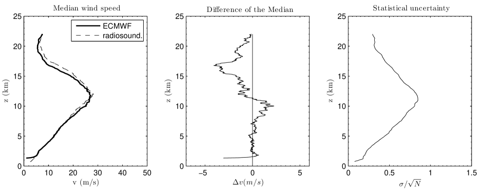
Figure 2: Left: median wind speed extended on the whole year 2005 calculated for the radiosoundings and the ECMWF analyses (see text). Centre: difference of the median wind speed (radiosoundings minus ECMWF analyses). Right: statistical uncertainty calculated for N=328, where N is the number of the nights for which we consider radiosoundings.

We try here a deeper analysis. The quality of the analyses in a region of the earth depends on how far/close are the meteorological stations with respect to the site one is studying and on the density of the measurements, i.e the number of the meteorological station in that particular region. In other words, it depends on the observations that have the most important weight in the data assimilation process of the GCMs for that region. The nearer to the astronomical site are the meteorological stations from which the radiosoundings are launched, the better is the quality of the analyses in proximity to the astronomical site. In order to make an estimate of how well the ECMWF analyses perform in the region of Mt.Graham we have made a comparison between the radiosoundings of the closest available meteorological station: Tucson airport (32.23$\degr$N, 110.96$\degr$W) at $\sim$120 km southwest from Mt.Graham (32.70$\degr$N, 109.89$\degr$W) (Fig.1-top left panel) and ECMWF analyses extracted from the closest grid point to the peak of Mt. Graham i.e. (32.75$\degr$N, 110.00$\degr$W) at $\sim$ 12 km north-west from the Mt. Graham peak (Fig.1-right panel, point with label (A)). The radiosoundings are available at 00:00 and 12:00 utc. We considered those at 12:00 utc corresponding to night time conditions at local time (12:00 utc equals 05:00 mst). Fig.2 shows the median wind speed vertical profile related to the whole year 2005 (left-panel), the difference of the median values (central-panel) and the statistical uncertainty $\sigma$/$\sqrt{N}$ that measures the accuracy of the measurements (right-panel). We observe that the difference of the median value is always very small (of the order of 1-2 ms^-1) in most part of the 20 km with a relative discrepancy less than or equal to 13$\%$. Only at 17 km the difference of the median values is somehow larger ($\sim$ 4 ms^-1). However, as can been seen in Fig.2-left panel, at this height the wind speed strength is almost 1/3 of the value assumed at the jet-stream level and it affects the integrated astroclimatic parameters in a less important way. In the calculation of the statistical uncertainty $\sigma/\sqrt{N}$, N $=$ 328 is the number of nights with radiosoundings available during 2005. We eliminated 37 nights for which the radiosoundings did not cover the whole 20 km above sea level. We conclude, therefore, that, above 1 km from the ground, the ECMWF analyses provide an accurate estimate of the wind speed and the wind speed vertical distribution is uniform on a horizontal scale of a few tens of kilometers.

Fig. 3 shows the monthly median vertical wind speed profile from the ECMWF-analyses for every month calculated on a time scale of ten years, from 1998 to 2007 at 06 utc (23 mst), from the ground up to 25 km. Considering the difference in altitude between the ECMWF grid-point ($\sim$ 1320 m) and the Mt. Graham summit (3200 m) we discuss these results for h $>$ 4 km above the sea level i.e. roughly 1 km above the ground of the highest location (Mt. Graham). The wind speed profiles calculated above Mt. Graham are characteristic of a mid-latitude site and the maximum of the wind speed is observed at 11-12 km above sea level. The wind speed maximum is located at the height of the jet-stream for the most part of the year. During July and August the wind speed at the jet-stream level is much weaker than during the other months and, in this period, the highest wind speed value is observed above 20 km, well into the stratosphere. The wind speed at the jet-stream level follows the classical sinusoidal seasonal trend in different periods of the year. Table 2 reports, for each month of the year, the average of the wind speed, the standard deviation for the yearly average values and the height corresponding to 200 hPa.

The wind speed at this height is characterized by values comparable to those observed above the major astronomical sites (, Carrasco et al.2005). The month with the strongest wind speed at 200 hPa is February (37.21 ms^-1), while the weakest wind speed is observed in July (11.17 ms^-1). The mean wind speed values as well as the standard deviation in each month appear very similar to that observed at San Pedro Mártir. This is not surprising considering that the two sites are located close to each other.

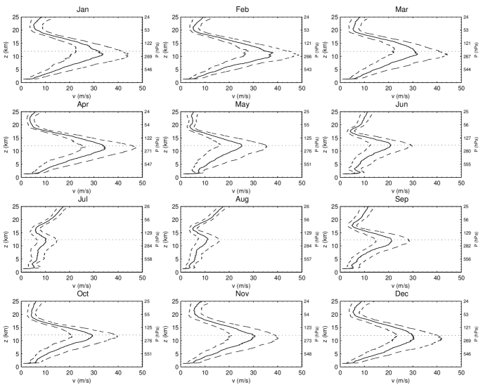
Figure 3: The median wind speed calculated with the ECMWF analyses for each month during 1998-2007 at Mt Graham, solid line. The dashed lines represent the first and third quartile. The dotted line indicates 200 hPa. Data-set are extracted from the grid point indicated with the label (A) in Fig.1-right panel.

Table 2: The mean wind speed at 200 hPa (200 mbar) at Mt Graham for the period 1998-2007. Column three and four are the standard deviation of the wind speed and the height corresponding to 200 hPa.

Month	Avg (ms-1)	std (ms-1)	h (km)
January	32.79	4.22	11.92
February	37.21	4.55	11.88
Mars	32.65	6.70	11.89
April	36.09	6.81	11.98
May	26.77	6.54	12.11
June	21.64	5.36	12.26
July	11.17	2.08	12.37
August	11.80	2.82	12.37
September	22.77	3.42	12.31
October	29.79	5.85	12.16
November	30.88	6.25	12.04
December	32.21	3.20	11.93
Average	27.06	4.82	12.10

The monthly median wind speed profile for each year is shown in Fig. 4. The difference between the individual years is smallest during the summer, when the strength of the wind speed is also the weakest, as is also indicated by the smaller difference between the first and the third quartiles observed for these months in Fig. 3. The greatest difference between individual years occurs during autumn (October and November) and spring (March and April). The difference between the calmest and the strongest yearly wind speed at the jet-stream level is over 20 ms^-1 during these months. This is coherent with the dispersion (dashed lines) indicated in Fig. 3. A peculiar pattern of alternating years with stronger and weaker winds is also found in October. The other months do not show this pattern, but there are clearly rather large differences in-between different years. This result indicates that studies on seasonal trends, for the wind speed and also the optical turbulence (that depends on the wind speed), should be preferably done on time scale of the order of some years to filter out effects due to this intrinsic variability that characterizes the wind speed in each month.

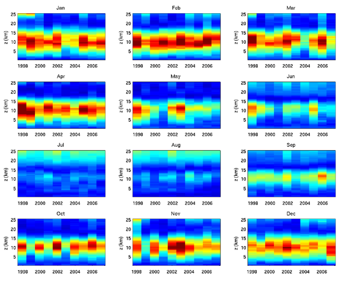
Figure 4: The temporal evolution of the annual median wind speed on the 1998-2007 period calculated with ECMWF analyses at Mt Graham. The color scale goes from 0 ms^-1 (blue) to 40 ms^-1 (dark red).

It is worth noting that the horizontal resolution of ECMWF-analyses, has changed during the studied period (1998-2007). During this period the horizontal resolution changed from 0.5 $\degr$ to 0.25$\degr$. Figure 1 shows the locations of the four grid points that are closest to Mt.Graham in the case of a resolution of 0.25$\degr$ (crosses) and 0.5$\degr$ (black points). With a horizontal resolution of 0.25$\degr$, the closest grid point to the peak of the mountain is A=(32.75$\degr$N, 110.00$\degr$W), located west-northwest of the peak. With a horizontal resolution of 0.5$\degr$ the closest grid point is B= (32.50$\degr$N, 110.00$\degr$W), southwest of the peak. A comparison of the vertical wind speed profile from both these grid points (see Appendix A) show that they are almost identical in the free atmosphere, therefore we consider that there are no problems of data inhomogeneity when we treat the average on time scale of the order of ten years.

3 The wind speed from the Meso-NH model

The Meso-NH is a non-hydrostatic mesoscale model developed jointly by Météo-France and Laboratoire d’Aérologie (Lafore et al., 1998). It is a grid point model based on the anelastic approximation that can simulate the temporal evolution in three dimensions of the classic meteorological parameters such as wind speed and direction, potential temperature and pressure.

For this study we have run the Meso-NH model in grid-nesting mode, using three two-way nested models, centered at the peak of Mt Graham. Details of the horizontal size and resolution of the three models are reported in Table  1. The outermost model covers an area of 800 x 800 km. The areas covered by the three models are shown in Fig. 1. The vertical grid is composed of 49 levels covering up to 20 km above sea level. The first vertical grid point is located at 20 m. Above we have a logarithmic stretching of 20% for the vertical grid size up to 3500 m. Above 3500 m the distance between the vertical levels is fixed and equal to 600 m.

The model is initialized with the analyses of the ECMWF, which also provides the boundary conditions for the outermost model. The runs start at 00:00 utc (17:00 mst), the synoptic hour closest to local evening, and last for 12 hours, to early morning in Arizona (05:00 mst). The first two hours are rejected to avoid the calculations being affected by spurious values due to the adaptation of the atmospheric flow to the ground. Data from the innermost model with the highest horizontal resolution (model 3) are treated here.

To ensure that the Meso-NH model can reconstruct reliable wind speed profile for h $\geq$ 1 km we compare the wind speed calculated by Meso-Nh with the wind speed calculated by the ECMWF analyses in the four grid points that surround Mt.Graham using the 0.25$\degr$ resolution (the four grid points are indicated with a x in Fig. 1). Figure 5 shows this comparison calculated for one night, May 21, 2005. The Meso-NH profiles are obtained by averaging the outputs calculated at each hour for the entire 10 hour simulation covering the period (17:00 to 05:00 mst). The ECMWF data are only available at the synoptic hours, therefore we considered the average of the ECMWF data at 00, 06 and 12 utc (at 17, 23 and 05 mst).

We observe that the wind speed profile from Meso-NH is very well correlated with the ECMWF analyses for all the four grid points above roughly 1 km from the ground. This also indicates that the wind speed is horizontally homogeneous over a surface of 0.25$\degr\times$0.25$\degr$.

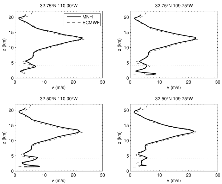
Figure 5: The vertical wind speed profile for the four grid points from the Meso-NH (solid line) and the ECMWF analyses (dashed line) that are located closest to Mt.Graham (grid points indicated with a cross in Fig.1), when using the 0.25°resolution. Calculations are done for the night May 21, 2005. The dotted line indicate the typical height below which the comparison makes no sense.

What is the Meso-NH ability in reconstructing the temporal evolution of the wind speed? To answer to this question we choose two nights, one characterized by a weak wind speed (May 29, 2007) and another characterized by a strong wind speed (February 26, 2008), and we compared the wind speed profiles calculated with the ECMWF analyses and the Meso-Nh model at the start and at the end of the simulation. We consider the wind speed calculated by the Meso-NH at the peak of Mt.Graham and the ECMWF wind speed extracted in the nearest grid point to the Mt. Graham summit. Again we are only interested, in this phase, in the wind speed above 1 km from the ground and, following the same logic we used in Section 2, we discuss the results obtained above 4 km from the sea level. Figure 6 shows the result of the comparison. ECMWF profiles are interpolated to the Meso-NH vertical grid points. Fig. 6-top and Fig. 6-bottom show, respectively, the start and the end of the simulation We observe that the wind speed profile calculated by Meso-Nh has evolved during both of the nights accordingly with the wind speed as calculated by the ECMWF. The shape of the profile is reasonably well correlated as well as the strength of the wind speed. We observe that the wind speed increases somewhat during the night on May 29, 2005 while decreases its strength on February 26, 2008. We conclude therefore that the mesoscale model is able to reconstruct the wind speed vertical distribution in the high part of the atmosphere and reproduces the spatio-temporal wind speed variability in a satisfactory way. In the case of May 29, 2007 (Fig. 6-bottom) the wind speed in the low part of the atmosphere reconstructed by the Meso-Nh model presents a few peaks that might be originated by the better horizontal resolution of the mesoscale model.

Figure 6: Vertical wind speed profile of the Meso-NH (solid line) and the ECMWF analyses (dashed line) at the beginning (00:00 UTC) and the end (12:00 UTC) of a simulation for two nights, May 29, 2007 (left hand side) and Feb. 26, 2008 (right hand side).

What about the ability of Meso-Nh in reconstructing the wind speed in the first kilometer from the ground? For this study we consider measurements provided by two different instruments: (1) measurements of the wind speed profile made with a Generalized Scidar (Masciadri et al., 2010) and related to 39 nights in different seasons (Table LABEL:tab2). (2) ’in situ’ measurements of the wind speed done with an anemometer located on the roof of the VATT ($\sim$ 20 m from the ground).

For these nights we can retrieve from the GS the wind speed along the whole 20 km. As already mentioned, a comparison of the Generalized Scidar wind speed profiles and the ECMWF analyses at Mt, Graham has been done in (Egner et al.2007) and it has been found a good correlation for h $\geq$ 1 km. Qualitative comparisons of the Generalized Scidar wind profiles with NCEP/NCAR re-analysis and wind speed from in situ balloons for 15 nights in May 2000 at San Pedro Mártir has been described in Avila et al. (2006). Also García-Lorenzo & Fuensalida (2006) compared the Generalized Scidar wind speed measurements done at the Teide Observatory with radiosoundings data launched by a meteorological station placed at $\sim$ 13 km away from the summit for four summer nights in 2003. However, to our knowledge, there is no detailed study of the reliability of the Generalized Scidar at describing the wind speed in the surface or boundary layer. For this reason, the measurements from an anemometer have been used to have an independent measurements in the very low atmosphere.

Table 3: Observing runs at Mt.Graham and the number of nights for which there are wind speed profiles from the GS.

Obs. runs (utc)	Nights
27 April 2005	1
20-26 May 2005	6
7-16 December 2005	5
28 May - 4 June 2007	8
17-29 October 2007	11
24 February - 4 March 2008	8

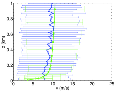
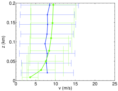
Figure 7: Left: Mean vertical profile of the wind speed in the boundary layer (1 km) obtained with the GS (blue line) and the Meso-NH (green line). The error-bars show the standard deviation. Right: zoom in the first 200 m.

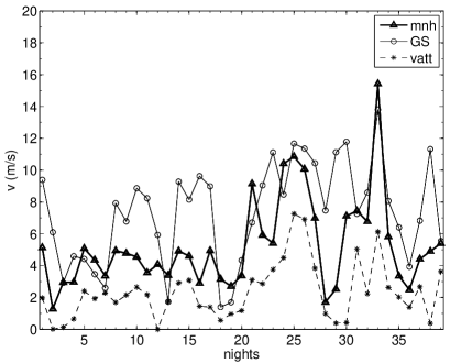
Figure 8: The average wind speed near the surface for Meso-NH (thick solid line and triangles) at h=20 m, an anemometer placed on the roof of the VATT at h $\sim$ 20m (dashed line and stars) and the Generalized Scidar (thin solid line and circles).

We have calculated the average wind speed vertical profile in the first kilometer for all 39 nights for which there are measurements of the wind speed from the Generalized Scidar (Fig. 7 - blue line) and compare the resulting profile with the average wind speed simulated by the Meso-NH for the same nights (Fig. 7 - green line). We remind that the GS is placed at the focus of the VATT therefore the first measurement (on the vertical grid) for the GS is at $\sim$ 20 m from the ground. Looking at Fig.7 we observe that, almost everywhere the two profiles are very well correlated, with the Generalized Scidar estimating wind speed that differs from the Meso-Nh model for not more than 1 ms^-1 all along the first kilometer from the ground. At 20 m the GS wind is slightly stronger than the wind calculated by the model. This is probably due to the fact that the GS measurements have a vertical error bar of the order of 25-30 m (see Masciadri et al. 2010) and the wind shear is particularly strong at this height. Therefore it might be that the higher wind speed detected by the GS at h =20 m can be originated by thin layers flowing at slightly higher distance from the dome and not resolved by the instrument. Figure 8 shows the average wind speed near the ground for every night reported in Table LABEL:tab2 in chronological order as measured by the Generalized Scidar and reconstructed by Meso-NH at around 20 m i.e. at the height of the dome of the telescope. In the same figure is also reported the wind speed measured in the same nights by the anemometer mounted on the top of the VATT. From a qualitative point of view, in Fig. 8 we observe that the temporal evolution of the wind speed reconstructed by the model during the 39 nights is very well correlated to the anemometer trend. The wind speed reconstructed by the model decreases and increases following the wind speed evolution measured by the anemometer in the same nights. Only a small off-set is present between the two estimates. From a quantitative point of view the mean wind speed from the GS at h = 20 m is 7.37 ms^-1, the mean wind speed reconstructed by the Meso-Nh model is 5.21 ms^-1, the mean wind speed measured by the anemometer is 2.44 ms^-1. The wind speed reconstructed by the model is well included in the range of the wind speed measurements and this certainly proves the reliability of the calculated wind speed. The weaker wind speed from the anemometer is probably due to the fact that the anemometer is an ’in situ’ measurement that is done well below the top of the trees. It has been observed in the past that the friction of the atmospheric flow with the trees causes a sharp and drastic decreasing of the wind speed below this height (something that is confirmed in the profile reconstructed by the model below 20 m).

We conclude therefore that the model provides reliable estimates all along the whole 20 km. In the future it would be good to be able to equip the observatory with anemometers located at different heights below and above the top of the trees preferably in open space environment so that the wind speed is not affected by the presence of buildings. This should permit us to better monitor the particular sharp change of wind speed in this region.

4 Conclusions

In this paper we aimed to give a complete characterization of the wind speed vertical distribution at Mt. Graham (Arizona, US) for astronomical applications. The simplest way of retrieving a complete characterization of the wind speed profile (with exception of the surface and boundary layer) is using the data from General Circulation Models (GCMs). In this study we use the operational analyses from the ECMWF extracted from the grid point closest to the peak of Mt. Graham, with a 0.25 degrees resolution, to study the vertical wind speed distribution over 10 years (1998-2007).

We have verified that the wind speed profile retrieved from the operational analyses of the ECMWF model is consistent with what is obtained by the radiosoundings from the nearby Tucson International airport. We also proved that the wind speed in this region is homogeneous with respect to horizontal spatial scales of the order of some tens of kilometers above $\sim$4 km from the sea level.

Having proved that the ECMWF analyses are reliable, we presented the monthly median wind speed extended on a 10 years time scale. The wind speed profiles are rather typical of a mid-latitude site with a pronounced wind speed maximum at the jet stream level (10-12 km above sea level) during most of the year. On the contrary, during the summer the maximum wind speed is located well into the stratosphere. The strongest variability (from different years) in the monthly median wind speed is found during spring and autumn.

For the same period we also provided the monthly mean wind speed values at 200 hPa, corresponding to the maximum wind speed values at the jet-stream height. The month with the strongest wind speed at 200 hPa is February (37.21 ms^-1), while the weakest wind speed is observed in July (11.17 ms^-1). Results indicate that the wind speed at the jet-stream level is very similar to what has been observed above the Observatory in San Pedro Mártir (Baja California) and it is consistent with the values observed above the best astronomical sites in the world.

Besides, we proved the reliability of a mesoscale model (Meso-Nh) in reconstructing the wind speed on the whole 20 km just above the summit of Mt. Graham included the boundary layer and the surface layer. We proved that the wind speed reconstructed by the model is very well correlated to the ECMWF analyses and it is also able to provide realistic profiles in the first kilometer from the ground.

The wind speed estimates from the mesoscale model have been compared to measurements from a Generalized Scidar and an anemometer located at 20 m from the ground on a sample of 39 nights. Above 50 m the wind speed profiles reconstructed by the model match in a very satisfactory way ($\Delta$V $\leq$ 1 ms^-1) with respect to the measured wind speed profiles. Closer to the surface, just in proximity of the top of the trees, the wind speed estimated by the model is included in the range of values given by the anemometer and the Generalized Scidar and for this reason can be considered satisfactory. However, the dispersion between the anemometer and the GS measurements seems a little too large. This difference is highly probably due to the fact the anemometer measures a wind speed that is not completely in free air (the anemometer is placed beside the dome of the VATT) and below the top of the trees. On the other side, the GS is probably affected by the wind speed just above the top of the trees because of its finite vertical resolution. The qualitative trend of the wind speed observed all along the sample of 39 nights is however very well reconstructed by the model and in agreement with measurements. The model appears to reconstruct very well the wind speed behavior above and below 20 m.

This paper therefore validates the Meso-Nh model as a tool to predict the wind speed vertical profile V(h) from the ground up to 20 km above Mt. Graham for each night and, at present time, it appears as the unique method to systematically estimate the whole wind speed vertical profile above an astronomical Observatory. We remind that it has been proved (Masciadri et al. 1999a, Masciadri & Jabouille, 2001, Masciadri et al. 2004, Lascaux et al. 2010) that Meso-Nh can provide reliable $C_{N}^{2}\$ profiles above an astronomical site and it appears therefore as an extremely useful tool for $\tau_{0}$ estimates. Besides there are evidences that it would be very useful to supply the Mt. Graham Observatory with anemometers located at different heights below and above the top of the trees ($\sim$ 20 m) because this should permit to provide a better constraints of the model for dedicated and more detailed applications.

Appendix A The wind speed at different horizontal resolution

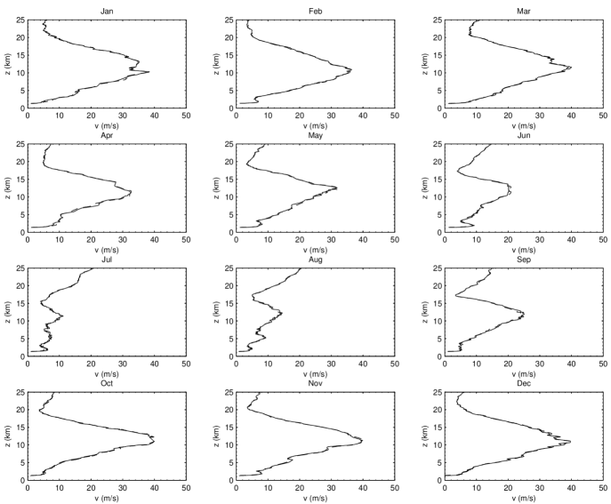
Figure 9: The median monthly wind speed for 2002 at the two different grid points closest to the peak of the mountain using 0.25$\degr$ resolution (32.75$\degr$N, 110.00$\degr$W) (solid lines) and 0.5$\degr$ resolution (32.50$\degr$N, 110.00$\degr$W) (dashed lines).

The horizontal resolution of the operational analyses of the ECMWF has changed during the ten year-period studied in this paper. This implies that the position of the closest grid points to Mt. Graham changes. The data in this study are downloaded from the 0.25$\degr$ resolution where the closest grid point to Mt. Graham is located east northeast of the mountain peak (Fig. 1 - point (A)) at 32.75$\degr$N, 110.00$\degr$W. Using the 0.5$\degr$ resolution the closest grid point is located 32.50$\degr$N, 110.00$\degr$W, southwest of the mountain (Fig. 1 - point (B)).

To closer examine which impact the different resolutions have on the vertical wind speed profile we have downloaded the data from both of these grid points for the entire year 2002. The monthly median wind speed profile is presented in Fig. 9, where the data from the grid point using the higher resolution (32.75$\degr$N, 110.00$\degr$W) is plotted with a solid line and the data from the 0.5$\degr$ resolution (32.50$\degr$N, 110.00$\degr$W) is plotted using a dashed line. The difference between the two data-sets is very small. During all months the lines overlap each other almost entirely. Some smaller offsets exist, but they are generally minor. The largest difference found, near the jet stream-level in October, is 2.8 ms^-1. We conclude therefore that the change in horizontal resolution in ECMWF-analyses during the 10 years did not introduce any biases in our calculation.

References

- Avila et al. (2001) Avila, R., Vernin, J., Sanchez, L., 2001, A&A, 369, 364
- Avila et al. (2006) Avila, R., Carrasco, E., Ibañez, F., Vernin, J., Prieur, J-L, Cruz, D. X., 2006, PASP, 118, 503
- Bounhir et al. (2009) Bounhir, A., Benkhaldoun, Z., Carrasco, E., Sarazin, M, 2009, MNRAS, 398, 862
- (4) Carrasco, E., Avila, R. & Carramiñana, 2005, PASP, 117, 104
- (5) Egner, S., Masciadri E., McKenna D, 2007, PASP, 119, 669
- García-Lorenzo & Fuensalida (2006) García-Lorenzo, B., Fuensalida, J. J, 2006, MNRAS, 372, 1483
- García-Lorenzo et al. (2005) García-Lorenzo, B., Fuensalida, J. J., Muñoz-Tuñon, C., Mendizalbal E., 2005, MNRAS, 356, 849
- García-Lorenzo et al. (2009) García-Lorenzo, B., Eff-Darwich, A., Fuensalida, J. J., Castro-Almazán, J., 2009, MNRAS, 397, 1633
- Geissler & Masciadri (2006) Geissler, K., Masciadri, E., 2006, PASP, 118, 1048
- Hagelin et al. (2008) Hagelin S., Masciadri E., Lascaux, F., Stoesz, J., 2008, MNRAS, 387, 1499
- Lafore et al. (1998) Lafore, J.-P., Stein, J., Asencio, N., Bougeault, P., Ducrocq, V., Duron, J., Fischer, C., Hereil, P., Mascart, P., Masson, V., Pinty, J.-P., Redelsperger, J.-L., Richard, E., Vilà-Guerau de Arellano, J., 1998, Annales Geophysicae, 16, 90
- Lascaux et al (2009) Lascaux, F., Masciadri, E., Hagelin, S., Stoesz, J., 2009, in Masciadri, E. & Sarazin, M.. eds., Optical Turbulence - Astronomy meets meteorology, Imperial College Press, p. 366
- Lascaux et al. (2010) Lascaux, F., Masciadri, E., Hagelin, S., 2010, MNRAS, 403, 1714
- Masciadri et al. (1999a) Masciadri, E., Vernin, J., Bougeault, P. 1999a A&ASS, 137, 185
- Masciadri and Jabouille (2001) Masciadri, E. & Jabouille, P., 2001, A&A, 376, 727
- Masciadri et al. (2004) Masciadri, E., Avila, R., Sanchez, L.J., 2004, RMxAA, 40, 3
- Masciadri (2003) Masciadri, E., 2003, RMxAA, 36, 249
- Masciadri & Egner (2006) Masciadri, E., Egner, S., 2006, PASP, 118, 1604
- Masciadri & Garfias (2001) Masciadri, E., Garfias T., A&A, 2001, 366, 708
- Masciadri et al. (2010) Masciadri, E., Stoesz, J., Hagelin, S., Lascaux, F., 2010, MNRAS, 404, 144
- Sadibekova et al. (2006) Sadibekova, T., Fossat, E., Genthon, C., Krinner, G., Aristidi, E., Agabi, K., Azouit, M., 2006, Antarct. Sci.,18, 437
- Sarazin & Tokovinin (2002) Sarazin, M., Tokovinin, A., 2002, in Vernet, E., Ragazzoni, R., Esposito, S., Hubin, N., eds, Proc. 58th ESO Conf. Workshop, Beyond Conventional Adaptive Optics, ESO Publications, Garching, p. 321