Exploiting translational invariance in Matrix Product State simulations of spin chains with periodic boundary conditions

Abstract

We present a matrix product state (MPS) algorithm to approximate ground states of translationally invariant systems with periodic boundary conditions. For a fixed value of the bond dimension $D$ of the MPS, we discuss how to minimize the computational cost to obtain a seemingly optimal MPS approximation to the ground state. In a chain of $N$ sites and correlation length $\xi$, the computational cost formally scales as $g(D,\xi/N)D^{3}$, where $g(D,\xi/N)$ is a nontrivial function. For $\xi\ll N$, this scaling reduces to $D^{3}$, independent of the system size $N$, making our algorithm $N$ times faster than previous proposals. We apply the method to obtain MPS approximations for the ground states of the critical quantum Ising and Heisenberg spin-$1/2$ models as well as for the noncritical Heisenberg spin-$1$ model. In the critical case, for any chain length $N$, we find a model-dependent bond dimension $D(N)$ above which the polynomial decay of correlations is faithfully reproduced throughout the entire system.

I Introduction

Concepts of entanglement for many-body quantum systems have recently proven useful to devise new methods for the numerical simulation of quantum spin chains. It has been shown that the very successful density matrix renormalization method (DMRG) White (1992) can be rephrased as a variational method over the class of matrix product states (MPS) Rommer and Östlund (1997); Vidal (2004); Verstraete et al. (2004, 2008); this realization clarified the relatively poor performance of DMRG for systems with periodic boundary conditions (PBC), as MPS with open boundary conditions (OBC) do not have the right entanglement structure. It was shown in Verstraete et al. (2004) how this could be cured by using a MPS with PBC. However, due to the cyclic structure of the underlying MPS, the computational cost of the simulation in terms of the MPS bond dimension $D$ grew from $O(D^{3})$ to $O(D^{5})$. This was subsequently lowered to $O(D^{3})$ in Sandvik and Vidal (2007); Pippan et al. (2010).

An important motivation to study finite chains is that one can compute bulk properties of the system in the thermodynamic limit by extrapolating results obtained for increasingly large chains Cardy (1996). In this context, it is relevant whether OBC or PBC are considered. For a finite chain with OBC, local expectation values differ from those in thermodynamic limit due both to finite-size effects and to boundary effects, and larger chains need to be considered. In contrast, with PBC only finite-size effects are present. This makes the extrapolation to the thermodynamic more transparent and smaller systems need to be simulated. Another important advantage of PBC is that only in this case a finite chain can be translation invariant (TI) . This is crucial feature for the present work, where TI is exploited in order to reduce the computational costs of simulating finite chains.

Pippan, White and Evertz Pippan et al. (2010) recently showed how to simulate spin chains with PBC with an MPS algorithm whose computational cost given in terms of $D$ scales like $O(D^{3})$. The intuition behind this scaling can be understood if one first considers systems with a correlation length $\xi$ that is much shorter than the system size $N$. Let us choose a block of sites with size $l$ such that $\xi>l$ (see figure  1a). In this case correlations between the left and the right ends of the block are mediated only through the sites inside the block. It is clear that the properties of this block are exactly the same as those of a block of equal length embeded in the bulk of a sufficiently large system with OBC. It is then not surprising that computing observables that are contained within the block has a cost proportional to $D^{3}$, as in the case of OBC. This is basically due to the fact that such calculations involve contracting a tensor network that has, as uncorrelated left and right boundary conditions, two boundary vectors with $D^{2}$ components Verstraete et al. (2008). Now imagine we are interested in the description of properties contained in a larger block such that $\xi>l>N-\xi$ (see figure 1b). This block is small enough for its ends to have correlations that are mediated via its own sites, yet large enough that correlations are also mediated via the sites outside the block, since now $N-l<\xi$. If these externally mediated correlations are relatively small, the situation is not very different from the previously described case where $l<N-\xi$. All we have to do is to replace the two uncorrelated boundary vectors with a low rank boundary matrix that contains the small amount of correlations. If the rank of the matrix is $n$, then the cost of this algorithm will be proportional to $nD^{3}$.

(a)  Medium $\xi$, small $l$: equivalent to OBC environment.

(b)  Medium $\xi$, medium $l$: equivalent to partially correlated OBC environment.

(c)  Large $\xi$, any $l$: equivalent to fully correlated OBC environment.

Figure 1: (Color online). The properties of a block of size $l$ within a PBC system can be equivalent to those of a block with same size in the bulk of an OBC system. Depending on $l$ and the correlation length $\xi$, the left and right boundary conditions of the OBC system are more or less correlated.

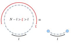
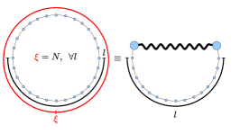
We emphasize two important aspects of the computational cost of the algorithm in Ref. Pippan et al. (2010). The first one is that the cost is also proportional to the system size $N$, due to the usual sweeping procedure that optimizes one site at each instant. We will show below how, in the case of a TI chain, one can get rid of this factor . This is achieved by using a TI MPS, where the $N$ tensors of the MPS are chosen to be identical. For all $D$, the precision of our results is comparable to that reported in Ref. Pippan et al. (2010). This indicates that restricting the MPS ansatz to be TI does not lead to a loss of precision, while yielding a substantial reduction of the computational cost. The second one is the multiplicative factor $n$ corresponding to the rank of the boundary matrix that transfers correlations between the ends of a block. In the case where the correlation length $\xi$ is of the order of the system size $N$ (see figure 1c), this factor may not be small. In a worst case scenario, where strong correlations between distant sites would force the boundary matrix to be full rank, i.e. $n=D^{2}$, the approach in Ref. Pippan et al. (2010) would not be better than the $O(D^{5})$ algorithm of Ref. Verstraete et al. (2004). Thus for critical systems where $\xi\approx N$ it is a priori unclear what the overall scaling of the computational cost in $D$ will be. However, in Ref. Pippan et al. (2010) it has been indicated that if $D$ is not too large, the ground state energy of a critical spin chain obtained using a small constant $n$ is satisfactory, in that its accuracy scales with $D$ in a similar way as it would in an OBC chain of the same size.

Here we shall show how to exploit TI to obtain a faster algorithm that, for instance, does not scale with $N$ when $\xi\ll N$. However, except for the case $\xi\ll N$, we still lack a precise characterization of how the cost scales as a function of $D$ and $N$. We benchmark the present approach by addressing both critical (i.e. $\xi\approx N$) and non-critical (i.e. $\xi\ll N$) chains. An important observation is that in the case of critical systems the finite bond dimension $D$ of the MPS introduces an effective correlation length $\tilde{\xi}_{D}\approx D^{\kappa}$ Nishino et al. (1996); Andersson et al. (1999); Tagliacozzo et al. (2008); Pollmann et al. (2009) that depending on $D$ can be much smaller than the actual one. This implies that as $N$ grows, a larger bond dimension $D\approx N^{1/\kappa}$ needs to be considered if correlations between distant sites of the chain with PBC are to be properly captured Our numerical results are consistent with a complex scenario where the cost of simulations is dominated by the crossover between finite-$N$ and finite-$D$ corrections, as further discussed in Pirvu et al. (2010).

The rest of the paper is structured as follows: we start by sketching the main idea of the approach in Sect. II, followed by an in-depth presentation of the algorithm in Sect. III. In Sect. IV we present numerical results for the critical Quantum Ising and Heisenberg spin-$1/2$ models as well as for the non-critical Heisenberg spin-$1$ model. Finally Sect. V contains some conclusions.

II Overview

This work is concerned with the approximation of ground states (GS) within the variational class of MPS with PBC defined in Verstraete et al. (2004). Since critical systems are arguably among the most challenging ones from a computational perspective, we will apply the approach to investigate critical spin chains (although non-critical chains can also be considered). An important restriction is that we only consider TI systems, which we will analyse with a TI MPS ansatz, namely an MPS where the tensors corresponding to different sites are all equal. The resulting variational class is a subclass of the one defined in Verstraete et al. (2004). The TI MPS with PBC reads

$$\ket{\psi(A_{i})}=\sum_{i_{1},\dots i_{N}=1}^{d}\mbox{Tr}\big{(}A_{i_{1}}A_{i_{2}}\dots A_{i_{N}}\big{)}\ket{i_{1}i_{2}\dots i_{N}}$$ (1)

with identical matrices $A_{i}$ at every site. Note that since for fixed $i$, each $A_{i}$ represents a matrix, the MPS is completely characterized by the three dimensional tensor $A_{i\phantom{\alpha}\beta}^{\phantom{i}\alpha}=:\mathbf{A}$. Furthermore we should point out that we will mostly be interested in Hamiltonians that are real and reflection invariant; these symmetries can be implemented at the level of MPS by choosing the matrices $A_{i}$ real and symmetric. This extra constraint does not seem to deteriorate the accuracy of the variational procedure.

Since our ansatz consists of $N$ copies of the same tensor, the energy is not a quadratic expression in the variables defined by the tensors $A_{i}$; this implies that we cannot use the sweeping procedure described in Verstraete et al. (2004) or any other procedure that lowers the energy by minimizing it for one site at a time. While this might seem a reason to be concerned at first, it will actually be the key to reducing computational costs.

The advantages of a TI MPS ansatz (with periodicity one or two) have already been exploited in the context of infinitely long chains White (1992); Nishino and Okunishi (1995); Vidal (2007); McCulloch (2008); Orús and Vidal (2008); Pirvu et al. (2010). Refs. White (1992); Nishino and Okunishi (1995); McCulloch (2008) used a TI MPS in the context of infinite system DMRG. In Ref. Vidal (2007), instead, a (two-site periodic) MPS approximation to ground states was obtained by imaginary time evolution. Refs. Orús and Vidal (2008); Pirvu et al. (2010) discussed how to compute ground states with a one-site TI MPS when the imaginary time evolution operator can be well enough approximated by layers of one-site TI matrix product operators. An attempt to adapt that method to finite chains with PBC yielded results that are not as accurate as one might expect . Finally, we also point out that a TI MPS with PBC was already used in Ref. Sandvik and Vidal (2007) together with Monte Carlo sampling techniques, with a formal cost $O(ND^{3})$. In that case, the use of sampling techniques reduced the cost from $O(D^{5})$ to $O(D^{3})$, but at the same time enforced the multiplicative factor $N$, since a TI MPS does not represent a TI state once a given configuration is chosen during the sampling.

An obvious way to find the TI-MPS with minimal energy is a multidimensional minimization procedure that requires only evaluations of the function itself, such as the downhill simplex method Press et al. (2007). When no further information about the function is available, this is indeed the method of choice. It is extremely robust but also extremely slow. However, if there is a feasible way to obtain more elaborate information such as the gradient or the Hessian, there are methods relying on these quantities that are clearly superior in what regards the speed of convergence and the required storage space.

In the following we will present an efficient algorithm to calculate the gradient of the energy $\nabla E(\mathbf{a})$ where the argument $\mathbf{a}=\mbox{vec}(\mathbf{A})$ denotes the vector containing all entries of the MPS tensor $\mathbf{A}$. The result will then be used by a standard numerical library conjugate gradient algorithm to find a minimum of $E(\mathbf{a})$. We must emphasize that this minimum is by no means guaranteed to be the global one i.e. the optimal ground state approximation within the subspace defined by our special MPS ansatz. However, our numerical results seem to be slightly more accurate than previous results Pippan et al. (2010), while we have obtained a reduction in computational costs. We will illustrate the accuracy of this approach by applying it to two exactly solvable models in order to give exact values for the numerical errors.

The computational cost will turn out to scale as $O(mnD^{3})+O(n^{2}D^{3})$ where $D$ is the virtual bond dimension and $m$ and $n$ are some parameters to be specified below. Briefly speaking, the scaling can be understood as follows: first we approximate large powers of the MPS transfer matrix, whose exact definition will be given later in the text, within a reduced subspace of dimension $n$. Treating each of the $n$ dimensions separately allows us to transform the contraction of a tensor network with PBC (which scales as $O(D^{5})$) into $n$ contractions of tensor networks with OBC (each of which scales as $O(D^{3})$). As we will explain in more detail in the next section, the resulting tensor networks will still contain at most one portion represented by say $m$ adjacent transfer matrices that is not connected to the already approximated one. If $m$ is large, this second portion can again be approximated within a $n$-dimensional subspace thereby yielding the scaling $O(n^{2}D^{3})$. If $m$ is small, we are forced to contract the transfer matrices one after the other which gives the scaling $O(mnD^{3})$.

III The algorithm

Let us rearrange the MPS tensor components in a vector $\mathbf{a}=\mbox{vec}(\mathbf{A})$ which allows us to write the energy as a function over the manifold of free parameters in the MPS

$$E(\mathbf{a})=\frac{\bra{\psi(\mathbf{a})}H\ket{\psi(\mathbf{a})}}{\braket{\psi(\mathbf{a})}{\psi(\mathbf{a})}}\equiv\frac{\bra{\psi(\mathbf{A})}H\ket{\psi(\mathbf{A})}}{\braket{\psi(\mathbf{A})}{\psi(\mathbf{A})}}\,\,\,.$$ (2)

Note that due to the constraints that the matrices are real and symmetric, the number of vector components in $\mathbf{a}$ has been reduced to $\frac{1}{2}dD(D+1)$. As we will treat only spin-1/2 chains (i.e. $d=2$) in this work, the variational parameter manifold is actually $D(D+1)$-dimensional. Furthermore we will denote expectation values taken with respect to the MPS defined by the tensor $\mathbf{A}$ as $\langle O\rangle_{\mathbf{A}}:=\bra{\psi(\mathbf{A})}O\ket{\psi(\mathbf{A})}$.

Also note that (2) can have local extrema as opposed to $E(\Psi)=\bra{\Psi}H\ket{\Psi}$ which is a convex quantity in the exponentially large Hilbert space. The MPS-parametrization restricts the full parameter space to a submanifold thus possibly generating local extrema where all derivatives in this subspace vanish. If one uses as a starting point of the conjugate gradient algorithm a random vector $\mathbf{a}_{rand}$, the search algorithm will typically get stuck in a local minimum. In order to avoid getting stuck in one of these, we will choose as a starting point a vector $\mathbf{a}_{0}$ of which we can be sure that it is close to the global minimum. This approach turns out to be very robust and fast. If we are interested in ground states of chains with very large $N$, the most natural choice for the starting vector is an MPS approximation of the GS of the same model in the thermodynamic limit. Note that this MPS must have exactly the same symmetry properties as our ansatz. It was shown in previous work Pirvu et al. (2010) how to obtain this MPS and we will actually use the tensors computed there as starting points for the present algorithm. It is obvious why the MPS for the GS of the infinite chain is a good choice if one is interested in finite PBC-chains with $N\gg\xi(D)$, where $\xi(D)$ is the correlation length induced by finite $D$. However, it turns out that this approach also works satisfactory for moderately large $N$. Of course, if there already is any PBC solution available, using that one as a starting point may provide a gain in convergence time, especially if the chain lengths are similar.

Figure 2: (Color online). (a) Graphical representation of the TI PBC MPS $\ket{\psi(\mathbf{A})}$ of a TI spin chain with 4 sites. Note the identical tensors ${\mathbf{A}}$ at each site. (b) Small perturbation $\delta{\mathbf{A}}$ is added to the to the MPS tensor ${\mathbf{A}}$. (c) Norm of a state $\braket{\psi({\mathbf{A}})}{\psi({\mathbf{A}})}$. (d) Expectation value of a 2-site operator e.g. $\braket{\psi({\mathbf{A}})}{H_{s,s+1}}{\psi({\mathbf{A}})}$. (e) The expectation value is expanded in powers of $\delta{\mathbf{A}}$.

The gradient $\nabla E(\mathbf{a})$ reads explicitly

$$\nabla E(\mathbf{a})=\frac{1}{\braket{\psi(\mathbf{a})}{\psi(\mathbf{a})}}\nabla\bra{\psi(\mathbf{a})}H\ket{\psi(\mathbf{a})}-\frac{\bra{\psi(\mathbf{a})}H\ket{\psi(\mathbf{a})}}{\braket{\psi(\mathbf{a})}{\psi(\mathbf{a})}^{2}}\nabla\braket{\psi(\mathbf{a})}{\psi(\mathbf{a})}\,\,\,.$$ (3)

It turns out that this quantity can be computed efficiently. First, since we assume a translationally invariant Hamiltonian with nearest neighbour interactions, we have

$$\langle H\rangle_{\mathbf{A}}=\langle H_{N,1}\rangle_{\mathbf{A}}+\sum_{s=1}^{N-1}\langle H_{s,s+1}\rangle_{\mathbf{A}}=N\langle H_{s,s+1}\rangle_{\mathbf{A}}.$$

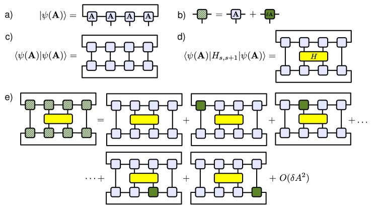
Hence the first term in (3) is proportional to the gradient of the energy density $\rho_{E}(\mathbf{a})=\langle H_{s,s+1}\rangle_{\mathbf{A}}$, $\forall s\in[1,N]$ (see figure 2d). Second, we can obtain gradients such as the ones occurring in (3) numerically at a given point $\mathbf{a}$ by expanding the differentiated quantity in powers of $\delta\mathbf{a}$ and computing the coefficient of the linear term. Thus the derivative in the first term is obtained via

$$\rho_{E}(\mathbf{a}+\delta\mathbf{a})=\rho_{E}(\mathbf{a})+\delta\mathbf{a}\bigl{[}\nabla_{\mathbf{a}^{\prime}}\rho_{E}(\mathbf{a}^{\prime})\bigr{]}_{\mathbf{a}^{\prime}=\mathbf{a}}+O(\delta\mathbf{a}^{2})$$ (4)

and the one in the second via

$$\braket{\psi(\mathbf{a}+\delta\mathbf{a})}{\psi(\mathbf{a}+\delta\mathbf{a})}=\braket{\psi(\mathbf{a})}{\psi(\mathbf{a})}+\delta\mathbf{a}\bigl{[}\nabla_{\mathbf{a}^{\prime}}\braket{\psi(\mathbf{a}^{\prime})}{\psi(\mathbf{a}^{\prime})}\bigr{]}_{\mathbf{a}^{\prime}=\mathbf{a}}+O(\delta\mathbf{a}^{2})\,\,\,.$$ (5)

Let us first consider (4). This can can be computed explicitly by taking a sum of completely contracted tensor networks (see figure 2e). Let $H_{eff}(\mathbf{A})$ denote the object that is obtained by removing the tensor $\delta\mathbf{A}$ from each term of $\rho_{E}(\mathbf{a}+\delta\mathbf{a})$ that is linear in $\delta\mathbf{a}$ (see figure 3). This is a tensor with three indices, that reshaped in vector form, yields the desired derivative $\nabla\rho_{E}(\mathbf{a})=\mbox{vec}(H_{eff}(\mathbf{A}))$. The computational cost for the exact contraction of the tensor networks in $H_{eff}(\mathbf{A})$ scales as $O(ND^{5})$ Verstraete et al. (2004). We will give below a prescription of how this can be improved to $O(mnD^{3})+O(n^{2}D^{3})$ for chains of arbitrary lengths. Furthermore we will show how to choose the smallest possible parameters $m$ and $n$ such that no loss in precision occurs and why the scaling reduces to $O(mD^{3})+O(nD^{3})$ in the case of very long chains.

Figure 3: (Color online). Graphical representation of the tensor $H_{eff}(\mathbf{A})$ and $N_{eff}(\mathbf{A})$.

The other piece that is necessary for the computation of $\nabla E(\mathbf{a})$, is the derivative occurring in the second term of (3); this term can be obtained in a very similar way (see figure 3). We will use the notation $N_{eff}(\mathbf{A})$ for the object defined by $\nabla\braket{\psi(\mathbf{a})}{\psi(\mathbf{a})}=:\mbox{vec}(N_{eff}(\mathbf{A}))$. Due to the simpler structure of the tensor network the computational cost here will scale as $O(nD^{3})$ for arbitrary chains and as $O(D^{3})$ for very long chains.

Now let us introduce the following convention for denoting incomplete tensor networks where merely one of the MPS tensors is missing: $\langle O\rangle_{\mathbf{A}}^{[\overline{s}]}$ shall henceforth denote the expectation value of the operator $O$ with respect to the TI MPS defined by the tensor ${\mathbf{A}}$, where one tensor ${\mathbf{A}}$ has removed been removed from $\ket{\psi({\mathbf{A}})}$ at site $s$. Following this definition, the first term in the graphical representation of $H_{eff}({\mathbf{A}})$ (see figure 3) reads $\langle H_{2,3}\rangle_{\mathbf{A}}^{[\overline{1}]}$. If a tensor has been removed from $\bra{\psi({\mathbf{A}})}$ at site $s$, we will denote this by underlining the site index, thus we write $\langle O\rangle_{\mathbf{A}}^{[\underline{s}]}$. Using this convention we can write $H_{eff}({\mathbf{A}})$ as

$$H_{eff}({\mathbf{A}})=\sum_{s=1}^{N}\Big{(}\langle H_{1,2}\rangle^{[\overline{s}]}_{\mathbf{A}}+\langle H_{1,2}\rangle^{[\underline{s}]}_{\mathbf{A}}\Big{)}\,\,\,.$$ (6)

For real Hamiltonians and real MPS this reduces of course to

$$H_{eff}({\mathbf{A}})=2\sum_{s=1}^{N}\langle H_{1,2}\rangle^{[\overline{s}]}_{\mathbf{A}}\,\,\,.$$ (7)

Similar considerations hold for $N_{eff}({\mathbf{A}})$. Thus, using $I$ to denote the identity operator, we can rewrite the gradient of the energy (3) as

$$\nabla E({\mathbf{a}})=\frac{NH_{eff}({\mathbf{A}})}{\braket{\psi({\mathbf{A}})}{\psi({\mathbf{A}})}}-\frac{N\rho_{E}({\mathbf{a}})N_{eff}({\mathbf{A}})}{\braket{\psi({\mathbf{A}})}{\psi({\mathbf{A}})}^{2}}=2N\sum_{s=1}^{N}\Big{(}\frac{\langle H_{1,2}\rangle^{[\overline{s}]}_{\mathbf{A}}}{\langle I\rangle_{\mathbf{A}}}-\frac{\langle H_{1,2}\rangle_{\mathbf{A}}\langle I\rangle^{[\overline{s}]}_{\mathbf{A}}}{\langle I\rangle_{\mathbf{A}}^{2}}\Big{)}\,\,\,.$$ (8)

In the last part of this section we will briefly sketch how a gradient based procedure can be employed to find ground states of PBC chains if one is dealing with complex Hamiltonians and thereby complex MPS. One possibility is to use a gradient based algorithm that converges to a minimum of the real-valued function $E:\mathbb{C}^{n}\rightarrow\mathbb{R}$ within the complex manifold ($n$ stands here for the number of independent complex parameters in the MPS). It can be shown that in this case one obtains the same expression (8) for the gradient of the energy albeit the individual terms are now complex valued vectors. However, since standard library routines for gradient based search cannot minimize over complex manifolds, let us mention the second possibility just for the sake of completeness. Due to ${\mathbf{a}}={\mathbf{x}}+i{\mathbf{y}}$ with ${\mathbf{x}},{\mathbf{y}}\in\mathbb{R}^{n}$, one can treat the energy as an analytic function over a real manifold with twice as many degrees of freedom, i.e. $E:\mathbb{R}^{2n}\rightarrow\mathbb{R}$. Similar considerations to the ones leading to (8) yield then for the gradient

$$\begin{split}\nabla_{{\mathbf{x}}}E({\mathbf{x}},{\mathbf{y}})&=\phantom{-}2N\sum_{s=1}^{N}\Big{(}\frac{\operatorname{Re}\langle H_{1,2}\rangle^{[\overline{s}]}_{\mathbf{A}}}{\langle I\rangle_{\mathbf{A}}}-\frac{\langle H_{1,2}\rangle_{\mathbf{A}}\operatorname{Re}\langle I\rangle^{[\overline{s}]}_{\mathbf{A}}}{\langle I\rangle_{\mathbf{A}}^{2}}\Big{)}\\ \nabla_{{\mathbf{y}}}E({\mathbf{x}},{\mathbf{y}})&=-2N\sum_{s=1}^{N}\Big{(}\frac{\operatorname{Im}\langle H_{1,2}\rangle^{[\overline{s}]}_{\mathbf{A}}}{\langle I\rangle_{\mathbf{A}}}-\frac{\langle H_{1,2}\rangle_{\mathbf{A}}\operatorname{Im}\langle I\rangle^{[\overline{s}]}_{\mathbf{A}}}{\langle I\rangle_{\mathbf{A}}^{2}}\Big{)}\,\,\,.\end{split}$$ (9)

III.1 Computation of $H_{eff}({\mathbf{A}})$

We introduce now a shorthand notation for the building blocks of $H_{eff}(\mathbf{A})$ that will allow us to express it in a very compact way. From the graphical representation (see figure 4) it should be obvious what the objects $H_{AA}^{AA}$, $H_{AA}^{\phantom{A}A}$, $H_{AA}^{A\phantom{A}}$, $T=T_{A}^{A}$ and $T_{A}$ mean; note that $T$ denotes the MPS transfer matrix that has been repeatedly mentioned in the previous sections. For the sake of completeness we also give the definition of the tensor $H_{AA}^{AA}$ explicitly in terms of its components:

Figure 4: (Color online). Graphical representation of $H_{AA}^{AA}$, $H_{AA}^{\hskip 6.54413ptA}$, $H_{AA}^{A}$, $T=T_{A}^{A}$ and $T_{A}$.

$$(H_{AA}^{AA})^{\alpha\phantom{\alpha^{\prime}}\gamma}_{\phantom{\alpha}\alpha^{\prime}\phantom{\gamma}\gamma^{\prime}}=A_{i\phantom{\alpha}\beta}^{\phantom{i}\alpha}A_{j\phantom{\beta}\gamma}^{\phantom{i}\beta}(H_{s,s+1})^{ij}_{\phantom{ij}i^{\prime}j^{\prime}}A_{\phantom{i^{\prime}}\alpha^{\prime}}^{i^{\prime}\phantom{\alpha^{\prime}}\beta^{\prime}}A_{\phantom{j^{\prime}}\beta^{\prime}}^{j^{\prime}\phantom{\beta^{\prime}}\gamma^{\prime}}\,\,\,.$$ (10)

Here we have used greek letters to label the virtual bonds, latin ones for the physical bonds and Einstein summation convention to denote contracted indices. If one combines the left-hand side indices $\alpha$ and $\alpha^{\prime}$ into one big index and does the same for the right-hand side indices $\gamma$ and $\gamma^{\prime}$, it is clear that $H_{AA}^{AA}$ represents a $D^{2}\times D^{2}$-matrix. The other objects defined in figure 4 have similar explicit definitions. $H_{eff}({\mathbf{A}})$ now reads

$$H_{eff}({\mathbf{A}})=2\cdot\mbox{Tr}^{*}\Big{[}H_{AA}^{\phantom{A}A}T^{N-2}+H_{AA}^{A\phantom{A}}T^{N-2}+\sum_{s=0}^{N-3}H_{AA}^{AA}T^{s}T_{A}T^{N-3-s}\Big{]}$$ (11)

where $\mbox{Tr}^{*}[\dots]$ indicates that the trace is taken only with respect to the matrix multiplication of the ”outer” indices of the ”big” $D^{2}\times D^{2}$-matrices. These ”big” matrices may have internal open indices that survive the $\mbox{Tr}^{*}[\dots]$-operation and make sure that $H_{eff}({\mathbf{A}})$ is left with its tensor structure s.t. it can be later reexpressed as a vector.

The computation of (11) is the bottleneck of our method. If we would compute it by straightforward matrix multiplication, even using the sparseness, the computational cost would scale as $O(ND^{5})$. In order to improve this scaling, the crucial point is to realize that for large $N$ most terms in (11) will contain high powers of $T$ which means that they can be very well approximated within the subspace spanned by the dominant eigenvectors of $T$. This can be easily seen if we write such factors in their eigenbasis

$$T^{s}=\sum_{\alpha=1}^{D^{2}}\lambda_{\alpha}^{s}\ket{\lambda_{\alpha}}\bra{\lambda_{\alpha}}=\lambda_{1}^{s}\bigg{[}\ket{\lambda_{1}}\bra{\lambda_{1}}+\sum_{\alpha=2}^{D^{2}}\bigg{(}\frac{\lambda_{\alpha}}{\lambda_{1}}\bigg{)}^{s}\ket{\lambda_{\alpha}}\bra{\lambda_{\alpha}}\bigg{]}$$ (12)

where $\lvert\lambda_{1}\rvert\geq\lvert\lambda_{2}\rvert\dots\geq\lvert\lambda_{D^{2}}\rvert$. Obviously the subspace corresponding to the small magnitude eigenvalues is suppressed exponentially with $s$ and thus can be neglected for powers $s$ that are large enough (e.g. for $s=20$ and $\lvert\frac{\lambda_{\alpha}}{\lambda_{1}}\rvert\approx 0.1$, $\lvert\frac{\lambda_{\alpha}}{\lambda_{1}}\rvert^{s}\approx 10^{-20}<10^{-16}$ which is the machine precision of double precision floating point numbers). In these cases it is perfectly fine to restrict ourselves to the subspace spanned by say $n$ dominant eigenvectors, with the parameter $n$ yet to be determined. In fact, we will perform the entire computation a few times, starting with a rather small $n$ and increasing it until the result does not improve any more. When this happens, we know that we have found the optimal $n$ beyond which, when all other parameters are fixed, the precision does not get any better. Thus we will approximate large powers of the transfer matrix as

$$T^{s}\approx\sum_{\alpha=1}^{n}\lambda_{\alpha}^{s}\ket{\lambda_{\alpha}}\bra{\lambda_{\alpha}}\,\,\,.$$ (13)

At this point we must remark that this approximation only works if the moduli of the transfer matrix eigenvalues $\lvert\lambda_{\alpha}\rvert$ are not concentrated around a certain point (i.e. $T$ is not approximately proportional to unity). In that case, any increment of $n$ will improve the precision and we will end up with very bad overall scaling . For models where this behaviour occurs the algorithm presented here may be worse than contracting the tensor networks explicitly, where the scaling is $O(ND^{5})$. In these cases the chain length $N$ ultimately decides which method is preferable. Fortunately for the models treated by us, this undesirable behaviour does not occur and we end up with relatively small $n$ beyond which the precision does not improve any more.

Let us now return to (11). There are two different types of terms which must be treated differently. The first and the second term under our somewhat unorthodoxly defined trace can be considered as ”easy”. They are approximated by

$$\langle H_{1,2}\rangle^{[\overline{1}]}_{\mathbf{A}}=\mbox{Tr}^{*}\Big{[}H_{AA}^{\phantom{A}A}T^{N-2}\Big{]}\approx\sum_{\alpha=1}^{n}\bra{\lambda_{\alpha}}H_{AA}^{\phantom{A}A}\ket{\lambda_{\alpha}}\lambda_{\alpha}^{N-2}$$ (14)

which is computed within $O(nD^{3})$ operations. This is because each contraction $\bra{\lambda_{\alpha}}H_{AA}^{\phantom{A}A}\ket{\lambda_{\alpha}}$ can be performed with cost $O(D^{3})$ and this has to be done $n$ times.

The computationally more expensive terms are the ones under the sum over $s$, where two different powers of $T$ are involved. We will call these terms ”hard”. They are approximated by

$$\langle H_{1,2}\rangle^{[\overline{3+s}]}_{\mathbf{A}}=\mbox{Tr}^{*}\Big{[}H_{AA}^{AA}T^{s}T_{A}T^{N-3-s}\Big{]}\approx\sum_{\alpha,\beta=1}^{n}\bra{\lambda_{\beta}}H_{AA}^{AA}\ket{\lambda_{\alpha}}\bra{\lambda_{\alpha}}T_{A}\ket{\lambda_{\beta}}\lambda_{\alpha}^{s}\lambda_{\beta}^{N-3-s}\,\,\,.$$ (15)

Here we must remark two things: i) it is not necessary to let the second index $\beta$ run over the same range as $\alpha$. It would be possible to choose as an upper bound a further parameter $n^{\prime}$ and also vary this one until the precision does not improve any more. However, since expression (15) has obviously left-right symmetry, it is sensible to assume that the optimal result would yield $n=n^{\prime}$. Even if this would not be the case, due to the fact that we scan along $n$, convergence will be reached only for some $n_{\textrm{optimal}}\geq\sup\{n,n^{\prime}\}$, so we will find the lowest achievable energy anyway; ii) for very small or very large $s$ either the left or the right transfer matrix segments in (15) can not be well approximated by a little number of eigenvalues $n$ since the lower $\lambda_{\alpha}$ are not sufficiently suppressed by the small exponent. In the worst case we would have to take all $D^{2}$ eigenvalues into account, which dramatically increases the computational cost. In order to solve this issue we will compute these terms by exact contraction of segments of length $m$, which introduces this further parameter into our algorithm. This will be explained in more detail further below. For the moment let us note that depending on the magnitude of $s$, we can further separate the sum in (11) over the ”hard” terms into

$$\sum_{s=0}^{N-3}\equiv\sum_{s=0}^{m-1}+\sum_{s=m}^{N-3-m}+\sum_{s=N-2-m}^{N-3}\,\,\,.$$ (16)

We call the terms over which the second sum is taken ”medium-$s$” terms and will treat them differently from the ”extremal-$s$” terms that appear in the first respectively third sum. Thus $H_{eff}({\mathbf{A}})$ can be divided into

$$H_{eff}({\mathbf{A}})=2\cdot\bigg{(}H_{eff}^{easy}({\mathbf{A}})+H_{eff}^{hard,extr}({\mathbf{A}})+H_{eff}^{hard,med}({\mathbf{A}})\bigg{)}\,\,\,.$$ (17)

III.1.1 Computation of ”extremal-$s$” terms

In this section we treat the terms with small respectively large $s$. The first thing to remark is that for large $N$, if $T^{s}$ can not be well approximated within some low-dimensional subspace because $s$ is too small, it is very likely that for $T^{N-3-s}$ the approximation will work due to $N-3-s\gg s$. The same observation holds in the other direction if $s$ is too large. Secondly, depending on the MPS bond dimension $D$ and the ammount of entanglement present in the MPS (i.e. depending on the model one is treating), there is a certain $m$ above which $T^{s}$ with $s\geq m$ can be faithfully approximated within the $n<D^{2}$-dimensional subspace spanned by $n$ dominant eigenvectors. As we don’t know anything about $m$ a priori, we introduce it as a further parameter into our algorithm. We will scan $m$ within its range $[1,1/2(N-2)]$ and in the end we will obtain some optimal pair $(m,n)$. The reason why $m$ does not go all the way up to $N-3$ is that in order for our algorithm to scale effectively as $D^{3}$, we must employ the dominant eigenvector approximation on the other half of the chain. Without it we would get the undesirable scaling $O(ND^{5})$. The contraction (see figure 5) we must perform for each term with small $s$ thus reads

$$\langle H_{1,2}\rangle^{[\overline{3+s}]}_{\mathbf{A}}=\mbox{Tr}^{*}\Big{[}H_{AA}^{AA}T^{s}T_{A}T^{N-3-s}\Big{]}\approx\sum_{\alpha=1}^{n}\bra{\lambda_{\alpha}}H_{AA}^{AA}T^{s}T_{A}\ket{\lambda_{\alpha}}\lambda_{\alpha}^{N-3-s}\,\,\,,\,\,\,\forall s<m$$ (18)

and can be done with computational cost $O(nD^{3})$ using a sparse matrix contraction scheme. As we have to repeat this procedure $m$ times, the total cost scales as $O(mnD^{3})$.

Figure 5: (Color online). Graphical representation of a term with small $s$ and its approximation within the subspace spanned by $n$ dominant eigenvectors of $T$.

The large $s$ terms (i.e. when $N-3-m<s\leq N-3$) can be easily obtained by making use of the left-right symmetry of the tensor network around the point with $s=(N-2)/2$. The sum over all these $s$ turns out to be related to the sum over the small $s$ terms by taking the transpose with respect to the open virtual bond indices at the empty site where $T_{A}$ sits. Thus the computational cost remains unchanged $O(mnD^{3})$.

III.1.2 Computation of ”medium-$s$” terms

For terms where $s$ is neither too small nor too large, both powers of the transfer matrix (i.e. $T^{s}$ and $T^{N-3-s}$) can be well approximated whithin the subspace spanned by $n$ dominant eigenvectors. The good news is that in this case the sum over $s$ can be performed analitically in contrast to the ”extremal-$s$” case where we had to compute each of the $m$ terms separately. However, there is also bad news, namely that we now have an additional sum over the eigenvalue index stemming from the approximation of $T^{N-3-s}$. Explicitly the sum over all ”medium-$s$” reads

$$\begin{split}H_{eff}^{hard,med}({\mathbf{A}})&=\mbox{Tr}^{*}\Big{[}\sum_{s=m}^{N-3-m}H_{AA}^{AA}T^{s}T_{A}T^{N-3-s}\Big{]}\\ &\approx\mbox{Tr}^{*}\Big{[}\sum_{s=0}^{N-3-2m}\sum_{\alpha,\beta=1}^{n}H_{AA}^{AA}T^{m}\ket{\lambda_{\alpha}}\lambda_{\alpha}^{s}\bra{\lambda_{\alpha}}T_{A}\ket{\lambda_{\beta}}\lambda_{\beta}^{N-3-2m-s}\bra{\lambda_{\beta}}T^{m}\Big{]}\\ &=\sum_{\alpha,\beta=1}^{n}\bra{\lambda_{\beta}}H_{AA}^{AA}\ket{\lambda_{\alpha}}\bra{\lambda_{\alpha}}T_{A}\ket{\lambda_{\beta}}\lambda_{\alpha}^{m}\lambda_{\beta}^{m}\frac{\lambda_{\beta}^{N-2-2m}-\lambda_{\alpha}^{N-2-2m}}{\lambda_{\beta}-\lambda_{\alpha}}\,\,\,.\end{split}$$ (19)

In the first step we have shifted the summation variable $s$ and have written the matrices $T$ in their eigenbasis. To arrive from the second to the third line we have used the cyclic property of the trace to write the entire expression as a sum over products of scalars (actually the factor containing $T_{A}$ is only a scalar with respect to our specially defined trace since it contains internal free indices). Furthermore we have performed the $s$-sum straightforwardly.

The computational cost scales here as $O(n^{2}D^{3})$. This is because we have two sums going from $1$ to $n$ over terms that are contracted within $O(D^{3})$ operations.

III.2 Computation of $N_{eff}({\mathbf{A}})$

Our prescription for the computation of $N_{eff}({\mathbf{A}})$ is also based on the observation that big powers of the transfer matrix $T$ can be very well approximated within the subspace spanned by the dominant eigenvectors. However here things are much easier than for $H_{eff}({\mathbf{A}})$. This is because the translational invariance is not broken by the 2-site Hamiltonian (see figure 3) and we can write

$$N_{eff}({\mathbf{A}})=2N\cdot\langle I\rangle^{[\overline{1}]}_{\mathbf{A}}\,\,\,.$$ (20)

Similarly to $\langle H_{1,2}\rangle^{[\overline{1}]}_{\mathbf{A}}$ in (14), $\langle I\rangle^{[\overline{1}]}_{\mathbf{A}}$ is approximated by

$$\langle I\rangle^{[\overline{1}]}_{\mathbf{A}}=\mbox{Tr}^{*}\Big{[}T_{A}T^{N-1}\Big{]}\approx\sum_{\alpha=1}^{n}\bra{\lambda_{\alpha}}T_{A}\ket{\lambda_{\alpha}}\lambda_{\alpha}^{N-1}$$ (21)

which is computed within $O(nD^{3})$ operations.

III.3 Overall scaling of the computational cost

We have seen that the gradients in (3) can be obtained within $O(mnD^{3})+O(n^{2}D^{3})$ respectively $O(nD^{3})$ operations if our approximation of large powers of the transfer matrix is justified. It is easy to check that the scalar expectation values in (3) can be obtained in an analogue yet simpler way. The fact that there are no vacant sites in the corresponding tensor networks enables us to use everywhere a method identical to the one used for $N_{eff}({\mathbf{A}})$. Thus the computational cost for our algorithm scales as its most expensive part, namely as $O(mnD^{3})+O(n^{2}D^{3})$.

It is also not difficult to check that for very large chains (i.e. either when $N\gg\xi$ for non-critical systems or $N\gg\tilde{\xi}_{D}$ for critical ones, where $\tilde{\xi}_{D}$ is the effective correlation length induced by finite $D$) this scaling can be improved. First recall that we had in every tensor network at least one portion of the chain expressed as a power of $T$ that we approximated using its dominant eigenvectors. Now, for any bond dimension $D$ there exists an $N$ above which all approximated portions are long enough s.t. all eigenvalues except the largest one are suppressed by the very large exponent. In this case the overall scaling is $O(mD^{3})+O(nD^{3})$. Note that in the scaling for the ”extremal-s” terms we can not get rid of $m$ because there will always be short portions between the $H_{1,2}$ and the vacant site, that must be contracted exactly. Similarly, for the ”medium-s” terms (19) only the combinations of $\lambda_{\alpha}^{m}\lambda_{\beta}^{m}$ where both $\alpha$ and $\beta$ are large will be negligible. Factors like $\lambda_{1}^{m}\lambda_{\beta}^{m}$ must usually always be taken into account. In any case, the ultimate check whether our approximations are justified must be done in the simulations, where one must verify if there exists an $n$ beyond which the ground state energy does not decrease.

We would like to compare our scaling of the computational cost to the one of Pippan et al. (2010) once again. Note that expressed in the terms used in this work, the scaling from Ref. Pippan et al. (2010) is $O(NnD^{3})$. On one hand, as previously mentioned, our TI algorithm yields an improvement of one factor $N$. On the other hand there is an additional factor $n$ that appears in our scaling. This is due to the fact that we compute the gradient of the energy explicitly. It is easy to see that the computational cost for the evaluation of the energy itself is $O(nD^{3})$. However if we would restrict ourselves to evaluations of the energy only, we would have to use something like a downhill simplex method as the outer function that scans the MPS manifold for the energy minimum. In this case the outer function would call the energy evaluator a huge number of times, thereby yielding the overall cost much higher than one factor of $n$ that we must pay when computing the gradient.

IV Numerical results

We have studied both critical and non-critical nearest neighbour interaction spin models. The first one is the Quantum Ising model for spins-$1/2$

$$H_{IS}=-\sum_{<ij>}Z_{i}Z_{j}-B\sum_{i}X_{i}$$ (22)

which we have simulated at its critical point $B=1$. The second one is the antiferromagnetic Heisenberg model

$$H_{HB}=\frac{1}{2}\sum_{<ij>}(X_{i}X_{j}+Y_{i}Y_{j}+Z_{i}Z_{j})\,\,\,.$$ (23)

This model is critical for spin-$1/2$ chains but non-critical for spin-$1$ chains. We have studied both cases. Note that (23) is not very well suited for the description with 1-site TI MPS due to its antiferromagnetic character. In order to cure this problem we apply in the case of the spin-$1/2$ chain a global unitary consisting of Pauli-$Y$ matrices on each second site . This leaves the spectrum unchanged and after we have found the 1-site TI MPS for the ground state, we can recover the one for the unchanged Hamiltonian by a new application of the global unitary. The resulting MPS is then of course 2-site TI. The rotated Heisenberg Hamiltonian reads

$$H_{HB}=\frac{1}{2}\sum_{<ij>}(-X_{i}X_{j}+Y_{i}Y_{j}-Z_{i}Z_{j})\,\,\,.$$ (24)

IV.1 Critical systems

Figure 6: (Color online). Critical Quantum Ising chain with $N=100$: Relative precision of the MPS ground state energy as compared to the analytical result as a function of the parameters $(m,n)$ for $D=16$ (left) and $D=32$ (right).

Figure 7: (Color online). Critical Heisenberg chain with $N=100$: Relative precision of the MPS ground state energy as compared to the analytical result as a function of the parameters $(m,n)$ for $D=16$ (left) and $D=32$ (right).

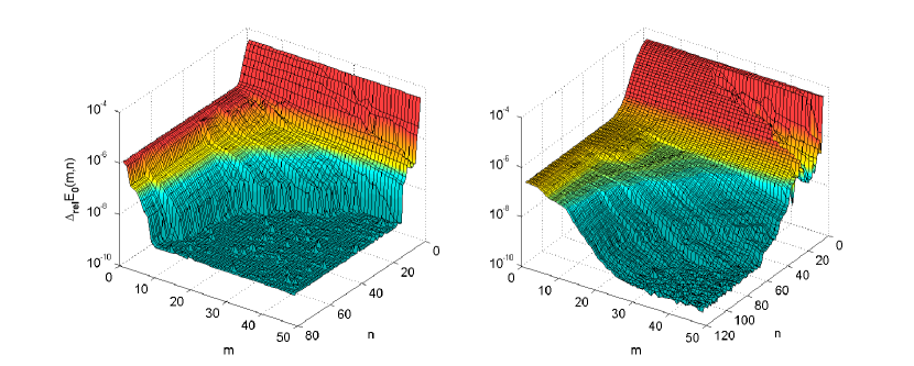
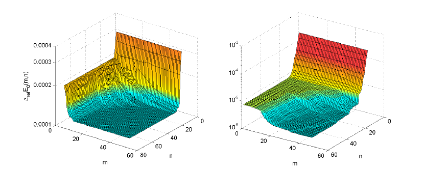
Let us illustrate the strategy for the scan of the parameter space spanned by $\{m,n\}$ on the basis of results obtained for small critical chains of $100$ and $400$ sites. Figure 6 and figure 7 show the relative precision $\Delta_{rel}E_{0}(m,n)=(E_{0}^{exact}-E_{0}^{MPS}(m,n))/E_{0}^{exact}$ of the MPS ground state energy compared to the exact solution as a function of the algorithm parameters $m$ and $n$ for the Quantum Ising respectively Heisenberg chain. The first observation is that there exist $m_{max}$ and $n_{max}$ s.t. for all $m\geq m_{max}$, $n\geq n_{max}$ the precision does not improve any more. In the featured plots the plateau $\mathcal{P}$ with minimal energy is reached within the plot range. The optimal point $\{m_{opt},n_{opt}\}$ is then the point of $\mathcal{P}$ that minimizes the scaling of the computational cost $O(mnD^{3})+O(n^{2}D^{3})$ i.e. $\{m_{opt},n_{opt}\}=\min|_{\{m,n\}\in\mathcal{P}}(mn+n^{2})$. Clearly, the optimal parameters $m_{opt}$ and $n_{opt}$ will be different for different models and different values of the chain length $N$ and the MPS bond dimension $D$.

The plots reveal a further detail: if we are not very pedantic about the optimal $\{m,n\}$-pair, it is not necessary to scan the entire plane, which is computationally very expensive. If we are willing to settle for any pair $\{m,n\}$ that yields maximal precision, we can scan along any line $n=km$ and we can be sure that at some point we will hit $\mathcal{P}$. This pair is quasi-optimal in the sense that we have found the optimal $n$ for the corresponding $m$ and vice versa. This is due to the fact that for any point of $\mathcal{P}$, especially for its boundary, walking along lines with increasing $m$ or $n$ does not take us out of $\mathcal{P}$. As one can see in figure 6 and 7, $\mathcal{P}$ is roughly symmetric in $m$ and $n$, so a sensible line to scan along is given by $n=m$ . As we have mentioned before, our algorithm allows us to increase $m$ only up to $(N-2)/2$. If until then, the results obtained along $n=m$ have not converged yet, we must continue the scan along the line given by the constant maximal $m$ towards larger $n$.

Figure 8: (Color online). Critical Quantum Ising chain with $N=100$ (left) and $N=400$ (right): Relative precision of the MPS ground state energy as a function of the parameter $n$ for different bond dimensions $D$. The scan has been performed along the line $m=5n$ up to the maximal value of $m$ and then along the line with constant $m=(N-2)/2$.

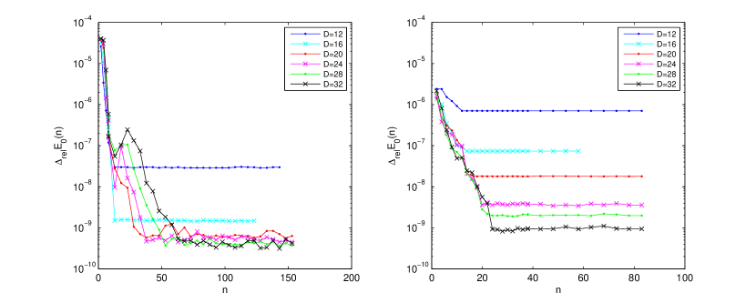
The relative precision of the MPS ground state energy for such line scans is plotted in figure 8. We notice that with increasing $D$ the maximally reachable precision gets better in concordance to what one would expect. The fact that $m_{opt}$ and $n_{opt}$ increase with $D$ is also intuitive. What is a bit surprising is that for small $n$ the results obtained for small bond dimensions are either similar or even better than the ones obtained for higher bond dimensions. This means that if one is not willing to go to larger values of $n$, there is no point in increasing $D$!

Another interesting point is that for fixed $D$, as we increase $N$, the plateau $\mathcal{P}$ is reached sooner and sooner (i.e. for smaller values of $n$ and implicitly of $m$). This behaviour is due to the fact that with increasing $N$ the weight that we loose in our contracted tensor network by choosing $n<D^{2}$ becomes negligible at smaller $n$.

IV.2 Observables - energy and correlation functions

Figure 9: (Color online). Critical Quantum Ising model: relative precision of the MPS ground state energy for different $N$ as a function of $D$.

Figure 10: (Color online). Critical Heisenberg model: relative precision of the MPS ground state energy for different $N$ as a function of $D$.

As the computational cost of our algorithm actually decreases if we increase the number of sites $N$ while keeping $D$ constant, we can investigate PBC chains of arbitrary size . Figure 9 and figure 10 show the relative precision of the ground state energy for the critical Quantum Ising respectively Heisenberg model as a function of the MPS bond dimension $D$. We can see that generally the relative error is decreasing as a polynomial of $D$ i.e. $\Delta_{rel}E_{0}(D)\propto D^{-\mu}$. We have fitted straight lines through the reliable data of the $N=100$ and $N=5000$ plots and have obtained for the exponent $\mu$ the values $7.84$ and $3.21$ ($6.12$ and $2.52$) for the critical Quantum Ising (Heisenberg) model. In the central plots (i.e. $N=500$ and $N=1000$) one can distinguish between two regions where the relative precision is decaying polynomially with the exponents obtained from the outer plots (i.e. $N=100$ and $N=5000$). We have emphasized this by drawing dashed lines through the data points in the central plots. Note that the dashed lines are not fitted, they have merely the same slope as the full lines in the outer plots. This behaviour can be best understood if one looks at correlation functions.

Figure 11: (Color online). Correlation functions for a critical Quantum Ising chain with $N=500$. Left: order parameter correlator $\Gamma^{ZZ}(\Delta r)$ and as inset the half-chain correlator as a function of $D$. Right: correlator $\Gamma^{XX}(\Delta r)$ and as inset the half-chain correlator as a function of $D$.

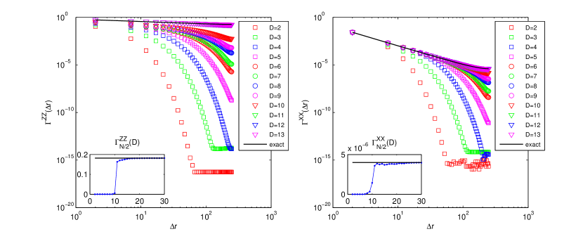
Let us first consider the critical Quantum Ising model. In figure 11 we have plotted the $ZZ$ and the $XX$ correlation functions $\Gamma^{ZZ}(\Delta r)$ and $\Gamma^{XX}(\Delta r)$ in the MPS ground state of a chain with $N=500$ sites. The solid line represents the exact solution obtained by applying the programme of Lieb et al. (1961) to the Quantum Ising model with PBC. One can clearly see that with increasing $D$ the MPS correlations become more and more accurate, just as one would expect. Note that we have only plotted the correlation functions for separations $\Delta r\leq N/2$. This is because due to the periodic boundary conditions $\Gamma(\Delta r)$ is symmetric around $\Delta r=N/2$ . We would like to point out that while the exact $\Gamma(\Delta r)$ is linear for small $\Delta r$ thus implying polynomial decay of correlations in that regime, it flattens out towards $\Delta r\approx N/2$. This behaviour is consistent with the physical requirement that the correlation function is smooth at $\Delta r=N/2$. The insets show the value of the half-chain correlators $\Gamma_{N/2}(D):=\Gamma(\Delta r=N/2,D)$ as a function of $D$. One can clearly see a jump in $\Gamma_{N/2}(D)$ at some $D^{\prime}$. This means that in this model, if one wants to obtain good approximations for long range correlations in the ground state, one must use MPS with bond dimension $D\geq D^{\prime}(N)$. Note that the jump in the inset of figure 11 occurs roughly in the same region as the change of the slope in the second plot of figure 9. This allows us to understand why in figure 9 the slope for large $D$ is steeper than the one for small $D$: if $D$ is not large enough such that correlations are faithfully reproduced throughout the entire chain, this represents a further source of error besides the inherent error of MPS with non-exponential bond dimension (i.e. $D\ll d^{N/2}$).

Figure 12: (Color online). Absolute value of the correlation functions for a critical Heisenberg chain with $N=500$. Left: correlator $\Gamma^{ZZ}(\Delta r)$ and as inset the half-chain correlator as a function of $D$. Right: correlator $\Gamma^{XX}(\Delta r)$ and as inset the half-chain correlator as a function of $D$.

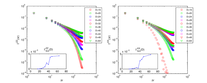
The absolute value of the correlation functions for the critical Heisenberg chain with $N=500$ sites can be found in figure 12. Note that these plots only contain the MPS data since we do not have analytical expressions for the long range correlations. Qualitatively figure 12 shows the same behaviour as figure 11. Quantitatively we can see that correlation functions converge at much larger $D$ than in the case of the critical Quantum Ising model, which is exactly what we would expect. The half-chain correlators $\Gamma_{N/2}(D)$ exhibit a more or less continuous transition to the region where correlations are faithfully reproduced.

Figure 13: (Color online). Relative precision of correlation functions in the MPS ground state of the Quantum Ising model with $N=500$. Left: error of the order parameter correlation function $\Gamma^{ZZ}(\Delta r)$ for several different $D$ in the high precision regime. Right: relative precision of the half-chain correlators $\Gamma_{N/2}^{ZZ}$ and $\Gamma_{N/2}^{XX}$ as a function of the MPS bond dimension $D$.

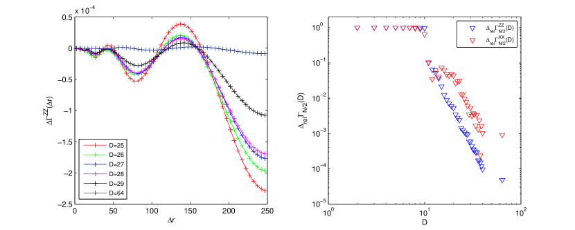
We would like to make an interesting final remark regarding the error in the correlation functions as a function of $\Delta r$. In the left part of figure 13 we have plotted $\Gamma^{ZZ}_{MPS}(\Delta r)-\Gamma^{ZZ}_{exact}(\Delta r)$ for different $D$ in the regime where the half-chain correlators have well converged (i.e. $D>25$). The surprising thing is that the error does not grow monotonically as a function of $\Delta r$ as one would expect, but that it rather oscillates around zero. Nevertheless the amplitude of the oscillations is growing monotonically with $\Delta r$. The right part of figure 13 reveals that similary to the relative error of the ground state energy, the relative error of the half-chain correlators $\Delta_{rel}\Gamma_{N/2}(D)$ obeys power-law decay as a function of $D$ in the large $D$ regime.

Our numerical analysis thus indicates that for each $N$ there is a minimum value of $D=D^{\prime}(N)$ such that correlations throughout the entire chain are properly captured. As investigated in Pirvu et al. (2010), for critical systems this minimum value of $D^{\prime}(N)$ is seen to be given by a small power of $N$ that depends on the universality class of the model. This dependence will allow us in Pirvu et al. (2010) to characterize the cost of the algorithm presented in this work as a power of $N$. For the moment we will settle for a scaling of the overall computational cost of $O(g(D,\xi/N)D^{3})$ where $g(D,\xi/N)$ will be seen to become trivial only for non-critical systems.

IV.3 Non-critical systems

Figure 14: (Color online). Spin-$1$ Heisenberg chain with $N=100$: Relative precision of the MPS ground state energy as compared to the best numerical approximation as a function of the parameters $(m,n)$ for $D=16$ (left) and $D=100$ (right).

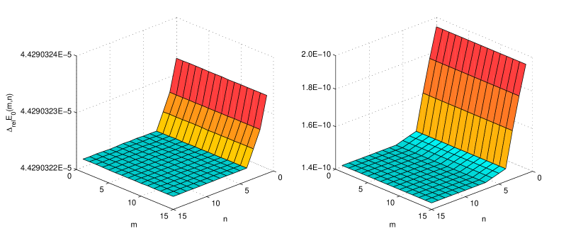
We have seen that for critical systems it is quite involved to predict the computational cost of MPS algorithms that find the optimal approximation of the ground state within the manifold defined by MPS with fixed bond dimension $D$. This turns out to be much easier for non-critical systems where the correlation length $\xi$ is much smaller than the chain length $N$. We have studied the spin-$1$ Heisenberg chain as the prototype of a non-critical quantum spin chain in order to be able to compare our results with the ones presented in Ref. Pippan et al. (2010). As pictured in figure 14, for $N=100$ and $D$ that is not too big, $n=4$ is sufficient in order to obtain the optimal MPS approximation to the ground state. This is in agreement with the predictions of Ref. Pippan et al. (2010). However for $D$ as big as $100$, we would have to choose $n=7$ if we are not willing to loose any precision. This indicates a dependence of $n$ on $D$ which is much weaker than in the case of critical systems. Since due to finite computer memory we cannot increase $D$ arbitrarily, it is safe to say that for systems where $\xi\ll N$, $n$ is given by a small constant. This is exactly what happens for a spin-$1$ Heisenberg chain with $100$ sites since as shown in Ref. White and Huse (1993) the correlation length is roughly $\xi\approx 6$ s.t. $\xi\ll N$. It is obvious from figure 14 that $m$ can be chosen arbitrarily so we can fix it to $m=1$. Thus in this case the cost of our algorithm scales like $O(D^{3})$ which is indeed by a factor $N$ less than the cost from Pippan et al. (2010). Nevertheless we must emphasize that for systems where the condition $\xi\ll N$ is not fulfilled anymore, the picture of a small constant $n$ breaks down and the characterization of the computational cost becomes non-trivial.

Figure 15: (Color online). Spin-$1$ Heisenberg chain with $N=100$: Left: relative precision of the MPS ground state energy as a function of $D$. Right: absolute value of the correlation functions $\Gamma^{ZZ}(\Delta r)$ and as inset the half-chain correlator as a function of $D$.

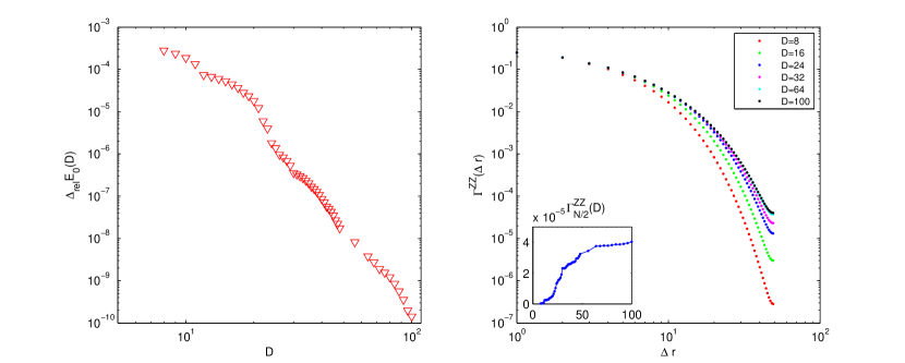
In figure 15 we have plotted the relative energy precision and the correlation functions as functions of $D$. Note that for the ”exact” ground state energy density we have used $E_{0}=-1.401484039$ which is the value obtained by an extrapolation of our own finite $D$ results to infinite $D$. We have done this since the ground state energy that we obtain for $D=100$ is smaller than any other value we have found in the literature, and in particular smaller than the one used as the ”exact” ground state energy in Ref. Pippan et al. (2010).

The correlation functions plotted in figure 15 show non-trivial behaviour around $\Delta r\approx N/2$ where they clearly deviate from exponential decay. The half-chain correlator plotted in the inset seems to converge as a function of $D$ but we do not have compelling evidence for that.

V Conclusions

We have demonstrated the performance of a gradient based algorithm for the simulation of TI spin chains with PBC both for critical and non-critical systems. For critical systems where the correlation length is of the order of the system size, the overall scaling of the computational cost is $O(mnD^{3})+O(n^{2}D^{3})$ and we have given an analysis of the parameter space $\{m,n\}$ with a prescription of how to obtain a quasi-optimal pair $\{m_{opt},n_{opt}\}$. In the special case of a critical system that is simulated by MPS with comparatively small $D$, such that $\tilde{\xi}_{D}\ll N$ holds for the induced correlation length, the overall scaling is given by $O(mD^{3})+O(nD^{3})$. For non-critical systems with a correlation length that is much smaller than the system size, increasing $D$ barely affects the parameters $m$ and $n$ and we can write for the overall scaling $O(D^{3})$. In the last two cases the cost is one factor $N$ less than the one of the algorithm presented in Ref. Pippan et al. (2010). However, for critical systems in the large-$D$ regime, the cost of Ref. Pippan et al. (2010) is improved merely by a factor $N/n$ due to the appearence of $n^{2}$ in the scaling of our algorithm. The precision of our numerical results is comparable with or even better than that of previous algorithms with the same bond dimension. With a TI MPS approximation of the ground state at hand it is possible to develop efficient MPS algorithms for the computation of excitations in TI systems.

VI Acknowledgements

We thank V. Murg, E. Rico and L. Tagliacozzo for valuable discussions. This work was supported by the FWF doctoral program Complex Quantum Systems (W1210) the FWF SFB project FoQuS, the ERC grant QUERG, and the ARC grants FF0668731 and DP0878830.

References

- White (1992) S. R. White, Phys. Rev. Lett. 69, 2863 (1992)
- Rommer and Östlund (1997) S. Rommer and S. Östlund, Phys. Rev. B 55, 2164 (1997)
- Vidal (2004) G. Vidal, Phys. Rev. Lett. 93, 040502 (2004)
- Verstraete et al. (2004) F. Verstraete, D. Porras, and J. I. Cirac, Phys. Rev. Lett. 93, 227205 (2004)
- Verstraete et al. (2008) F. Verstraete, V. Murg, and J. I. Cirac, Advances in Physics 57, 143 (2008)
- Sandvik and Vidal (2007) A. W. Sandvik and G. Vidal, Phys. Rev. Lett. 99, 220602 (2007)
- Pippan et al. (2010) P. Pippan, S. R. White, and H. G. Evertz, Phys. Rev. B 81, 081103(R) (2010)
- Cardy (1996) J. Cardy, Scaling and renormalization in statistical physics (Cambridge University Press, 1996)
- Nishino and Okunishi (1995) T. Nishino and K. Okunishi, Journal of the Physical Society of Japan 64, 4084 (1995)
- Hieida et al. (1997) Y. Hieida, K. Okunishi, and Y. Akutsu, Physics Letters A 233, 464 (1997), ISSN 0375-9601
- Okunishi et al. (1999) K. Okunishi, Y. Hieida, and Y. Akutsu, Phys. Rev. E 59, R6227 (1999)
- Ueda et al. (2006) K. Ueda, T. Nishino, K. Okunishi, Y. Hieida, R. Derian, and A. Gendiar, Journal of the Physical Society of Japan 75, 014003 (2006)
- Vidal (2007) G. Vidal, Phys. Rev. Lett. 98, 070201 (2007)
- McCulloch (2008) I. P. McCulloch (2008), eprint arXiv:0804.2509v1
- Orús and Vidal (2008) R. Orús and G. Vidal, Phys. Rev. B 78, 155117 (2008)
- Pirvu et al. (2010) B. Pirvu, V. Murg, J. I. Cirac, and F. Verstraete, New J. Phys. 12, 025012 (2010)
- Nishino et al. (1996) T. Nishino, K. Okunishi, and M. Kikuchi, Physics Letters A 213, 69 (1996), ISSN 0375-9601
- Andersson et al. (1999) M. Andersson, M. Boman, and S. Östlund, Phys. Rev. B 59, 10493 (1999)
- Tagliacozzo et al. (2008) L. Tagliacozzo, T. R. de Oliveira, S. Iblisdir, and J. I. Latorre, Phys. Rev. B 78, 024410 (2008)
- Pollmann et al. (2009) F. Pollmann, S. Mukerjee, A. M. Turner, and J. E. Moore, Phys. Rev. Lett. 102, 255701 (2009)
- Pirvu et al. (2010) B. Pirvu et al., in preparation (2010)
- Press et al. (2007) W. H. Press, S. A. Teukolsky, W. T. Vetterling, and B. P. Flannery, Numerical Recipes: The Art of Scientific Computing (Cambridge University Press, 2007)
- Lieb et al. (1961) E. Lieb, T. Schultz, and D. Mattis, Annals of Physics 16, 407 (1961)
- White and Huse (1993) S. R. White and D. A. Huse, Phys. Rev. B 48, 3844 (1993)