Optimizing Pulsar Timing Arrays to Maximize Gravitational Wave Single Source Detection: a First Cut

Abstract

Pulsar Timing Arrays (PTAs) use high accuracy timing of a collection of low timing noise pulsars to search for gravitational waves in the microhertz to nanohertz frequency band. The sensitivity of such a PTA depends on (a) the direction of the gravitational wave source, (b) the timing accuracy of the pulsars in the array and (c) how the available observing time is allocated among those pulsars. Here, we present a simple way to calculate the sensitivity of the PTA as a function of direction of a single GW source, based only on the location and root-mean-square residual of the pulsars in the array. We use this calculation to suggest future strategies for the current North American Nanohertz Observatory for Gravitational Waves (NANOGrav) PTA in its goal of detecting single GW sources. We also investigate the affects of an additional pulsar on the array sensitivity, with the goal of suggesting where PTA pulsar searches might be best directed. We demonstrate that, in the case of single GW sources, if we are interested in maximizing the volume of space to which PTAs are sensitive, there exists a slight advantage to finding a new pulsar near where the array is already most sensitive. Further, the study suggests that more observing time should be dedicated to the already low noise pulsars in order to have the greatest positive effect on the PTA sensitivity. We have made a web-based sensitivity mapping tool available at http://gwastro.psu.edu/ptasm.

1 Introduction

Pulsar Timing Arrays (PTAs) (Foster & Backer, 1990) are a practical means of observing gravitational waves (GWs) associated with supermassive ($>10^{8}M_{\odot}$) black holes, or more generally GWs in the nanohertz to microhertz regime arising from any source (Jaffe & Backer, 2003; Jenet et al., 2006a; Sesana & Vecchio, 2010a; Olmez, Mandic, & Siemens, 2010). A PTA is a collection of low timing noise pulsars timed to high accuracy. In such a timing array, GWs may signal their presence through correlated disturbances in measured pulse arrival times. Over the last decade, assessments of expected GW source strengths have remained steady (Sesana & Vecchio, 2010a) while the number of pulsars that can be timed to high precision has increased, and instrumentation, observing technique, and timing precision of known pulsars have all improved (Hobbs et al., 2010). Detection of GWs via pulsar timing is now within striking distance. Properly made strategic choices for observing and/or improving the timing precision of current array pulsars, and searching for new pulsars, can hasten the arrival of the day when the first detection is made and the field of GW astronomy is properly inaugurated.

Strategic optimization depends upon your strategy. Do you want to detect single sources, or a stochastic background? Do you want to maximize the number of sources detected, or maximize the signal-to-noise ratio (SNR) of the sources that you do detect? Here we investigate the sensitivity of a PTA to a single source of GWs and investigate optimization strategies that maximize the number of sources detected. We describe the results of a preliminary investigation into strategies for deploying limited observing time among current array pulsars, and for searching for new pulsars to augment the current array. Our results apply to the search for single sources of GWs(Finn & Lommen, 2010; Yardley et al., 2010), not to stochastic background searches (Jenet et al., 2006b; Anholm et al., 2008; van Haasteren et al., 2009).

After an introduction of the PTA single-source sensitivity calculation and NANOGrav characteristics in §2, we discuss in §3 the consequences of adding pulsars to the array. Further, discussed in §4, is the preliminary study of pulsar timing allocation time. Finally, in §5, we discuss the implications that rise from this study and suggest future research.

2 Calculating PTA Sensitivity

Anticipated GW sources in the nHz-$\mu$Hz band include nearby supermassive black hole binary and triplet systems (Jaffe & Backer, 2003; Sesana & Vecchio, 2010a; Amaro-Seoane et al., 2010). More speculative sources include a primordial stochastic background and bursts from cosmic string cusps and kinks (Damour & Vilenkin, 2001, 2005; Siemens et al., 2006; Siemens, Mandic, & Creighton, 2007; Olmez, Mandic, & Siemens, 2010). All these sources are expected to be isotropically distributed on the sky. Correspondingly we choose to estimate the sensitivity of PTAs as the spatial volume within which a fiducial source would give an SNR greater than a fixed threshold. Such a measure can be made independent of the threshold (but not the fiducial source) by referring the calculated volume to a reference volume calculated for a reference array. In this way we define the relative overall sensitivity $\nu_{overall}$ of a PTA as:

$$\nu_{overall}=\frac{\sum_{i=1}^{n}d(\hat{k}_{i})^{3}}{\sum_{i=1}^{n}d(\hat{k}_{i})_{R}^{3}},$$ (1)

where $d$ is the distance out to which the PTA is sensitive to a source propagating in direction $\hat{k}_{i}$ relative to the reference PTA denoted with a subscript $R$. The limit $n$ is the number of directions along which sensitivity is being measured and can be chosen by the user according to the desired resolution of the resulting sensitivity map. In the maps we constructed in this paper we used HEALPix to construct pixels representing equal surface area, and $n=3072$.

The distance to a fiducial GW source in a fixed direction is inversely proportional to its amplitude SNR $\rho$ as observed in a PTA. Correspondingly, we may use the amplitude SNR of a fiducial source (assuming we have measured the optimal SNR) as a surrogate for the distance of the source

$$d(\hat{k},\rho)=d(\hat{k},\rho_{0})\frac{\rho_{0}}{\rho},$$ (2)

where $d(\hat{k},\rho)$ is the distance to the source when its anticipated SNR is $\rho$, its propagation direction is $\hat{k}$, and $\rho_{0}$ is the amplitude SNR of the fiducial source at distance $d(\hat{k},\rho_{0})$.

Timing noise for typical PTA pulsars is typically white on timescales less than 5–10 years and red on longer timescales (Jenet et al., 2006a; Hobbs, Lyne, & Kramer, 2006). The white contribution to the timing noise is characterized by its root mean square (RMS) residual $\sigma_{j}$. For our approximate analysis here we ignore the red timing noise contribution and assume, for each PTA pulsar, white timing noise characterized by $\sigma_{j}$ for pulsar $j$, and that a single $\sigma_{j}$ characterizes the entire observation.

With this timing noise approximation the contribution from pulsar $j$ to the PTA power SNR in direction $\hat{k}$ is

$$\rho^{2}_{j}(\hat{k},t) =\frac{\tau^{2}_{GW}(\hat{k},t)_{j}}{\sigma_{j}^{2}},$$ (3)

where $\tau_{GW}(\hat{k},t)_{j}$ is the anticipated GW contribution to the residuals in pulsar $j$ from a GW source propagating in direction $\hat{k}$ at time $t$. The anticipated power SNR $\rho^{2}$ of the whole array to sources propagating in direction $\hat{k}$ is the sum over the pulsars

$$\rho^{2}(\hat{k},t) =\Sigma_{j=1}^{n_{p}}\frac{\tau^{2}_{GW}(\hat{k},t)_{j}}{\sigma_{j}^{2}},$$ (4)

where $n_{p}$ is the number of pulsars. Armed with this equation, we set off to find $\tau_{GW}(\hat{k},t)_{j}$.

The timing residuals $\tau_{GW}$ associated with TT-gauge GW metric perturbation $h_{+}\mathbf{e}_{+}+h_{\times}\mathbf{e}_{\times}$ may be written as

$$\tau_{GW}(\hat{k},t)_{j} =F^{+}(\hat{k},\hat{n}_{j})g_{+}(t,L_{j},\hat{k}\cdot\hat{n}_{j})+F^{\times}(\hat{k},\hat{n}_{j})g_{\times}(t,L_{j},\hat{k}\cdot\hat{n}_{j}),$$ (5)

where $\hat{n}_{j}$ is a unit vector pointing to pulsar $j$, $L_{j}$ is the distance to that pulsar, and $\hat{k}$ is the direction of propagation of the GW. $F^{+/\times}$ are given by

$$F^{+}(\hat{k},\hat{n}_{j}) =-\frac{1}{2}\hat{n}_{j}^{T}\mathbf{e}^{+}(\hat{k})\hat{n}_{j},$$ (6)

$$F^{\times}(\hat{k},\hat{n}_{j}) =-\frac{1}{2}\hat{n}_{j}^{T}\mathbf{e}^{\times}(\hat{k})\hat{n}_{j},$$ (7)

where $\hat{n}^{T}$ denotes the transpose of $\hat{n}$, and $\mathbf{e}^{(+)}$ and $\mathbf{e}^{(\times)}$ are the two independent gravitational wave polarization basis tensors,

$$e_{(+)}^{lm}e^{(+)}_{lm}=e_{(\times)}^{lm}e^{(\times)}_{lm}=2$$ (8)

$$e_{(+)}^{lm}\hat{k}_{m}=e_{(\times)}^{lm}\hat{k}_{m}=e_{(+)}^{lm}e^{(\times)}_{lm}=0.$$ (9)

Functions $g_{+}$ and $g_{\times}$ are integrals of $h_{+}$ and $h_{\times}$ as follows (Finn & Lommen, 2010):

$$g_{(+/\times)}(t,L_{j},\hat{k}_{j}\cdot\hat{n}^{j})=\int_{0}^{L_{j}}h_{+/\times}\left(t-(1+\hat{k}\cdot\hat{n}_{j})(L_{j}-\lambda)\right)d\lambda.$$ (10)

Note that we are using geometrized units where $c=G=1$. We have essentially broken up $\tau_{GW}(\hat{k})_{j}$ into terms that depend on geometry ($F$’s) and terms that depend on time ($g$’s). Following (Finn & Lommen, 2010) we assume that a function $f$ exists for which

$$df_{+/\times}(u)/du=h_{+/\times}(u).$$ (11)

We can then do the integral as follows:

$$g_{(+/\times)}(t,L_{j},\hat{k}_{j}\cdot\hat{n}^{j})=\frac{f_{+/\times}(t)}{1+\hat{k}\cdot\hat{n}_{j}}-\frac{f_{+/\times}(t-(1+\hat{k}\cdot\hat{n}_{j})L_{j})}{1+\hat{k}\cdot\hat{n}_{j}}.$$ (12)

The first term is the so-called ‘earth term’, and the second the ‘pulsar term’(Jenet et al., 2004). The pulsar term is delayed from the earth term by $(1+\hat{k}\cdot\hat{n}_{j})L_{j}$ which amounts to hundreds to thousands of years in most cases. For the moment, assume that we are dealing with burst sources whose length is shorter than our observation time (years) for which we only observe the earth term, and that we can thereby ignore the pulsar term. Later we will show that the result we derive here holds for continuous sources, when the pulsar term must be included, as well.

$\tau_{GW}(\hat{k},t,t)_{j}$ depends on time, so what we desire is the time averaged SNR, $\overline{\rho^{2}}$, i.e. the time average of equation 4. We square equation 5 and average over time and all possible polarizations $h_{+}$ and $h_{\times}$. The cross-term $F^{+}(\hat{k},\hat{n}_{j})F^{\times}(\hat{k},\hat{n}_{j})$ vanishes when we average over all polarizations. Also by averaging over all polarizations we find $\overline{g_{+}^{2}}=\overline{g_{\times}^{2}}$. Finally, exploiting time translation symmetry we can write

$$\overline{\rho^{2}_{j}} =A^{2}\left(\frac{F^{(+)2}(\hat{k},\hat{n}_{j})+F^{(\times)2}(\hat{k},\hat{n}_{j})}{\sigma_{j}^{2}(1+\hat{k}\cdot\hat{n}_{j})^{2}}\right),$$ (13)

where $A^{2}$ is a constant independent of the pulsar line-of-sight $\hat{n}_{j}$ or the propagation direction of the GWs $\hat{k}$.

Combining equations 2, 4, 6, 7 and 13 we have our principal result

$$\overline{\rho^{2}(\hat{k})} =A^{2}\sum_{j=1}^{n_{p}}\frac{F^{(+)2}(\hat{k},\hat{n}_{j})+F^{(\times)2}(\hat{k},\hat{n}_{j})}{\sigma_{j}^{2}(1+\hat{k}\cdot\hat{n}_{j})^{2}},$$ (14)

$$=\frac{A^{2}}{4}\sum_{j=1}^{n_{p}}\frac{\left(1-(\hat{k}\cdot\hat{n}_{j})^{2}\right)^{2}}{\sigma_{j}^{2}(1+\hat{k}\cdot\hat{n}_{j})^{2}},$$ (15)

$$=A^{\prime 2}\sum_{j=1}^{n_{p}}\left(\frac{1-\hat{k}\cdot\hat{n}_{j}}{\sigma_{j}}\right)^{2}.$$ (16)

The steps between equations 14 and 15 can be done for any $\hat{k}$, but the result in equation 15 can be seen more readily by assuming the GW is traveling in the $\hat{z}$ direction which gives

$$\mathbf{e}^{+}(\hat{k})=\left|\begin{array}[]{ccc}1&0&0\\ 0&-1&0\\ 0&0&0\end{array}\right|,$$

$$\mathbf{e}^{\times}(\hat{k})=\left|\begin{array}[]{ccc}0&1&0\\ 1&0&0\\ 0&0&0\end{array}\right|,$$

and assuming an arbitrary pulsar direction $\hat{n}_{j}=[n_{x},n_{y},n_{z}]$. The numerator in the sum in equation 14 becomes (after some algebra and trigonometry) $(1-n_{z}^{2})^{2}/4$. For an arbitrary GW direction, $\hat{k}$, the numerator generalizes to $(1-(\hat{k}\cdot\hat{n}_{j})^{2})^{2}/4$. In other words, the quantity that matters is the projection of the pulsar direction vector onto the direction of propagation of the GW.

Equation 16 will allow us to compare various PTAs independently of the details of the input source ($g_{+}$ and $g_{\times}$ as shown in equation 5) and then putting this into equation 1:

$$\nu_{overall} =\frac{\Sigma_{i=1}^{n}\overline{\rho^{2}(\hat{k_{i}})}^{3/2}}{\Sigma_{i=1}^{n}\overline{\rho_{R}^{2}(\hat{k_{i}})}^{3/2}},$$ (17)

where $\overline{\rho_{R}^{2}}$ refers to the reference PTA, and, as in equation 1, the $n$ is the resolution of the calculation, i.e. the number of pixels in the map of $\overline{\rho^{2}(\hat{k_{i}})}$. $\nu_{overall}$ is what we are calling the ‘volume sensitivity’ and represents the ratio of the volumes to which two different PTAs are sensitive.

A related quantity which we will utilize later, ${\nu}(\hat{k})$, represents the comparison of the sensitivity of two arrays as a function of the GW propagation direction $\hat{k}$,

$$\nu(\hat{k}) =\frac{\overline{\rho^{2}(\hat{k})}^{3/2}}{\overline{\rho_{R}^{2}(\hat{k})}^{3/2}}.$$ (18)

Note that rather than plotting $\nu(\hat{k})$ as a function of GW propagation direction $\hat{k}$ we will plot $\tilde{\nu}(\hat{s})$ where $\hat{s}$ is the direction of the GW source in the sky, $\hat{s}=-\hat{k}$, and $\tilde{\nu}(\hat{s})=\nu(-\hat{k})$.

The quantity

$$P^{2}(\hat{k}) =\frac{\overline{\rho^{2}(\hat{k})}}{\max_{\hat{k}}\overline{\rho^{2}(\hat{k})}}$$ (19)

lends itself to interpretation as the PTA antenna pattern: i.e., it is proportional to the signal power absorbed by the detector from a source propagating in the direction $\hat{k}$, measured relative to the source direction for which the greatest power is absorbed. As with $\nu(\hat{k})$, $\tilde{P^{2}}(\hat{s})=P^{2}({-\hat{k}})$. Figure 1 shows “source-averaged” antenna pattern $\tilde{P}^{2}(\hat{s})$ for the NANOGrav PTA, whose member pulsars and their RMS timing residuals at the time of writing are provided in Table 1. We have also made available a web-based tool for computing sensitivity maps for an arbitrary array of pulsars at this URL.

Figure 1: Antenna pattern $\tilde{P}^{2}(\hat{s})$ (defined in the text following equation 19) of the NANOGrav PTA is shown in equatorial coordinates. In other words, this shows the sensitivity of the NANOGrav PTA to single GW sources as a function of location of the source. The diamonds show the location of the pulsars in the array.

As evident from Figure 1 the sensitivity of the NANOGrav PTA is heavily biased to the region between 12 and 24 hours right ascension, yet fairly symmetric about the equatorial plane. Not surprisingly this region represents both the highest concentration of pulsars and also the location of the lowest noise pulsars.

Rather than average over all possible GWs propagating in direction $\hat{k}$ we can restrict attention to any particularly interesting class of sources. Consider, for example, the radiation from a circular binary consisting of two supermassive black holes. For systems like these the radiation is approximately periodic over any reasonable observational timescale (Jenet et al., 2006b; Sesana & Vecchio, 2010b) and

$$\tau_{GW}(\hat{k})_{j}\propto\cos\omega t-\cos\omega\left[t-(1-\hat{k}\cdot\hat{n}_{j})L_{j}\right],$$ (20)

where $\omega$ is the GW angular frequency. Even in the best of circumstances pulsar distances are known to no better than 10% (Cordes & Lazio, 2002), in which case the phase $\omega L_{j}$ is uncertain by many times $2\pi$ for $\omega$ of interest. If we average $\tau_{GW}(\hat{k})_{j}$ over the typical uncertainty in distance we find the contribution owing to the term involving $L_{j}$, the pulsar term, vanishes and we are left with $\cos^{2}\omega t$ which, averaged over time, tends to 0.5, a constant. As long as the uncertainty in pulsar distance is greater than the light travel time over the duration of the observation these same considerations will hold for any source that a PTA can detect: i.e., averaged over the uncertainty in pulsar distances the pulsar term contribution to $\tau^{2}$ will vanish and we can again ignore the second term on the right-hand side of equation 12 as we did to obtain the result shown in equations 16. Note that in the case of $\hat{k}\cdot\hat{n}=1$ the earth and the pulsar terms exactly cancel and the sensitivity $\overline{\rho^{2}(\hat{k})}=0$ as is shown in equation 14.

3 Addition of Pulsars

Adding a new pulsar to an existing array increases the array’s overall sensitivity. Equation 17 shows how the array’s sensitivity increases as a function of a new pulsar’s sky location and timing residual noise RMS. While we do not have the freedom to choose where we will find the next good millisecond pulsar, we do have the freedom to choose where we will look. With this in mind we consider how the sensitivity of the NANOGrav PTA would be increased by the addition of a single pulsar whose timing residual noise of 200 ns RMS is equal to the current array’s median.

Figure  2 shows the sensitivity $\nu_{overall}$ as calculated using equation 17 as a function of the location of an addition to the NANOGrav PTA of a single pulsar with 200 ns timing noise RMS. As is confirmed by the figure, an additional pulsar will improve the PTA sensitivity regardless of its location on the sky, but the improvement represents less than a 6% increase in sensitivity volume (the volume of space from which we can detect sources) in all cases. However, some pulsar locations will improve it more than others. An additional pulsar in the region in which the PTA is already most sensitive improves the sensitivity volume the greatest. This seems appropriate considering that the volume of sensitivity goes as $d^{3}$. So, if a distance that is already large is doubled, the volume increase will be a larger factor than if a small distance were doubled. However, the volume sensitivity varied by only 6% as we moved the additional pulsar all over the sky, so it may be wisest to search where one is most likely to find pulsars, such as in the galactic plane. One aspect which has not been addressed in this manuscript is the coherence of the GW signal between pulsars, i.e. the fact that pulsars in similar directions in the sky will show higher correlation between their GW signals than those in different parts of the sky (see eq. 12). In addition, in order to confirm that the detected signal is a GW and not, for example, an error in earth’s ephemerides, or a terrestrial clock, we will need pulsars in different parts of the sky to confirm that the spatial signature of the detected signal is quadrupolar in nature and not dipolar (ephemerides error) or monopolar (clock error). Further study which includes these considerations is necessary to determine the optimum strategy.

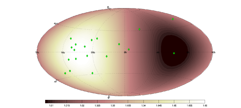
Figure 2: Shown, the relative sensitivity improvement $\nu_{overall}$ (equation 17) of the NANOGrav PTA caused by the addition of a pulsar, as a function of the location of that added pulsar, in equatorial coordinates. Every pixel represents the relative sensitivity improvement caused by an additional pulsar at that location in the sky.

4 Optimization With Time Constraints

The NANOGrav PTA at the time of writing involves 19 pulsars whose timing residuals range from 54 ns to 2.2 $\mu$s. Monitoring each pulsar requires some fraction of the available observing time, which is a valuable resource. How should the available observing time be distributed among the different pulsars to optimize the NANOGrav PTA’s sensitivity? To explore this question we divide the NANOGrav PTA pulsars into “low-noise” (timing residual noise less than 200 ns) and“high-noise” (timing residual noise greater than 200 ns) groups, and evaluate the array sensitivity when we increase the fraction of observing time spent on low-noise pulsars at the expense of high-noise pulsars, and vice versa.

For a typical timing array pulsar the RMS timing residual noise, $\sigma$, is inversely proportional to the square-root of the time spent observing the pulsar, i.e., $\sigma\propto t^{-1/2}$ (Verbiest, 2009). The current NANOGrav timing program spends an approximately equal amount of time on each pulsar in the array. We consider two alternatives: spending twice as much observing time on pulsars in the high-noise group as on pulsars in the low-noise group, and the opposite case of twice as much observing time on pulsars in the low-noise group as on pulsars in the high-noise group. This translates to the observing time of one group being multiplied by $\frac{4}{3}$ while the observing time of the other group is multiplied by $\frac{2}{3}$. This, as RMS and $t$ are related above, results in an decrease in RMS of the first group by $\sqrt{3/4}$ and an increase in RMS of the second group by $\sqrt{3/2}$. (In both cases the time spent observing the single pulsar with timing residual noise of exactly 200 ns is left fixed.) Figure  3 shows the change in volume sensitivity enacted by these adjustments as a function of GW propagation direction, $\hat{s}$. What we plot is $\tilde{\nu}(\hat{s})$ where the reference array in the denominator (see equation 18) consists of the NANOGrav pulsars shown in Table 1. The array used in the numerator is one in which the adjustments described above have been assumed.

NANOGrav Pulsars
	Pulsar	RMS($\mu$s)
1	J0030+0451	0.300
2	J0218+4232	0.830
3	J0613-0200	0.110
4	J1012+5307	0.540
5	J1455-3330	0.960
6	J1600-3053	0.190
7	J1640+2224	0.110
8	J1643-1224	1.100
9	J1713+0747	0.055
10	J1738+0333	0.200
11	J1741+1300	0.140
12	J1744-1134	0.130
13	J1857+0943	0.066
14	J1909-3744	0.054
15	J1918-0642	0.960
16	J1939+2134	0.080
17	J2019+2425	0.910
18	J2145-0750	0.750
19	J2317+1439	0.369
PPTA Pulsars not part of NANOGrav
20	J0437-4715	0.10
21	J0711-6830	1.00
22	J1022+1001	0.50
23	J1024-0719	1.00
24	J1045-4509	1.00
25	J1603-7202	0.50
26	J1730-2304	1.00
27	J1732-5049	1.00
28	J1824-2452	1.00
29	J2124-3358	1.00
30	J2129-5721	1.00
31	J2145-0750	0.30

Table 1: The NANOGrav pulsars with the current RMS timing values at the time of writing. ⁵This is a particular characterization of these NANOGrav pulsars based on communications at the time of this writing with the North American Nanohertz Observatory for Gravitational Waves. It is not a definitive characterization. We are not presenting the data associated with these pulsars but rather using them as an example of a realistic PTA. ⁶RMS values for EPTA pulsars from Hobbs et al. (2009).

As is noticeable from Figure  3 (with two scales required for plot structure), bettering the already good pulsars improves the overall array sensitivity volume by a factor of 1.5 ($\nu_{overall}=1.5$, see equation 17 for definition of $\nu_{overall}$), while bettering the bad pulsars has quite the opposite effect actually worsening the current sensitivity volume ($\nu_{overall}=0.6$). The key to understanding this result is in noting that SNR $\rho$, residual response $\tau$ and RMS $\sigma$ are related to each other approximately as follows

$$\rho\propto\frac{\tau}{\sigma},$$ (21)

and $\tau=\tau_{0}(d_{0}/d)$ where $\tau_{0}$ is the amplitude of the residual at earth when the source is at distance $d_{0}$. Therefore

$$\rho\propto\frac{\tau_{0}}{\sigma d},$$ (22)

or for a fixed SNR $\rho$ required for detection, the distance out to which we could detect a source, $d$, is inversely proportional to the RMS $\sigma$

$$d\propto 1/\sigma.$$ (23)

The argument then is similar to that which we made in §3, that volume sensitivity goes as $d^{3}$ so halving an already small RMS $\sigma$ increases the volume sensitivity by a much larger factor than halving a larger RMS $\sigma$.

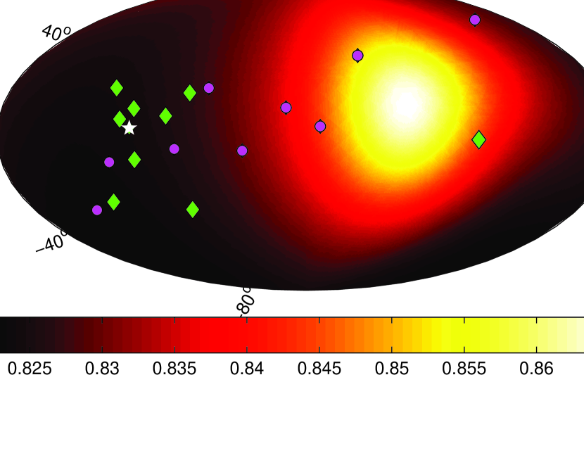
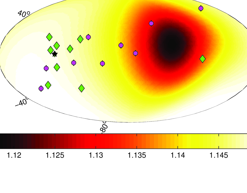
Figure 3: Sensitivity improvement compared to the current NANOGrav pulsars and current NANOGrav pulsar RMS timing values as a function of GW propagation direction $\hat{s}$. In both panels we plot $\tilde{\nu}(\hat{s})$ as defined by equation 18 and the text immediately thereafter. On the left we improve the RMS of the high-noise pulsars and obtain a volume sensitivity, $\nu_{overall}=0.6$. On the right we improve the RMS of the low-noise pulsars and obtain a volume sensitivity, $\nu_{overall}=1.5$. Diamonds are the low-noise pulsars, circles are the high-noise pulsars. The median pulsar whose RMS we did not alter is a pentagram. All coordinates are equatorial. Please note the scales of the two diagrams are different to allow the reader to see the structure of the plots.

We can use the same formalism to determine the value of adding more pulsars to the array and can use it to ascertain the value of the International Pulsar Timing Array (IPTA) a collaboration formed of NANOGrav, the PPTA and the the European Pulsar Timing Array (EPTA). In table 1 below the NANOGrav pulsars we have shown the Parkes Pulsar Timing Array pulsars, not including those overlapping with NANOGrav, as published in the status paper by Hobbs et al. (2009). If solely PSR J0437-4715 is added to the NANOGrav array, the volume sensitivity increases by 7%. If all the PPTA pulsars listed are added to the NANOGrav array, the volume sensitivity increases by 10%. If instead we imagine an improved situation in which the PPTA pulsars listed are added with 200ns RMS, with the exception of PSR J0437-4715 which we add at its actual RMS of 100 ns, the volume sensitivity is increased by 35%, ie 35% more volume of space is sampled for the same GW source type. At the time of writing the European Pulsar Timing Array (EPTA) pulsars for which RMSs are available(Ferdman et al., 2010) are already included in this list. Their typical RMSs are slightly higher than the values shown here, but there are several reasons to expect that within a year the EPTA RMSs will be markedly reduced and that the pulsars will contribute significantly to this list. First, the Large European Array of Pulsars (LEAP) project which expects first light in late 2010 will create a “tied-array” mode for the 5 European 100-m class dishes into a single instrument, rivaling the sensitivity of Arecibo, but with larger sky coverage. Furthermore, the data reported on by Ferdman et al. (2010) represent new instrumentation at all 5 telescopes, so one can expect significant improvement with characterization and optimization of those instruments.

5 Discussion and Conclusion

Given the goal to directly detect GWs, the optimization of pulsar timing arrays should be well understood. Figure 2 suggests that for the sake of GW detection we may not need to “fill in” regions of the sky currently devoid of PTA pulsars, but that rather a clustering of good pulsars in one region yields the gratest number of detectable GW sources. The figure shows the sensitivity (volumetric) gain produced by adding a new pulsar to the array as a function of the location of the added pulsar. The current pulsars in the array are clustered around 18h right ascension and 0 declination (as shown by green diamonds on the figure) and in fact the greatest improvement in the volume to which the array is sensitive is produced by adding a new pulsar near that already existing cluster of pulsars, although the range of improvement is modest in all cases (from improving it not at all to improving it by 6%). Here we suggest that if the goal is to maximize the volume of space to which we are sensitive to GW sources the location with highest concentration of pulsars is slightly favored over other locations, but does not make a significant difference. So perhaps efforts to “fill in the gaps” in the spatial arrangements of PTAs are unfounded. However, any new pulsar, regardless of its location, is beneficial to the scientific community. Continuing research is needed on this particular area to optimize pulsar searches for PTA goals.

Our initial findings indicate that the sensitivity to burst and continuous GWs can be significantly improved by observing longer the pulsars for which we already have good timing values. In other words, it is found that the intuitive thing to do, observing longer the pulsars that we do not have good timing values for, significantly decreases our sensitivity to GWs by almost 50% (Figure  3). This suggestion taken to an extreme yields the ridiculous result that it is best to spend all observing time on a signal pulsar. The sensitivity plot in this case would be the familiar beam pattern of a single pulsar, but if somehow GWs could be detected with a single pulsar, spending all our time on this one best pulsar, assuming the RMS reduces as the square-root of observing time, would in fact maximize the volume of space to which we are sensitive. We discussed in §3 that this strategy neglects issues with confirming the detection as distinct from clock, ephemerides, and other errors, so more work must be done to optimize observing strategies, but this work clearly indicates that convention may not be the best means to a discovery. In particular, as the PTA is being optimized, what should the observing strategy be? Is the answer different depending on whether our aim is to detect single sources or a stochastic background. Presented here is a crucial first step toward answering these questions.

References

- Amaro-Seoane et al. (2010) Amaro-Seoane, P., Sesana, A., Hoffman, L., Benacquista, M., Eichhorn, C., Makino, J., & Spurzem, R. 2010, MNRAS, 402, 2308
- Anholm et al. (2008) Anholm, M., Ballmer, S., Creighton, J. D. E., Price, L. R., & Siemens, X. 2008, ArXiv e-prints
- Cordes & Lazio (2002) Cordes, J. M., & Lazio, T. J. 2002, astro-ph/0207156
- Damour & Vilenkin (2001) Damour, T., & Vilenkin, A. 2001, Phys. Rev. D, 64, 064008
- Damour & Vilenkin (2005) Damour, T., & Vilenkin, A. 2005, Phys. Rev. D, 71, 063510
- Ferdman et al. (2010) Ferdman, R. D., van Haasteren, R., Bassa, C. G., Burgay, M., Cognard, I., Corongiu, A., D’Amico, N., Desvignes, G., Hessels, J. W. T., Janssen, G. H., Jessner, A., Jordan, C., Karuppusamy, R., Keane, E. F., Kramer, M., Lazaridis, K., Levin, Y., Lyne, A. G., Pilia, M., Possenti, A., Purver, M., Stappers, B., Sanidas, S., Smits, R., & Theureau, G. 2010, Classical and Quantum Gravity, 27, 084014
- Finn & Lommen (2010) Finn, L. S., & Lommen, A. N. 2010, ApJ, 718, 1400
- Foster & Backer (1990) Foster, R. S., & Backer, D. C. 1990, ApJ, 361, 300–308
- Hobbs, Lyne, & Kramer (2006) Hobbs, G., Lyne, A., & Kramer, M. 2006, Chinese Journal of Astronomy and Astrophysics Supplement, 6, 169
- Hobbs et al. (2010) Hobbs, G., Archibald, A., Arzoumanian, Z., Backer, D., Bailes, M., Bhat, N. D. R., Burgay, M., Burke-Spolaor, S., Champion, D., Cognard, I., Coles, W., Cordes, J., Demorest, P., Desvignes, G., Ferdman, R. D., Finn, L., Freire, P., Gonzalez, M., Hessels, J., Hotan, A., Janssen, G., Jenet, F., Jessner, A., Jordan, C., Kaspi, V., Kramer, M., Kondratiev, V., Lazio, J., Lazaridis, K., Lee, K. J., Levin, Y., Lommen, A., Lorimer, D., Lynch, R., Lyne, A., Manchester, R., McLaughlin, M., Nice, D., Oslowski, S., Pilia, M., Possenti, A., Purver, M., Ransom, S., Reynolds, J., Sanidas, S., Sarkissian, J., Sesana, A., Shannon, R., Siemens, X., Stairs, I., Stappers, B., Stinebring, D., Theureau, G., van Haasteren, R., van Straten, W., Verbiest, J. P. W., Yardley, D. R. B., & You, X. P. 2010, Classical and Quantum Gravity, 27, 084013
- Hobbs et al. (2009) Hobbs, G. B., Bailes, M., Bhat, N. D. R., Burke-Spolaor, S., Champion, D. J., Coles, W., Hotan, A., Jenet, F., Kedziora-Chudczer, L., Khoo, J., Lee, K. J., Lommen, A., Manchester, R. N., Reynolds, J., Sarkissian, J., van Straten, W., To, S., Verbiest, J. P. W., Yardley, D., & You, X. P. 2009, PASA, 26, 103
- Jaffe & Backer (2003) Jaffe, A. H., & Backer, D. C. 2003, ApJ, 583, 616–631
- Jenet et al. (2004) Jenet, F. A., Lommen, A., Larson, S. L., & Wen, L. 2004, ApJ, 606, 799–803
- Jenet et al. (2006a) Jenet, F. A., Hobbs, G. B., van Straten, W., Manchester, R. N., Bailes, M., Verbiest, J. P. W., Edwards, R. T., Hotan, A. W., Sarkissian, J. M., & Ord, S. M. 2006a, ApJ, 653, 1571–1576
- Jenet et al. (2006b) Jenet, F. A., Hobbs, G. B., van Straten, W., Manchester, R. N., Bailes, M., Verbiest, J. P. W., Edwards, R. T., Hotan, A. W., Sarkissian, J. M., & Ord, S. M. 2006b, ApJ, 653, 1571
- Olmez, Mandic, & Siemens (2010) Olmez, S., Mandic, V., & Siemens, X. 2010, ArXiv e-prints
- Sesana & Vecchio (2010a) Sesana, A., & Vecchio, A. 2010a, Classical and Quantum Gravity, 27, 084016
- Sesana & Vecchio (2010b) Sesana, A., & Vecchio, A. 2010b, Phys. Rev. D, 81, 104008
- Siemens et al. (2006) Siemens, X., Creighton, J., Maor, I., Majumder, S. R., Cannon, K., & Read, J. 2006, Phys. Rev. D, 73, 105001
- Siemens, Mandic, & Creighton (2007) Siemens, X., Mandic, V., & Creighton, J. 2007, Physical Review Letters, 98, 111101
- van Haasteren et al. (2009) van Haasteren, R., Levin, Y., McDonald, P., & Lu, T. 2009, MNRAS, 395, 1005
- Verbiest (2009) Verbiest, J. P. W. 2009, ArXiv e-prints
- Yardley et al. (2010) Yardley, D. R. B., Hobbs, G. B., Jenet, F. A., Verbiest, J. P. W., Wen, Z. L., Manchester, R. N., Coles, W. A., van Straten, W., Bailes, M., Bhat, N. D. R., Burke-Spolaor, S., Champion, D. J., Hotan, A. W., & Sarkissian, J. M. 2010, MNRAS, 407, 669