An R-parity conserving radiative neutrino mass model
without right-handed neutrinos

Abstract

The model proposed by A. Zee (1986) and K. S. Babu (1988) is a simple radiative seesaw model, in which tiny neutrino masses are generated at the two-loop level. We investigate a supersymmetric extension of the Zee-Babu model under R-parity conservation. The lightest superpartner particle can then be a dark matter candidate. We find that the neutrino data can be reproduced with satisfying current data from lepton flavour violation even in the scenario where not all the superpartner particles are heavy. Phenomenology at the Large Hadron Collider is also discussed.

Although the standard model (SM) has been successful in describing phenomena below 100 GeV, the Higgs sector has not been confirmed yet. The Higgs boson is expected to be lighter than one TeV from the unitarity argument, so that it can be explored at the CERN Large Hadron Collider (LHC). On the other hand, we require new physics beyond the SM because of several reasons, such as the quadratic divergence problem, the origin of tiny masses of neutrinos, the existence of dark matter (DM), and so on. It is interesting to consider a scenario where these problems are simultaneously solved at the TeV scale, as such a scenario is directly testable at the LHC or future colliders such as the International Linear Collider (ILC) and the Compact Linear Collider (CLIC). In such a case, it is plausible that the Higgs sector is closely related to the detail of physics beyond the SM.

One of the important motivations to consider physics beyond the SM is to explain the origin of tiny neutrino masses. The seesaw mechanism is known to be a simple method of generating neutrino masses at the tree level, in which tiny masses of the (left-handed) neutrinos may be obtained from very heavy right-handed neutrinos (type I)type1 , a heavy triplet Higgs boson (type II)type2 , or a heavy triplet fermion (type III)type3 . However, the mass scale of these fields is much higher than the TeV scale; naively at around $\mathcal{O}(10^{6-15})\;\text{GeV}$, unless the coupling constants between lepton doublets and these new heavy fields are taken to be unnaturally small. Such a high scale is far from experimental reach.

Radiative seesaw models, where neutrino masses are generated at the quantum corrections, are alternative attractive scenarios to generate tiny neutrino masseszee ; zee-2loop ; babu-2loop ; Krauss:2002px ; Ma:2006km ; Aoki:2008av . Masses of new particles in these models can be as low as the TeV scale, so that they are expected to be directly testable at current and future collider experiments. One of the characteristic features of these models is an extended Higgs sector. Another feature is the Majorana nature, either introducing lepton number violating couplings or introducing right-handed neutrinos.

The original model for radiative neutrino mass generation was first proposed by A. Zeezee , where neutrino masses are generated at the one-loop level by adding an extra $\text{SU}(2)_{\text{L}}$ doublet scalar field and a charged singlet scalar field with lepton number violating couplings to the SM particle entries. Phenomenology of this model has been studied in Ref. zee-ph1 . However, it turned out that it was difficult to reproduce the current data for neutrino oscillation in this original modelzee-nu . Some extensions have been discussed in Ref. zee-variation .

The simplest successful model today may be the one proposed by A. Zeezee-2loop and K. S. Babubabu-2loop , in which two kinds of $\text{SU}(2)_{\text{L}}$ singlet scalar fields are introduced; i.e., a singly charged scalar boson and a doubly charged one. These fields carry lepton number of two unit. In this model, which we refer to as the Zee-Babu model, the neutrino masses are generated at the two-loop level. Phenomenology of this model has been discussed in Refs. macesanu ; aristizabal ; nebot ; ohlsson ; ak-letter . Apart from the Zee-Babu model, there is also another type of radiative seesaw modelsKrauss:2002px ; Ma:2006km ; Aoki:2008av , where TeV-scale right-handed neutrinos are introduced with the odd charge under the discrete $Z_{2}$ symmetry. In these models, the $Z_{2}$ symmetry protects the decay of the lightest $Z_{2}$ odd particle, which can be a candidate of DM. This is an advantage of this class of modelsknt_dm ; ma_dm ; aks_dm . On the other hand, in the Zee-Babu model there is no such a discrete symmetry and no neutral new particle, so that there is no DM candidate.

In this Letter, we investigate a supersymmetric extension of the Zee-Babu model. By introducing supersymmetry (SUSY), the quadratic divergence in the one-loop correction to the mass of the Higgs boson can be eliminated automatically. In addition, a discrete symmetry, which is so called the R-parity, is imposed in our model to forbid the term which causes the dangerous proton decay. The R-parity also guarantees the stability of the lightest super partner particle (LSP) such as the neutralino, which may be identified as a candidate of DM. We find that there are allowed parameter regions in which the current neutrino oscillation data can be reproduced under the constraint from the lepton flavour violation (LFV) data. In addition, this model provides quite interesting phenomenological signals in the collider physics; i.e., the existence of singly as well as doubly charged singlet scalar bosons and their SUSY partner fermions. Such an allowed parameter region also appears even when new particles and their partners are as light as the electroweak scale. We also discuss the outline of phenomenology for these particles at the LHC.

In the original (non-SUSY) Zee-Babu modelzee-2loop ; babu-2loop , two kinds of $\text{SU}(2)_{\text{L}}$ singlet fields $\omega^{-}$ ($Y=-1$) and $\kappa^{--}$ ($Y=-2$) are introduced. The Yukawa interaction and the scalar potential are given by

$$\mathcal{L}=-\sum_{i,j=1}^{3}f_{ij}\bar{\ell}_{Li}^{c}\cdot\ell_{Lj}\omega^{+}-\sum_{i,j=1}^{3}g_{ij}\bar{e}_{Ri}e_{Rj}^{c}\kappa^{--}-\mu_{B}\omega^{-}\omega^{-}\kappa^{++}+\text{h.c.}-V^{\prime}-V_{\text{SM}}\;,$$ (1)

where $V_{\text{SM}}$ is the Higgs potential of the SM, $\ell_{Li}$ are lepton doublets, $e_{Ri}$ are right-handed charged leptons, the indices $i$, $j$ are the flavour indices, the dot product of the fields denotes the antisymmetric contract of the $\text{SU}(2)_{\text{L}}$ indices i.e. $\bar{\ell}_{Li}^{c}\cdot\ell_{Lj}\equiv\sum_{\alpha,\beta=1}^{2}\epsilon_{\alpha\beta}\bar{\ell}_{Li}^{\alpha c}\ell_{Lj}^{\beta}$, and all the scalar couplings with respect to $\omega^{-}$ and $\kappa^{--}$ other than $\omega^{-}\omega^{-}\kappa^{++}$ are in $V^{\prime}$. Notice that lepton number conservation is broken only by the term of $\mu_{B}$. The neutrino mass matrix is generated via two-loop diagrams as shown in Fig. 1. The induced neutrino mass matrix is computed as

$$(m_{\nu})_{ij}=\left(\frac{1}{16\pi^{2}}\right)^{2}\sum_{k,l=1}^{3}\frac{16\mu_{B}f_{ik}(m_{e})_{k}g_{kl}(m_{e})_{l}f_{jl}}{m_{\kappa}^{2}}I(m_{\omega},(m_{e})_{k}|m_{\omega},(m_{e})_{l}|m_{\kappa})\;,$$ (2)

where $(m_{e})_{i}$ are charged lepton masses, and the induced mass matrix $(m_{\nu})_{ij}$ is defined in the effective Lagrangian as

$$\mathcal{L}_{\nu}=-\sum_{i,j=1}^{3}\frac{1}{2}(\overline{\nu}^{c}_{L})_{i}(m_{\nu})_{ij}(\nu_{L})_{j}+{\rm h.c.},$$ (3)

and $I(m_{11},m_{12}|m_{21},m_{22}|M)$ is the two-loop integral function defined as

$$I(m_{11},m_{12}|m_{21},m_{22}|M)$$

$$=\frac{1}{\pi^{4}}\int d^{4}p\int d^{4}q\frac{1}{(p^{2}+m_{11}^{2})}\frac{1}{(p^{2}+m_{12}^{2})}\frac{1}{(q^{2}+m_{21}^{2})}\frac{1}{(q^{2}+m_{22}^{2})}\frac{M^{2}}{((p+q)^{2}+M^{2})}\;.$$ (4)

Following Refs. vanderBij:1983bw , one can evaluate the function $I(m_{11},m_{12}|m_{21},m_{22}|M)$ as

$$I(m_{11},m_{12}|m_{21},m_{22}|M)$$

$$=\frac{M^{4}\left\{I(m_{12}|m_{22}|M)-I(m_{11}|m_{22}|M)-I(m_{12}|m_{21}|M)+I(m_{11}|m_{21}|M)\right\}}{(m_{11}^{2}-m_{12}^{2})(m_{21}^{2}-m_{22}^{2})}\;,$$ (5)

where

$$I(m_{1}|m_{2}|M)=-\left\{\frac{m_{1}^{2}}{M^{2}}f\left(\frac{m_{2}^{2}}{m_{1}^{2}},\frac{M^{2}}{m_{1}^{2}}\right)+\frac{m_{2}^{2}}{M^{2}}f\left(\frac{m_{1}^{2}}{m_{2}^{2}},\frac{M^{2}}{m_{2}^{2}}\right)+f\left(\frac{m_{1}^{2}}{M^{2}},\frac{m_{2}^{2}}{M^{2}}\right)\right\}\;.$$ (6)

The function $f(x,y)$ is give by

$$f(x,y)= -\frac{1}{2}\ln x\ln y-\frac{1}{2}\left(\frac{x+y-1}{D}\right)$$

$$\times\left\{\mathrm{Li}_{2}\left(\frac{-\sigma_{-}}{\tau_{+}}\right)+\mathrm{Li}_{2}\left(\frac{-\tau_{-}}{\sigma_{+}}\right)-\mathrm{Li}_{2}\left(\frac{-\sigma_{+}}{\tau_{-}}\right)-\mathrm{Li}_{2}\left(\frac{-\tau_{+}}{\sigma_{-}}\right)\right.$$

$$\phantom{Space}\left.+\mathrm{Li}_{2}\left(\frac{y-x}{\sigma_{-}}\right)+\mathrm{Li}_{2}\left(\frac{x-y}{\tau_{-}}\right)-\mathrm{Li}_{2}\left(\frac{y-x}{\sigma_{+}}\right)-\mathrm{Li}_{2}\left(\frac{x-y}{\tau_{+}}\right)\right\}\;,$$ (7)

where $D$, $\sigma_{\pm}$ and $\tau_{\pm}$ are

$$D= \sqrt{1-2(x+y)+(x-y)^{2}}\;,$$

$$\sigma_{+}= \frac{1}{2}(1-x+y+D)\;,\quad\tau_{+}=\frac{1}{2}(1+x-y+D)\;,\quad$$ (8)

$$\sigma_{-}= \frac{1}{2}(1-x+y-D)\;,\quad\tau_{-}=\frac{1}{2}(1+x-y-D)\;,\quad$$

and $\text{Li}_{2}(x)$ is the dilogarithm function defined as

$$\text{Li}_{2}(x)=-\int_{0}^{x}\frac{\ln(1-t)}{t}dt\;.$$ (9)

We note that in the limit of $m_{12}=m_{22}=0$ and $m_{11}=m_{21}=m_{\omega}$ the above function $I(m_{11},m_{12}|m_{21},m_{22}|M)$ has the same form as the function given in Refs. macesanu ; aristizabal ,

$$I(m_{\omega},0|m_{\omega},0|m_{\kappa})=-\int_{0}^{1}dx\int_{0}^{1-x}dy\frac{r}{x+(r-1)y+y^{2}}\ln\frac{y(1-y)}{x+ry}\;,$$ (10)

where $r=m_{\kappa}^{2}/m_{\omega}^{2}$. One can approximately estimate the above function as

$$I(m_{\omega},0|m_{\omega},0|m_{\kappa})\sim\begin{cases}2.8r\left(r+0.31\right)^{-1.5}\;,&(r\gtrsim 1)\\ 1.98r\left(r+0.12\right)^{-0.23}\;,&(r<1)\\ \end{cases}\;.$$ (11)

Details of the Zee-Babu model have been studied in the literaturemacesanu ; aristizabal ; nebot ; ohlsson . It is known that the model can reproduce the present neutrino data with satisfying constraints from the LFV.

Figure 1: The two-loop diagram relevant to the neutrino mass matrix.

We turn to the SUSY extension of the Zee-Babu model. The $\text{SU}(2)_{\text{L}}$ singlet chiral superfields $\Omega_{R}^{c}$, $\Omega_{L}$, $K_{L}$, and $K_{R}^{c}$ are added to the superfields in the minimal supersymmetric standard model (MSSM), whose details are shown in Table. 1. Notice that although the non-SUSY Zee-Babu model includes only two $\text{SU}(2)_{\text{L}}$ singlet scalars these four chiral fields are required in the SUSY model. If only $\Omega_{R}^{c}$ and $K_{L}$ are introduced in the model, their fermion components are massless and the model is ruled out. By introducing additional fields $\Omega_{L}$ and $K_{R}^{c}$ such massless fermions can be massive, and furthermore the model becomes anomaly free.

Table 1: Particle properties of relevant chiral superfields.

	Spin 0	Spin 1/2	$\text{SU(3)}_{\text{C}}$	$\text{SU(2)}_{\text{L}}$	$\text{U(1)}_{\text{Y}}$	Electric charge	Lepton number
$L_{i}$	$\tilde{\ell}_{Li}=\begin{pmatrix}\tilde{\nu}_{Li}\\ \tilde{e}_{Li}\end{pmatrix}$	$\ell_{Li}=\begin{pmatrix}\nu_{Li}\\ e_{Li}\end{pmatrix}$	1	2	$-\frac{1}{2}$	$\begin{pmatrix}0\\ -1\end{pmatrix}$	1
$E_{i}^{c}$	$\tilde{e}_{Ri}^{*}$	$(e_{R})^{c}$	1	1	1	1	$-1$
$\Phi_{d}$	$\phi_{d}=\begin{pmatrix}\phi_{d}^{0}\\ \phi_{d}^{-}\end{pmatrix}$	$\tilde{h}_{d}=\begin{pmatrix}\tilde{h}_{d}^{0}\\ \tilde{h}_{d}^{-}\end{pmatrix}$	1	2	$-\frac{1}{2}$	$\begin{pmatrix}0\\ -1\end{pmatrix}$	0
$\Phi_{u}$	$\phi_{u}=\begin{pmatrix}\phi_{u}^{+}\\ \phi_{u}^{0}\end{pmatrix}$	$\tilde{h}_{u}=\begin{pmatrix}\tilde{h}_{u}^{+}\\ \tilde{h}_{u}^{0}\end{pmatrix}$	1	2	$\frac{1}{2}$	$\begin{pmatrix}1\\ 0\end{pmatrix}$	0
$\Omega_{R}^{c}$	$\omega_{R}^{*}$	$(\tilde{\omega}_{R})^{c}$	1	1	1	1	$-2$
$\Omega_{L}$	$\omega_{L}$	$\tilde{\omega}_{L}$	1	1	$-1$	$-1$	2
$K_{L}$	$\kappa_{L}$	$\tilde{\kappa}_{L}$	1	1	$-2$	$-2$	2
$K_{R}^{c}$	$\kappa_{R}^{*}$	$(\tilde{\kappa}_{R})^{c}$	1	1	2	2	$-2$

The superpotential is given by

$$W= W_{\text{MSSM}}+f_{ij}L_{i}\cdot L_{j}\Omega_{R}^{c}+g_{ij}E_{i}^{c}E_{j}^{c}K_{L}+\lambda_{L}K_{L}\Omega_{R}^{c}\Omega_{R}^{c}+\lambda_{R}K_{R}^{c}\Omega_{L}\Omega_{L}$$

$$+\mu_{\Omega}\Omega_{R}^{c}\Omega_{L}+\mu_{K}K_{L}K_{R}^{c}\;,$$ (12)

where $W_{\text{MSSM}}$ is the superpotential in the MSSM. The superfields in the superpotential are listed in Table. 1, and the coupling matrices $f_{ij}$ and $g_{ij}$ are an antisymmetric matrix $f_{ji}=-f_{ij}$ and a symmetric one $g_{ji}=g_{ij}$, respectively. It is emphasised that we here impose the exact R-parity in order to protect the decay of the LSP, so that the LSP is a candidate of the DM. The soft SUSY breaking terms are given by

$$\mathcal{L}_{\text{soft}}=\mathcal{L}_{\text{MSSM}}+\mathcal{L}_{\text{SZB}}+\mathcal{L}_{\text{C}}\;,$$ (13)

where $\mathcal{L}_{\text{MSSM}}$ represents the corresponding terms in the MSSM,

$$\mathcal{L}_{\text{SZB}}= -M_{+}^{2}\omega_{R}^{*}\omega_{R}-M_{-}^{2}\omega_{L}^{*}\omega_{L}-M_{--}^{2}\kappa_{L}^{*}\kappa_{L}-M_{++}^{2}\kappa_{R}^{*}\kappa_{R}$$

$$+\biggl{(}-m_{S}\tilde{f}_{ij}\omega_{R}^{*}\tilde{\ell}_{Li}\cdot\tilde{\ell}_{Lj}-m_{S}\tilde{g}_{ij}\kappa_{L}\tilde{e}_{Ri}^{*}\tilde{e}_{Rj}^{*}-m_{S}\tilde{\lambda}_{L}\kappa_{L}\omega_{R}^{*}\omega_{R}^{*}-m_{S}\tilde{\lambda}_{R}\kappa_{R}^{*}\omega_{L}\omega_{L}$$

$$\phantom{Spac}-B_{\omega}\mu_{\Omega}\omega_{R}^{*}\omega_{L}-B_{\kappa}\mu_{K}\kappa_{L}\kappa_{R}^{*}+\text{h.c.}\biggr{)}\;,$$ (14)

and

$$\mathcal{L}_{\text{C}}= -C_{u}\omega_{R}^{*}\phi_{u}^{\dagger}\phi_{d}-C_{d}\omega_{L}\phi_{d}^{\dagger}\phi_{u}-(C_{\omega})^{ij}\omega_{L}^{*}\tilde{\ell}_{Li}\cdot\tilde{\ell}_{Lj}+\text{h.c.}\;,$$ (15)

where $m_{S}$ denotes a typical SUSY mass scale, and $\tilde{f}_{ji}=-\tilde{f}_{ij}$ and $\tilde{g}_{ji}=\tilde{g}_{ij}$. $\mathcal{L}_{\text{SZB}}$ is the standard soft-breaking terms with respect to the new charged singlet fields, $\omega_{L,R}$ and $\kappa_{L,R}$. $\mathcal{L}_{\text{C}}$ contains the terms so-called the “C-terms”Hall:1990ac , where the scalar component and its conjugation are mixed .

There are two possibilities in building a SUSY model with the charged singlet fields, depending on whether or not the C-terms are switched on in a SUSY breaking scenario. If we assume that $\mathcal{L}_{\text{C}}$ is absent, tiny neutrino masses are generated only by at least two loop diagrams as in the Zee-Babu model. On the other hand, with the term $\omega_{R}^{*}\phi_{u}^{\dagger}\phi_{d}$, tiny neutrino masses are dominated by one loop diagrams in Fig. 2 just like in the original Zee modelzee . In this Letter we focus on the case where the SUSY breaking mechanism does not lead to the soft SUSY breaking C-terms, so that all the neutrino masses are generated at the two loop level. The case with the C-term will be discussed elsewheretmp .

Figure 2: The one-loop diagram relevant to the neutrino mass matrix with the C-term $\omega^{+}\phi_{u}^{*}\phi_{d}$. $(y_{e})_{jj}$ is the charged lepton Yukawa coupling.

From the superfields $\Omega_{R}^{c}$, $\Omega_{L}$, $K_{L}$ and $K_{R}^{c}$, there appear singly charged ($Y=-1$) and doubly charged ($Y=-2$) singlet scalar bosons, $\omega_{R,L}$ and $\kappa_{L,R}$, as well as their superpartner fermions, namely singly and doubly charged singlinos, $\tilde{\omega}$ and $\tilde{\kappa}$, respectively. The superpotential and the soft SUSY breaking terms lead to the mass matrix for the singly charged scalars in the basis of $(\omega_{R},\omega_{L})$ as ,

$$M_{\omega}^{2}=\begin{pmatrix}M_{+}^{2}+|\mu_{\Omega}^{2}|-m_{W}^{2}\tan^{2}\theta_{W}\cos 2\beta&B_{\omega}\mu_{\Omega}\\ B_{\omega}\mu_{\Omega}&M_{-}^{2}+|\mu_{\Omega}^{2}|+m_{W}^{2}\tan^{2}\theta_{W}\cos 2\beta\end{pmatrix}\;,$$ (16)

and the mass matrix for the doubly charged singlet scalars in the basis of $(\kappa_{L},\kappa_{R})$ as

$$M_{\kappa}^{2}=\begin{pmatrix}M_{--}^{2}+|\mu_{K}^{2}|+2m_{W}^{2}\tan^{2}\theta_{W}\cos 2\beta&B_{\kappa}\mu_{K}\\ B_{\kappa}\mu_{K}&M_{++}^{2}+|\mu_{K}^{2}|-2m_{W}^{2}\tan^{2}\theta_{W}\cos 2\beta\end{pmatrix}\;,$$ (17)

where $\tan\beta$ is a ratio of the two vacuum expectation values of the MSSM Higgs bosons as $\tan\beta=\langle\phi_{u}\rangle/\langle\phi_{d}\rangle$. As easily seen from the above expressions, $\omega_{R}$ and $\omega_{L}$ ($\kappa_{L}$ and $\kappa_{R}$) can mix with each other by the soft-breaking “B-term”, $(B_{\omega}\mu_{\Omega})\omega_{R}^{*}\omega_{L}$ ($(B_{\kappa}\mu_{K})\kappa_{L}\kappa_{R}^{*}$). The mass eigenvalues of singly and doubly charged singlet scalar bosons are obtained after diagonalising their mass matrices $M_{\omega}^{2}$ and $M_{\kappa}^{2}$ by the unitary matrices $U_{\omega}$ and $U_{\kappa}$ as

$$U_{\omega}^{\dagger}M_{\omega}^{2}U_{\omega}=\begin{pmatrix}(m_{\omega})_{1}^{2}&0\\ 0&(m_{\omega})_{2}^{2}\end{pmatrix}\;,\quad U_{\kappa}^{\dagger}M_{\kappa}^{2}U_{\kappa}=\begin{pmatrix}(m_{\kappa})_{1}^{2}&0\\ 0&(m_{\kappa})_{2}^{2}\end{pmatrix}\;.$$ (18)

The mass eigenstates are then given by

$$\omega_{a}=(U_{\omega}^{\dagger})_{a1}\omega_{R}+(U_{\omega}^{\dagger})_{a2}\omega_{L}\;,\quad\kappa_{a}=(U_{\kappa}^{\dagger})_{a1}\kappa_{L}+(U_{\kappa}^{\dagger})_{a2}\kappa_{R}\;,\quad(a=1,2)\;.$$ (19)

The mass eigenstates of the singlinos are

$$\tilde{\omega}=\begin{pmatrix}\tilde{\omega}_{L}\\ \tilde{\omega}_{R}\end{pmatrix}\;,\quad\tilde{\kappa}=\begin{pmatrix}\tilde{\kappa}_{L}\\ \tilde{\kappa}_{R}\end{pmatrix}\;,$$ (20)

whose mass eigenvalues are given by the SUSY invariant parameters as $m_{\tilde{\omega}}=\mu_{\Omega}$ and $m_{\tilde{\kappa}}=\mu_{K}$, respectively.

The neutrino mass matrix is generated via the two-loop diagrams shown in Fig. 3, which can be written as

$$(m_{\nu})_{ij}=\frac{1}{(16\pi^{2})^{2}}f_{ik}(m_{e})_{k}H_{kl}(m_{e})_{l}f_{jl}\;,$$ (21)

where the matrix $H_{kl}$ is a symmetric matrix

$$H_{kl}= 16(\mu_{B})_{abc}(U_{\omega})^{*}_{1a}(U_{\omega})^{*}_{1b}(U_{\kappa})_{1c}g_{kl}I((m_{e})_{k},(m_{\omega})_{a}|(m_{e})_{l},(m_{\omega})_{b}|(m_{\kappa})_{c})$$

$$+16\frac{\lambda_{L}^{*}m_{\tilde{\omega}}^{2}}{m_{S}}(U_{\kappa})^{*}_{1a}(U_{\kappa})_{1a}\biggl{\{}\frac{X_{k}}{m_{S}}\tilde{g}_{kl}\frac{X_{l}}{m_{S}}I((m_{\tilde{e}_{R}})_{k},m_{\tilde{\omega}}|(m_{\tilde{e}_{R}})_{l},m_{\tilde{\omega}}|(m_{\kappa})_{a})$$

$$\phantom{S}+\frac{X_{k}}{m_{S}}g_{kl}I((m_{\tilde{e}_{R}})_{k},m_{\tilde{\omega}}|(m_{\tilde{e}_{L}})_{l},m_{\tilde{\omega}}|(m_{\kappa})_{a})+g_{kl}\frac{X_{l}}{m_{S}}I((m_{\tilde{e}_{L}})_{k},m_{\tilde{\omega}}|(m_{\tilde{e}_{R}})_{l},m_{\tilde{\omega}}|(m_{\kappa})_{a})\biggr{\}}$$

$$+\frac{8\lambda_{L}m_{\tilde{\omega}}m_{\tilde{\kappa}}}{m_{S}}(U_{\omega})_{1a}(U_{\omega})_{1a}^{*}$$

$$\phantom{S}\times\left\{\frac{X_{k}}{m_{S}}g_{kl}I((m_{\tilde{e}_{R}})_{k},m_{\tilde{\omega}}|(m_{e})_{l},(m_{\omega})_{a}|m_{\tilde{\kappa}})+g_{kl}\frac{X_{l}}{m_{S}}I((m_{e})_{k},(m_{\omega})_{a}|(m_{\tilde{e}_{R}})_{l},m_{\tilde{\omega}}|m_{\tilde{\kappa}})\right\}\;,$$ (22)

where the indices $a,b,c$ run from 1 to 2, the mass eigenstates of the charged singlet scalars, $(m_{\tilde{e}_{R}})_{i}$ and $(m_{\tilde{e}_{L}})_{i}$ are slepton masses, the left-right mixing term in the slepton sector is parameterized as $(m_{e})_{k}X_{k}/m_{S}$, $I(m_{11},m_{12}|m_{21},m_{22}|M)$ is the loop function given in Eq. (4), and the other parameters are defined in the relevant Lagrangian as

$$\mathcal{L}= -2f_{ij}(U_{\omega})^{*}_{1a}\bar{\nu}_{i}^{c}P_{L}e_{j}\omega_{a}^{*}-g_{ij}(U_{\kappa})_{1a}\bar{e}_{i}P_{L}e_{j}^{c}\kappa_{a}-2f_{ij}\tilde{\nu}_{Li}^{*}\bar{\tilde{\omega}}P_{L}e_{j}-2f_{ij}\bar{\nu}_{i}^{c}P_{L}\tilde{\omega}^{c}\tilde{e}_{Lj}$$

$$-2g_{ij}\tilde{e}_{Ri}^{*}\bar{e}_{j}P_{L}\tilde{\kappa}-\lambda_{L}(U_{\kappa})_{1a}\bar{\tilde{\omega}}P_{L}\tilde{\omega}^{c}\kappa_{a}-2\lambda_{L}(U_{\omega})_{1a}^{*}\bar{\tilde{\omega}}P_{L}\tilde{\kappa}\omega_{a}^{*}-g_{ij}(U_{\kappa})_{1a}(m_{e})_{j}\tilde{e}_{Ri}^{*}\tilde{e}_{Lj}^{*}\kappa_{a}$$

$$-(\mu_{B})_{abc}\omega_{a}\omega_{b}\kappa_{c}^{*}-m_{S}\tilde{g}_{ij}(U_{\kappa})_{1a}\tilde{e}_{Ri}^{*}\tilde{e}_{Rj}^{*}\kappa_{a}+\text{h.c.}\;,$$ (23)

with

$$(\mu_{B})_{abc}\equiv A_{L}^{*}(U_{\omega})_{1a}(U_{\omega})_{1b}(U_{\kappa})_{1c}^{*}+A_{R}(U_{\omega})_{2a}(U_{\omega})_{2b}(U_{\kappa})_{2c}^{*}\;.$$ (24)

In the above expression, we assume that there is no flavour mixing in the slepton sector. In our model, there are two sources of the LFV processes. One is the slepton mixing which also appear in the MSSM. The other is the flavour mixing in the coupling with the charged singlet particles. In order to concentrate on the latter contribution to the lepton flavour violating phenomena, the usual slepton mixing effect is assumed to be zero. The phenomenological constraints in our discussion strongly depend on this assumption. If the assumption is relaxed, the phenomenological allowed parameters of the model can be changed to some extent. Still we think our assumption is valuable to consider in order to obtain some definite physics consequences which are relevant to the new particles in our model.

(a)
(b)
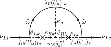
(c)

Figure 3: The contributions to the neutrino mass generations. A type of a diagram (a) is the corresponding diagram to the non-SUSY Zee-Babu model. Diagrams (b) and (c) are new type of diagram in the SUSY model.

It is non-trivial whether there is an allowed parameter region in our model except for the decoupling limit where masses of all the super partner particles are set to be much larger than the electroweak scale. Let us search for the parameter region where the neutrino mixing is consistent with the present oscillation data and the LFV constraints are satisfied.

Flavour violation in couplings between $\text{SU}(2)_{\text{L}}$ singlet fields and leptons should be large in order to generate large off-diagonal elements in the neutrino mass matrix. These large flavour violation couplings enhance the LFV processes. In particular doubly charged singlet scalar exchange tree level diagram contributes to the $e_{i}^{+}\to e_{j}^{+}e_{k}^{+}e_{l}^{-}$ process. The predicted decay width of $e_{i}^{+}\to e_{j}^{+}e_{k}^{+}e_{l}^{-}$ in the model is calculated asmacesanu ; aristizabal

$$\Gamma(e_{i}^{+}\to e_{j}^{+}e_{k}^{+}e_{l}^{-})=C_{jk}\frac{1}{8}\frac{(m_{e})_{i}^{5}}{192\pi^{3}}\left|(U_{\kappa})_{1a}^{*}(U_{\kappa})_{1a}\frac{g_{il}g_{jk}^{*}}{(m_{\kappa})_{a}^{2}}\right|^{2}\;,$$ (25)

where $C_{jk}$ is a statistical factor as

$$C_{jk}=\begin{cases}1&(j=k)\\ 2&(j\neq k)\end{cases}\;.$$ (26)

There can be still large contributions to $\mu\to e\gamma$, even if the constraint from $\mu^{+}\to e^{+}e^{+}e^{-}$ can be avoided. The contribution is from one-loop diagrams. The decay width of $e_{i}\to e_{j}\gamma$ is evaluated as

$$\Gamma(e_{i}\to e_{j}\gamma)=\frac{\alpha_{e}}{4}(m_{e})_{i}^{5}\left(|A_{L}^{ji}|^{2}+|A_{R}^{ji}|^{2}\right)\;,$$ (27)

with

$$A_{L}^{ji}= -\frac{1}{(4\pi)^{2}}\left\{(U_{\omega})_{1a}^{*}(U_{\omega})_{1a}\frac{4f_{kj}^{*}f_{ki}}{(m_{\omega})_{a}^{2}}F_{2}\left(\frac{(m_{\nu})_{k}^{2}}{(m_{\omega})_{a}^{2}}\right)-\frac{4f_{kj}^{*}f_{ki}}{(m_{\tilde{\nu}_{L}})_{k}^{2}}F_{1}\left(\frac{m_{\tilde{\omega}}^{2}}{(m_{\tilde{\nu}_{L}})_{k}^{2}}\right)\right\}\;,$$ (28)

$$A_{R}^{ji}= -\frac{1}{(4\pi)^{2}}\left\{(U_{\kappa})_{1a}^{*}(U_{\kappa})_{1a}\frac{g_{kj}^{*}g_{ki}}{(m_{\kappa})_{a}^{2}}\left(2F_{2}\left(\frac{(m_{e})_{k}^{2}}{(m_{\kappa})_{a}^{2}}\right)+F_{1}\left(\frac{(m_{e})_{k}^{2}}{(m_{\kappa})_{a}^{2}}\right)\right)\right.$$

$$\phantom{SpaceSpace}\left.-\frac{g_{kj}^{*}g_{ki}}{(m_{\tilde{e}_{R}})_{k}^{2}}\left(2F_{1}\left(\frac{m_{\tilde{\kappa}}^{2}}{(m_{\tilde{e}_{R}})_{k}^{2}}\right)+F_{2}\left(\frac{m_{\tilde{\kappa}}^{2}}{(m_{\tilde{e}_{R}})_{k}^{2}}\right)\right)\right\}\;,$$ (29)

where $(m_{\nu})_{i}$ are neutrino masses, and $(m_{\tilde{\nu}_{L}})_{i}$ are sneutrino masses. The loop functions $F_{1}(x)$ and $F_{2}(x)$ areinamilim

$$F_{1}(x)= \frac{x^{2}-5x-2}{12(x-1)^{3}}+\frac{x\ln x}{2(x-1)^{4}}\;,$$ (30)

$$F_{2}(x)= \frac{2x^{2}+5x-1}{12(x-1)^{3}}-\frac{x^{2}\ln x}{2(x-1)^{4}}\;.$$ (31)

The coupling constants $f_{ij}$ only have nonzero values in flavour off-diagonal elements, and they tend to be large to reproduce the bi-large mixing. Then the bound from the data becomes severe.

Let us discuss how the LFV processes constrain the parameter space. First of all, the tree level diagram contributing to the $\mu\to eee$ must be suppressed. The present bound on the branching fraction is $B(\mu^{+}\to e^{+}e^{+}e^{-})<1.0\times 10^{-12}$Bellgardt:1987du , which gives very strong constraint on the model parameter space. There are two possible cases to suppress the tree level contribution to the $\mu^{+}\to e^{+}e^{+}e^{-}$. The first possibility is considering heavy doubly charged bosons $\kappa_{1}$ and $\kappa_{2}$. If $g_{11}\sim g_{12}\sim 0.1$ is taken, the doubly charged bosons should be heavier than 15 TeV to avoid too large contribution. The second option is suppressing a product of the couplings $|g_{12}g_{11}|$. When the doubly charged bosons are $500$ GeV, the upper bound on the product $|g_{12}g_{11}|$ is obtained as $|g_{12}g_{11}|<10^{-5}$. The contributions to $\tau^{+}\to e^{+}e^{+}e^{-}$, $\tau^{+}\to e^{+}e^{+}\mu^{-}$, $\tau^{+}\to\mu^{+}\mu^{+}e^{-}$, $\tau^{+}\to\mu^{+}\mu^{+}\mu^{-}$, $\tau^{+}\to\mu^{+}e^{+}e^{-}$, and $\tau^{+}\to e^{+}\mu^{+}\mu^{-}$ can be computed in the same manner. These flavour changing tau decays into three leptons are also enhanced in the model with tree level contributions. If future tau flavour experiments such as the high luminosity B factoriessuperB would discover a signal of such decays, it could support the model. In the phenomenological point of view, the scenario with a light doubly charged singlet scalar is attractive because the scenario with such a light exotic particle is testable at the LHC. Therefore we have searched for a solution with a suppressed $|g_{12}g_{11}|$ and we have found that the coupling $g_{11}$ can be taken to be so small that the tree level contribution to the $\mu^{+}\to e^{+}e^{+}e^{-}$ process is negligible with reproducing the neutrino oscillation data. In such a parameter space, the $B(\mu^{+}\to e^{+}e^{+}e^{-})$ is suppressed by the electromagnetic coupling constant compared with $B(\mu\to e\gamma)$, say $B(\mu^{+}\to e^{+}e^{+}e^{-})\sim\alpha_{e}B(\mu\to e\gamma)$ where the current upper limit is given by $B(\mu\to e\gamma)<1.2\times 10^{-11}$ muegamma . The $B(\mu^{+}\to e^{+}e^{+}e^{-})$ is below the experimental upper bound, if the constraint of $B(\mu\to e\gamma)$ is satisfied.

In our analysis below, we work in the limit of $B_{\omega}\mu_{\Omega}\to 0$ and $B_{\kappa}\mu_{K}\to 0$ for simplicity. If these terms are switched on, the mixings in the charged singlet scalar mass eigenstates take part in the neutrino mass generation. However these mixings do not change our main results. In this limit, the mixing matrices $U_{\omega}$ and $U_{\kappa}$ become the unit matrix, and only $\omega_{1}$ and $\kappa_{1}$ contribute to the neutrino mass matrix and the LFV. Below we simply write the relevant fields as $\omega\equiv\omega_{1}$ and $\kappa\equiv\kappa_{1}$, and their masses are written as $m_{\omega}\equiv(m_{\omega})_{1}$ and $m_{\kappa}\equiv(m_{\kappa})_{1}$.

Following the above strategy, we search for an allowed parameter set. An example of the allowed parameter sets is

$$f_{12}=f_{13}=\frac{f_{23}}{2}=3.7\times 10^{-2}\;,\quad$$

$$g_{11}\simeq 0\;,\quad g_{12}=4.8\times 10^{-7}\;,\quad g_{13}=2.1\times 10^{-7}\;,\quad$$

$$g_{22}=-0.13\;,\quad g_{23}=6.1\times 10^{-3}\;,\quad g_{33}=-4.6\times 10^{-4}\;,\quad$$

$$\tilde{g}_{ij}=g_{ij}\;,\quad\lambda_{a}=1.0\;,\quad\mu_{B}=500\;\text{GeV}\;,\quad\frac{X_{k}}{m_{S}}=1.0\;,$$

$$(m_{\tilde{e}_{L}})_{k}=(m_{\tilde{e}_{R}})_{k}=(m_{\tilde{\nu}_{L}})_{k}=m_{S}=1000\;\text{GeV}\;,\quad$$

$$m_{\omega}=600\;\text{GeV}\;,\quad m_{\tilde{\omega}}=600\;\text{GeV}\;,\quad m_{\kappa}=300\;\text{GeV}\;,\quad m_{\tilde{\kappa}}=200\;\text{GeV}\;,\quad$$

$$(m_{\omega})_{2}\gg m_{\omega}\;,\quad(m_{\kappa})_{2}\gg m_{\kappa}\;.$$ (32)

On this benchmark point, the neutrino masses and mixing angles are given as

$$\sin^{2}\theta_{12}=0.33\;,\quad\sin^{2}\theta_{23}=0.5\;,\quad\sin^{2}\theta_{13}=0.0\;,$$

$$\Delta m_{21}^{2}=7.6\times 10^{-5}\;\text{eV}^{2}\;,\quad|\Delta m_{31}^{2}|=2.5\times 10^{-3}\;\text{eV}^{2}\;,$$ (33)

which are completely consistent with the present neutrino data: the global data analysisSchwetz:2008er of the neutrino oscillation experiments provide $\sin^{2}\theta_{12}=0.318^{+0.019}_{-0.016}$, $\sin^{2}\theta_{23}=0.50^{+0.07}_{-0.06}$, $\sin^{2}\theta_{13}=0.013^{+0.013}_{-0.009}$, $\Delta m_{21}^{2}=(7.59^{+0.23}_{-0.18})\times 10^{-5}\;\text{eV}^{2}$, and $|\Delta m_{31}^{2}|=(2.40^{+0.12}_{-0.11})\times 10^{-3}\;\text{eV}^{2}$. Based on this benchmark point, our model predicts $B(\mu\to e\gamma)=1.1\times 10^{-11}$ and $B(\tau^{+}\to\mu^{+}\mu^{+}\mu^{-})=1.3\times 10^{-8}$, both of which are just below the present experimental bounds. Since the LFV is naturally enhanced in the model, the MEG experimentMEG , which is expected to achieve $B(\mu\to e\gamma)<10^{-13}$ in a few years, will cover very wide regions of the parameter space. Apart from the bench mark scenario, there can be other parameter sets where the neutrino data and LFV data are satisfied. However, we here do not discuss details for such a possibility. A more general survey of the parameter regions may be performed elsewheretmp .

We turn to discuss collider phenomenology in the model assuming the parameters of the benchmark scenario given in Eq. (32). In our model, the new $\text{SU}(2)_{\text{L}}$ charged singlet fields are introduced, which can be accessible at collider experiments such as the LHC unless they are too heavy. In particular, the existence of the doubly charged singlet scalar boson and its SUSY partner fermion (the doubly charged singlino) provides discriminative phenomenological signals. They are produced in pair ($\kappa^{++}\kappa^{--}$ or $\tilde{\kappa}^{++}\tilde{\kappa}^{--}$) and each doubly charged boson (fermion) can be observed as a same-sign dilepton event, which would be a clear signature. In this Letter, we focus on such events including doubly charged particles. For the benchmark point given in Eq. (32), almost all the $\kappa$ decays into the same-sign muon pair, $\kappa^{\pm\pm}\to\mu^{\pm}\mu^{\pm}$.

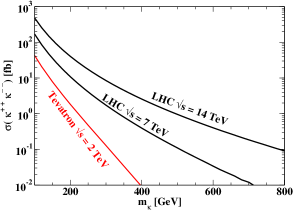
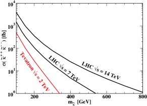
(a)		(b)

Figure 4: Production cross sections of (a) $\kappa^{++}\kappa^{--}$ and (b) $\tilde{\kappa}^{++}\tilde{\kappa}^{--}$, via Drell-Yan processes at the LHC ($pp$) and the Tevatron ($p\overline{p}$). The production cross section at the LHC is evaluated for $\sqrt{s}=7\;\text{TeV}$ and $\sqrt{s}=14\;\text{TeV}$.

At hadron colliders such as the LHC and the Tevatron, the doubly charged singlet scalar $\kappa$ and the doubly charged singlino $\tilde{\kappa}$ are produced dominantly in pair through the Drell-Yang processes. The production cross sections for $\kappa^{++}\kappa^{--}$ and $\tilde{\kappa}^{++}\tilde{\kappa}^{--}$ are shown as in Fig. 4(a) and Fig. 4(b), respectively. The first two plots from above correspond to the cross sections at the LHC of $\sqrt{s}=14$ TeV and $\sqrt{s}=7$ TeV, and the lowest one does to that at the Tevatron of $\sqrt{s}=2$ TeV. We note that magnitudes of the production cross sections for the pair of singly-charged singlet scalars $\omega^{+}\omega^{-}$ and that of singly-charged singlinos $\tilde{\omega}^{+}\tilde{\omega}^{-}$ are (1/4) smaller than those for $\kappa^{++}\kappa^{--}$ and $\tilde{\kappa}^{++}\tilde{\kappa}^{--}$ for the common mass for produced particles. The direct search of doubly charged Higgs bosons at the Tevatron gives the lower bound on the mass assuming large branching ratio decaying to muon pairs as $m_{\kappa}\gtrsim 150\;\text{GeV}$ :2008iy . Such a bound on the mass of doubly charged singlinos is partly discussed in Ref. singlino++ . At the LHC with $\sqrt{s}=7$ TeV with the integrated luminosity ${\cal L}$ of 1 fb^-1, about 100 of $\tilde{\kappa}^{++}\tilde{\kappa}^{--}$ pairs can be produced when $m_{\tilde{\kappa}}=200$ GeV, while only a couple of the $\kappa^{++}\kappa^{--}$ pair is expected for $m_{\kappa}=300$ GeV.

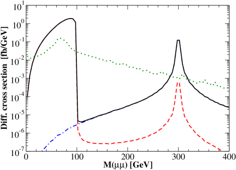
Figure 5: The invariant mass distribution of the same-sign dilepton event. The benchmark point in Eq. (32) is used and the neutralino mass is taken as $m_{\tilde{\chi}^{0}}=100\;\text{GeV}$. The dashed (red) curve corresponds to the events from $pp\to\tilde{\kappa}^{++}\tilde{\kappa}^{--}\to\tilde{\chi}^{0}\kappa_{1}^{++}\tilde{\chi}^{0}\kappa_{1}^{--}\to\tilde{\chi}^{0}\tilde{\chi}^{0}\mu^{+}\mu^{+}\mu^{-}\mu^{-}$. The dot-dashed (blue) curve shows the contributions from $pp\to\kappa^{++}\kappa^{--}\to\mu^{+}\mu^{+}\mu^{-}\mu^{-}$. The solid (black) curve denotes total events from the both signal processes. The dotted (green) curve shows the background events. For kinematical cut, see the text.

In Fig. 5, the distribution of the differential cross section for four muon (plus a missing transverse momentum) final states as a function of the invariant mass $M(\mu^{+}\mu^{+})$ of the same-sign muon pair is shown assuming the bench mark scenario in Eq. (32) at the LHC with $\sqrt{s}=7$ TeV. In order to suppress background events, we select the muon events with the transverse momentum larger than 20 GeV and the pseudo-rapidity less than 2.5. The signal events come from both $pp\to\kappa^{++}\kappa^{--}\to\mu^{+}\mu^{+}\mu^{-}\mu^{-}$ and $pp\to\tilde{\kappa}^{++}\tilde{\kappa}^{--}\to\tilde{\chi}^{0}\kappa_{1}^{++}\tilde{\chi}^{0}\kappa_{1}^{--}\to\tilde{\chi}^{0}\tilde{\chi}^{0}\mu^{+}\mu^{+}\mu^{-}\mu^{-}$. The $M(\mu^{+}\mu^{+})$ distribution can be a key to explore the phenomena with the doubly charged particles. The doubly charged scalar mass and the mass difference between the doubly charged singlino and the neutralino are simultaneously determined at the LHC. A sharp peak is expected in the $M(\mu^{+}\mu^{+})$ distribution at $M(\mu^{+}\mu^{+})=m_{\kappa}$, because the same-sign muon pair from the $\kappa$ decay is not associated with missing particles. On the other hand, the doubly charged singlino decays as $\tilde{\kappa}^{--}\to\tilde{\chi}^{0}\kappa^{--}\to\tilde{\chi}^{0}\mu^{-}\mu^{-}$ in the case that the lightest R-parity odd particle is a neutralino, $\tilde{\chi}^{0}$, which is a DM candidate in the model. In this Letter, we just assume that the LSP neutralino is Bino-like. In our analysis, we fix the neutralino mass as $m_{\tilde{\chi}^{0}}=100\;\text{GeV}$. The mass difference between $\tilde{\kappa}$ and $\tilde{\chi}^{0}$ can be measured by looking at a kink at $M(\mu^{+}\mu^{+})=m_{\tilde{\kappa}}-m_{\tilde{\chi}^{0}}$ in the $M(\mu^{+}\mu^{+})$ distribution. The main background comes from four muon events from the SM processes where muons are produced via the $ZZ$, $\gamma\gamma$ and $\gamma Z$ production, or a pair production of muons with the $Z$ or $\gamma$ emission. The expected background is also shown in Fig. 5. The events from signal dominate those from the background in the area of $M(\mu^{+}\mu^{+})<m_{\tilde{\kappa}}-m_{\tilde{\chi}^{0}}$ and at around $M(\mu^{+}\mu^{+})\sim m_{\kappa}$. The background events have been evaluated by using CalcHEPcalchep . From this rough evaluation, one may expect that the event from the signal can be identified even at the LHC with $\sqrt{s}=7$ TeV and ${\cal L}=1$ fb^-1. As for the case with $\sqrt{s}=14\,\text{TeV}$, the signal to background ratio becomes larger and it will be more promising to explore our model.

There are other models in which the same-sign dilepton events are predicted. The model with the complex triplet scalar fields is an example of such a class of modelstriplet . They can in principle be distinguished by looking at the decay products from doubly charged fields. In our scenario, $\kappa^{\pm\pm}$ can mainly decay into $\mu^{\pm}\mu^{\pm}$, while in the triplet models where the decay of doubly charged singlet scalars are directly connected with the neutrino mass matrix, there is no solution where only the $\mu^{\pm}\mu^{\pm}$ mode can be dominant decay mode. The difference in such decay pattern can be used to discriminate our model from the triplet models.

In this Letter, we have not discussed details for DM physics in our model. Assuming the Bino-like LSP, we expect that our DM candidate can satisfy the constraints from the WMAP data for the DM abundance in a similar way to the case in the similar scenario in the MSSM. We still note that the existence of doubly and singly charged particles in our model may change the cross section of DM pair annihilation at the one loop level to some extent, so that they may affect the DM abundance. The detail is, however, beyond the scope of this Letter, which will be discussed elsewheretmp .

We also give a comment on the possibility for baryogenesis. There can be several possibilities to realise baryogenesis in our model, such as using the Affleck-Dine mechanismAD , low energy leptogenesisZBlepto , and electroweak baryogenesis (EWBG). In the scenario of EWBG, the electroweak phase transition must be of strongly first order. In the MSSM the scenario of EWBG turns out to be rather challenging ewbg-mssm2 . On the contrary in our model, such a scenario may be natural and realistic. In our model, there are doubly and singly charged singlet scalar fields. When they have non-decoupling propertynondec ; Aoki:2008av ; aks_dm , the parameter region of the strong first order phase transition can be much wider than that in the MSSM. In addition, there can be many CP violating phases in the model, which are also required for successful baryogenesis.

We have discussed the SUSY extension of the Zee-Babu model under R-parity conservation. In the model, it is not necessary to introduce very high energy scale as compared to the TeV scale, and the model lies in the reach of the collider experiments and the flavour measurements. We have found that the neutrino data can be reproduced with satisfying the current bounds from the LFV even in the scenario where not all the superpartner particles are heavy. The LSP can be a DM candidate. Phenomenology of doubly charged singlet fields has also been discussed at the LHC.

The work of MA was supported in part by Grant-in-Aid for Young Scientists (B) no. 22740137, that of SK was supported in part by Grant-in-Aid for Scientific Research (A) no. 22244031 and (C) no. 19540277, and that of TS was supported in part by Grant-in-Aid for Scientific Research on Priority Areas, no. 22011007. The work of KY was supported by Japan Society for the Promotion of Science (JSPS Fellow (DC2)).

References

(1) P. Minkowski,
Phys. Lett. B 67 (1977) 421;
M. Gell-Mann, P. Ramond, and R. Slansky
in Supergravity, p. 315, edited by F. Nieuwenhuizen
and D. Friedman, North Holland, Amsterdam, 1979;
T. Yanagida,
Proc. of the Workshop on Unified Theories and the Baryon Number of the Universe, edited by O. Sawada and A. Sugamoto, KEK, Japan 1979;
Prog. Theor. Phys. 64 (1980) 1103;
S. L. Glashow,
in Proc. of the Cargése Summer Institute on Quarks and Leptons,
Cargése, July 9-29, 1979,
eds. M. Lévy et al. , (Plenum, 1980, New York), p707;
R. N. Mohapatra and G. Senjanovic,
Phys. Rev. Lett. 44, (1980) 912.
(2) J. Schechter and J. W. F. Valle,
Phys. Rev. D 22 (1980) 2227;
T. P. Cheng and L. F. Li,
Phys. Rev. D 22 (1980) 2860;
M. Magg and C. Wetterich,
Phys. Lett. B 94 (1980) 61;
C. Wetterich,
Nucl. Phys. B 187 (1981) 343;
G. Lazarides, Q. Shafi and C. Wetterich,
Nucl. Phys. B 181 (1981) 287;
R. N. Mohapatra and G. Senjanovic,
Phys. Rev. D 23 (1981) 165.
(3) R. Foot, H. Lew, X. G. He and G. C. Joshi,
Z. Phys. C 44 (1989) 441;
E. Ma,
Phys. Rev. Lett. 81 (1998) 1171.
(4) A. Zee,
Phys. Lett. B 93 (1980) 389
[Erratum-ibid. B 95 (1980) 461];
A. Zee,
Phys. Lett. B 161 (1985) 141.
(5)
A. Zee,
Nucl. Phys. B 264 (1986) 99.
(6)
K. S. Babu,
Phys. Lett. B 203 (1988) 132.
(7)
L. M. Krauss, S. Nasri and M. Trodden,
Phys. Rev. D 67 (2003) 085002.
(8)
E. Ma,
Phys. Rev. D 73 (2006) 077301.
(9)
M. Aoki, S. Kanemura and O. Seto,
Phys. Rev. Lett. 102 (2009) 051805.
(10) S. T. Petcov,
Phys. Lett. B 115 (1982) 401;
S. Kanemura, T. Kasai, G. L. Lin, Y. Okada, J. J. Tseng and C. P. Yuan,
Phys. Rev. D 64 (2001) 053007.
(11)
C. Jarlskog, M. Matsuda, S. Skadhauge and M. Tanimoto,
Phys. Lett. B 449 (1999) 240;
P. H. Frampton and S. L. Glashow,
Phys. Lett. B 461 (1999) 95;
Y. Koide,
Phys. Rev. D 64 (2001) 077301;
N. Haba, K. Hamaguchi and T. Suzuki,
Phys. Lett. B 519 (2001) 243;
X. G. He,
Eur. Phys. J. C 34 (2004) 371.
(12)
P. H. Frampton, M. C. Oh and T. Yoshikawa,
Phys. Rev. D 65 (2002) 073014;
K. Hasegawa, C. S. Lim and K. Ogure,
Phys. Rev. D 68 (2003) 053006.
(13)
K. S. Babu and C. Macesanu,
Phys. Rev. D 67 (2003) 073010.
(14)
D. Aristizabal Sierra and M. Hirsch,
JHEP 0612 (2006) 052.
(15)
M. Nebot, J. F. Oliver, D. Palao and A. Santamaria,
Phys. Rev. D 77 (2008) 093013.
(16)
T. Ohlsson, T. Schwetz and H. Zhang,
Phys. Lett. B 681 (2009) 269.
(17)
M. Aoki and S. Kanemura,
Phys. Lett. B 689 (2010) 28.
(18)
E. Komatsu et al.,
arXiv:1001.4538 [astro-ph.CO].
(19)
K. Cheung and O. Seto,
Phys. Rev. D 69 (2004) 113009;
K. Cheung, P. Y. Tseng and T. C. Yuan,
Phys. Lett. B 678 (2009) 293.
(20)
J. Kubo, E. Ma and D. Suematsu,
Phys. Lett. B 642 (2006) 18;
T. Hambye, K. Kannike, E. Ma and M. Raidal,
Phys. Rev. D 75 (2007) 095003;
D. Aristizabal Sierra, J. Kubo, D. Restrepo, D. Suematsu and O. Zapata,
Phys. Rev. D 79 (2009) 013011;
D. Suematsu, T. Toma and T. Yoshida,
Phys. Rev. D 79 (2009) 093004.
(21)
M. Aoki, S. Kanemura and O. Seto,
Phys. Rev. D 80 (2009) 033007;
M. Aoki, S. Kanemura and O. Seto,
Phys. Lett. B 685 (2010) 313.
(22)
J. van der Bij and M. J. G. Veltman,
Nucl. Phys. B 231 (1984) 205;
K. L. McDonald and B. H. J. McKellar,
arXiv:hep-ph/0309270.
(23)
T. Schwetz, M. A. Tortola and J. W. F. Valle,
New J. Phys. 10 (2008) 113011.
(24)
P. G. Camara, L. E. Ibanez and A. M. Uranga,
Nucl. Phys. B 689 (2004) 195.
(25)
L. J. Hall and L. Randall,
Phys. Rev. Lett. 65 (1990) 2939.
(26)
I. Jack, D. R. T. Jones and A. F. Kord,
Phys. Lett. B 588 (2004) 127.
(27)
M. Aoki, S. Kanemura, T. Shindou, and K. Yagyu, in preparation.
(28)
T. Inami and C. S. Lim,
Prog. Theor. Phys. 65 (1981) 297
[Erratum-ibid. 65 (1981) 1772].
(29)
T. Aushev et al.,
arXiv:1002.5012 [hep-ex];
M. Bona et al.,
arXiv:0709.0451 [hep-ex].
(30)
M. L. Brooks et al. [MEGA Collaboration],
Phys. Rev. Lett. 83 (1999) 1521.
(31)
U. Bellgardt et al. [SINDRUM Collaboration],
Nucl. Phys. B 299 (1988) 1.
(32)
V. M. Abazov et al. [D0 Collaboration],
Phys. Rev. Lett. 101 (2008) 071803;
T. Aaltonen et al. [The CDF Collaboration],
Phys. Rev. Lett. 101 (2008) 121801.
(33) B. Dutta, R. N. Mohapatra and D. J. Muller,
Phys. Rev. D 60 (1999) 095005;
M. Frank, K. Huitu and S. K. Rai,
Phys. Rev. D 77 (2008) 015006;
D. A. Demir, M. Frank, D. K. Ghosh, K. Huitu, S. K. Rai and I. Turan,
Phys. Rev. D 79 (2009) 095006.
(34)
E. J. Chun, K. Y. Lee and S. C. Park,
Phys. Lett. B 566 (2003) 142;
M. Kakizaki, Y. Ogura and F. Shima,
Phys. Lett. B 566 (2003) 210;
A. G. Akeroyd and M. Aoki,
Phys. Rev. D 72 (2005) 035011;
J. Garayoa and T. Schwetz,
JHEP 0803 (2008) 009;
A. G. Akeroyd, M. Aoki and H. Sugiyama,
Phys. Rev. D 77 (2008) 075010;
M. Kadastik, M. Raidal and L. Rebane,
Phys. Rev. D 77 (2008) 115023;
P. Fileviez Perez, T. Han, G. y. Huang, T. Li and K. Wang,
Phys. Rev. D 78 (2008) 015018.
(35)
T. Mori et al., Research Proposal to Paul Scherrer Institut (1999);
see also http://meg.web.psi.ch/
(36)
A. Pukhov et al.,
arXiv:hep-ph/9908288;
A. Pukhov,
arXiv:hep-ph/0412191.
(37)
I. Affleck and M. Dine,
Nucl. Phys. B 249 (1985) 361.
(38)
C. S. Chen, C. Q. Geng and D. V. Zhuridov,
arXiv:0806.2698 [hep-ph].
(39)
M. Carena, G. Nardini, M. Quiros and C. E. M. Wagner,
Nucl. Phys. B 812 (2009) 243;
K. Funakubo and E. Senaha,
Phys. Rev. D 79 (2009) 115024.
(40)
S. Kanemura, Y. Okada and E. Senaha,
Phys. Lett. B 606 (2005) 361.