Non-linear evolution in CCFM: The interplay between coherence and saturation
Abstract:
We solve the CCFM equation numerically in the presence of a boundary condition which effectively incorporates the non-linear dynamics. We retain the full dependence of the unintegrated gluon distribution on the coherence scale, and extract the saturation momentum. The resulting saturation scale is a function of both rapidity and the coherence momentum. In Deep Inelastic Scattering this will lead to a dependence of the saturation scale on the photon virtuality in addition to the usual dependence. At asymptotic energies the interplay between the perturbative non-linear physics, and that of the QCD coherence, leads to an interesting and novel dynamics where the saturation momentum itself eventually saturates. We also investigate various implementations of the ”non-Sudakov” form factor. It is shown that the non-linear dynamics leads to almost identical results for different form factors. Finally, different choices of the scale of the running coupling are analyzed and implications for the phenomenology are discussed.
1 Introduction
The linear QCD evolution equations at small-, such as BFKL [1] or CCFM [2, 3, 4, 5, 6], lead to a very rapid growth of the gluon density. Once the density is too large however, one needs to take into account the non-linear effects. The BFKL evolution is modified in the high density limit by the so-called Color Glass Condensate (CGC) [7, 8] (for a review see [9]) formalism where the strong color fields are treated semi–classically, and where their presence leads to the saturation of the gluon emission rate111This implies that the gluon density keeps growing also in the saturated regime but the growth is logarithmic in as opposed to power-like.. The BFKL evolution equation is then generalized to either the Balitsky-Kovchegov (BK) [10, 11] equation or to the more complete JIMWLK [12, 13] equation. The energy dependent momentum scale characterizing the transition from the weak to strong field regimes is called the saturation momentum and is denoted .
What makes CCFM different from the standard BFKL-type picture of the small- regime is the property of the so-called coherence of emissions. This is quantum mechanical in origin and comes from the interference in the emission of gluons from different partons. This leads to what is termed angular ordering which, as a fundamental feature of QCD, is present in both time-like and space-like evolution as well as at both small and large . In CCFM the effects of angular ordering are encoded in an additional momentum scale, usually denoted , so that the unintegrated gluon density now depends on three variables: Bjorken , the momentum , and the additional momentum . We will denote the unintegrated gluon density by . In comparison, the BFKL gluon density, and similarly the density in the CGC formalism, depends only on and , that is .
The saturation scale is the momentum at which the gluons in the hadron start to overlap with each other. This leads to the increased rate for the recombination of gluons. can be defined as the momentum for which is a given constant, say of the order of 1. This is a natural definition since the gluon density can be defined as a phase space occupation number222 The exact relation between and the occupation number depends on the precise definition of the former. of gluons per unit rapidity with given transverse momentum . This automatically implies that is dependent. However, it is then clear that in CCFM the same definition immediately leads to an extra scale dependence of , since now the requirement of constant occupation number, , leads to . One of our main objectives in this paper is to study this novel scale dependence of by numerically solving the CCFM equation in the presence of a boundary condition enforcing non-linear corrections.
The additional momentum variable in CCFM is determined by the kinematics of the hard scattering. More precisely, the hard scattering determines the maximal angle of the allowed emissions in accordance with angular ordering. Conventionally one uses the squared angle as the angular variable, and for example in a DIS process with gluon emissions, angular ordering implies that where is the maximal angle determined by the hard scattering. The transverse momentum is then defined via where is the energy fraction of the gluon entering the hard scattering, and is the cms energy. The variable is related to in DIS, roughly . This means that the saturation scale from CCFM in DIS kinematics will depend on the photon virtuality in addition to the Bjorken . In the usual picture of the small- physics, however, is an intrinsic property of the target hadron, and is independent of the probe and its virtuality. The difference now is that the gluon occupation number in the hadron depends additionally on the probe. That is not a property of the target alone but also depends on the probe and its virtuality is certainly what one would generally expect from quantum mechanics. In the end is determined by the scattering process, to which both the probe and the target enters, and therefore we should expect to depend on both. In that sense the extra scale dependence of is most natural.
Unlike BFKL, the proper non-linear generalization of CCFM is not know yet, and we shall not present it here either. In [14, 15], however, a method was proposed which effectively implements saturation and unitarity corrections within a generic linear evolution equation, and the method was in particular applied to BFKL and CCFM. The idea is simply based on enforcing a boundary condition in the linear evolution which prevents the gluon phase–space occupation numbers to grow too large, and the procedure is an extension of a strategy originally introduced in connection with analytic studies of BFKL evolution in the presence of saturation effects [16, 17]. The method was demonstrated to work very well for BFKL in [14] where the solutions of BFKL in the presence of the saturation boundary condition were compared to the solutions of BK, and it was shown that the method reproduces successfully the results from BK for any and for both fixed and running .
The method was then applied to CCFM in [15] and was extracted. However, in order to simplify the numerical procedure, only the case was studied in which case one can neglect the dependence on so that depends only on . This is the region that leads to another formulation of CCFM called the Linked Dipole Chain (LDC) model [18] which has some advantages compared to CCFM such as projectile-target symmetry. In this paper, we will keep the full dependence of the evolution, and we will show that this dependence, which as mentioned above is related to coherence in the emissions, combined with the physics of saturation gives rise to a very interesting and novel dynamics which eventually leads to the saturation of the saturation momentum itself. This happens when the solution to ”stalls” in some region of , meaning that the evolution in is almost completely stopped. This behavior is in contrast to the standard picture of the non-linear dynamics where grows indefinitely with .
Generally we shall see that the shape of and that of close to the saturation regime is in CCFM rather different than in BFKL. Also some characteristic features of the standard small- evolution such as geometric scaling [19] is modified in CCFM. On the practical level, however, it seems that the new behavior of , whereby it eventually saturates as a function of for given , sets in very late, especially with a running coupling, so that it seems it would be be very hard to observe at collider experiments. On the other hand it will still be important to take into account the variation of with also for phenomenological values of , especially when is small.
In this study, we restrict ourselves to the version of CCFM containing only the ”hard” emissions associated with the pole in the gluon splitting function. In addition to these, in CCFM there are also the ”soft” emissions which are associated with the opposite pole333In addition to the singular pieces of the splitting function, the non-singular pieces are usually included in phenomenological applications, such as in the CASCADE Monte Carlo [20]. While these terms may obviously be important in practice it should be noted that their inclusion is somewhat ad hoc since they were not properly included in the original formulation of CCFM.. Within the accuracy of the formulation of CCFM however, these emissions are exactly ”probability conserving”, meaning that they are exactly compensated by the associated virtual corrections encoded in the so-called ”Sudakov” form factor. Thus at least formally, it should make no difference for the solution of whether one includes the soft emissions or not. The difference would be only in the exclusive final state, a correct description of which requires the soft emissions. In practice, however, such a formal statement carries little significance, and the inclusion of soft emissions can have substantial effects on . Thus it is our aim to also include the soft emissions in our procedure. This is, however, somewhat challenging numerically due to the fact that the real and virtual terms are separately divergent, and so one must introduce a cut-off which complicates the numerical procedure. Therefore the inclusion of the potentially important soft emissions and the associated Sudakov form factor is postponed to a future work.
The emissions are accompanied by virtual corrections which are encoded in the so-called ”non-Sudakov” form factor. One can in the literature find different expressions for this form factor. In this paper we shall study both of the common expressions for the form factor. We shall see that, generally, the different choices of the non-Sudakov form factors lead to rather different results in the linear evolution, which is due to the reason that the differences which occur in the softer region are enhanced unless there is some mechanism to cut off the growth there. As we will demonstrate, once non-linear evolution is included via the saturation boundary condition, then the differences are to a large degree removed. The small differences remaining when is extended to very large values can can be removed by scale factors independent of and . Thus saturation introduces a certain universality in the evolution as was already observed in [15].
Related to this, it is important to check the sensitivity of the results to different prescriptions of the boundary condition. Generally, one can consider different boundary conditions or, for a given type of boundary, different values of the boundary parameters. In [15] it was reported that the different choices lead to different normalizations of the solutions, without altering the shape or the dependence. Since we here keep the dependence, the question is more subtle. We will show that the differences are small and that they can generally be removed by and independent scale factors. Some differences can remain in the region where starts to saturate (the region where ”stalls”), but what we find is that this behavior itself, i.e the saturation of , is independent of the precise application of the boundary. What changes is simply at what , for a given , this behavior sets in. To know the exact details of the behavior in the saturated regime one would need to fully formulate the proper non-linear generalization of CCFM which is beyond the scope of this work. It seems, however, rather reasonable to expect that this interesting dynamics where, as a result of the combination of saturation and coherence, eventually saturates will remain true also once the proper non-linear generalization of CCFM is known.
The structure of the paper is the following: in the next section we present a brief overview of the CCFM formalism and show the numerical results for the solution in the case when the full dependence on the scale is included. We also discuss different versions of the running coupling prescriptions. In section 3 we provide semi-analytical results for the case of CCFM with the boundary condition. In particular, we discuss the dependence of the saturation scale on the rapidity and . In section 4 we briefly describe the method of implementation of the saturation boundary. In section 5 we present the complete numerical analysis of CCFM in the presence of the saturation boundary. We analyze different prescriptions for the non-Sudakov form factors and the running coupling, and we extract the rapidity and dependence of the saturation scale. Finally, in section 6 we state our conclusions and discuss the relevance of the results for the phenomenology.
2 Overview of CCFM
Our aim in this section is to provide a brief overview of CCFM, focusing on the points which shall be relevant for our analysis. It is possible to find different versions of the non-Sudakov form factor in the literature but the origin of this form factor is hardly ever discussed. It will therefore be important to recall the derivation of this form factor and understand the motivation behind the formulas. Moreover, we shall in addition to the standard choice of the scale of the running coupling also consider a different choice. The most comprehensive overview is to be found in the original papers in [2, 3, 4, 5, 6], and a simplified but rather detailed discussion on CCFM is also offered in [15].
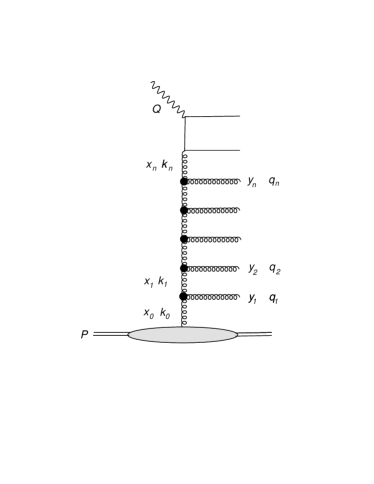
The gluon ladder generated by the CCFM evolution is represented in figure 1. In CCFM the successive emissions along the ladder are ordered in their angle. As mentioned in the introduction, it is customary to define as the angular variable (with the direction of the incoming proton defining the longitudinal direction), and angular ordering implies that . Additionally there is a maximum angle , set by the kinematics of the hard scattering, which limits all emissions.
In CCFM, the emissions are divided into hard and soft emissions, and the importance of this classification is that it offers significant simplifications in the formulation. The precise definition is that the hard emissions are those emissions ordered in both energy and angle, while for each soft emission there exists another emission with bigger angle and larger energy fraction. It follows that, the hard emissions are those associated with the pole in the gluon splitting function while the soft emissions are associated with the opposite pole. Following the above definition one can associate with each hard emission a cluster of soft emissions which satisfy and where is the angle of the previous hard emission. The label ”soft” has a two-fold meaning. Firstly the fact that each of these emissions takes away very little energy, because of the pole, and secondly that all soft emissions in the set satisfy . The classification of the emissions as being hard or soft is also related to another classification of the ladder in terms of so-called –changing and –conserving emissions respectively. What is meant by this is that there are certain real emissions which leave the virtual propagator momenta unchanged in an approximate sense. This latter classification is crucial for deriving the ’standard’ version of CCFM which is used in all practical applications.
2.1 Integral equations and the virtual form factors
The CCFM integral equation, including both the soft and the hard emissions, is given by
| (2.1) |
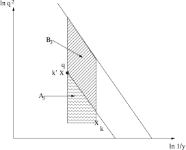
The momentum variable is defined via , and . The momentum is the rescaled momentum of the real gluon, and is related to the true momentum by . In line with all the approximations made in order to derive this equation one can for the pole set (which is what we have already done in ). Here is the Sudakov form factor which screens the singularity of the pole, while is the ”non-Sudakov” form factor which depends also on the momenta and it corresponds in BFKL to the gluon Regge factor. The rescaled coupling constant is defined as .
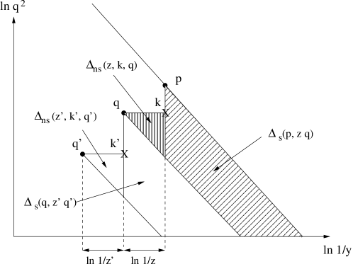
In figure 2 we represent pictorially the components of equation (2.1). Here the horizontal axis represents the inverse energy fraction of the gluons, the further to the right a gluon is located the less energy it has, while the vertical axis represents the transverse momenta, the higher up a emission is located the larger its transverse momentum. The maximal angle is represented by drawing a line of constant angle from the point ; this is the diagonal line going through the black dot representing ( itself is not the momentum of any gluon (real or virtual) but we still denote its location by a dot in the figure). In this particular case, . The ”Sudakov” form factor is then given by exp where is the phase space area which is the diagonally shaded region in the figure. This is the region where further emissions would have been possible. Similarly the ”non-Sudakov” form factor is given by exp where is the area of the vertically shaded region. In the figure we also show the next backward step in the evolution which is obtained from (2.1) when in the RHS is expanded iteratively. As we can see from the figure, the region contributing to diverges when extended down indefinitely. Thus this divergence is cut by a horizontal line in the figure, which means a soft cut-off in the transverse momentum. Notice that this divergence is the one arising from the pole because as , the gluon carries infinitely small energy fraction, and in the figure it would then be located precisely in the region where the diagonally shaded region is extended down indefinitely (the fact that this region is bounded by the diagonal lines is due to angular ordering).
The soft emissions are such that they are exactly compensated by the factors . This means that the regions over which the Sudakov form factors receive contribution are precisely the regions to which the soft emissions are confined, i.e. the clusters mentioned above. Summation over all possible soft emissions in each leads to a factor exp. Each such factor then multiplies to unity with the corresponding Sudakov form factor exp. One is consequently left with the hard emissions only, and the integral equation reads
| (2.2) |
This equation is thus formally equivalent to (2.1). In practice, however, one can expect to find different solutions. The numerical implementation of the soft emissions faces the difficulty that one must cut the singularity by a momentum cut-off as in figure 2. This introduces a numerical uncertainty which complicates the procedure. Therefore, even though their inclusion is important and interesting, we will postpone their treatment to a future work and in the present concentrate only on equation (2.2).
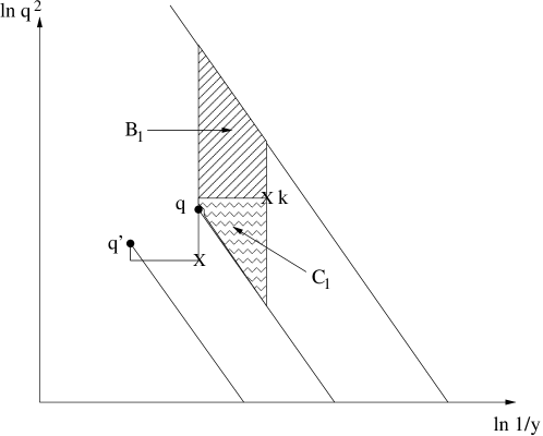
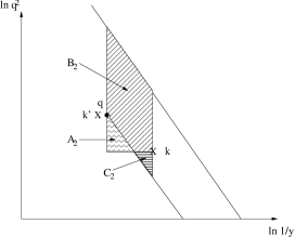
As mentioned above, the non-Sudakov form factor can be written as exp, where in figure 2, is the vertically dashed region bounded by and the angle of , and the energies of and . In CCFM, the form factors and are derived out of the so-called eikonal, , and non-eikonal, , form factors which sum up to all orders the virtual corrections associated with the eikonal and non-eikonal emission vertices respectively [2, 3, 4, 5, 6]. As shown in [15], for each emission the product of the associated form factors and equals the BFKL form factor , that is . The definition of for a given emission is that it is the product between and a portion of the eikonal form factor which covers a region bounded from below by the angle of and from above by the maximal angle (this is the region left over after multiplication with a soft factor coming from the resummed real emissions). In figure 3 this is the sum of the shaded regions and . The non-eikonal form factor itself is such that it covers a region bounded from below by while from above it is again bounded by , this is region in the same figure. What is important however is that the sign in the exponential factor is reversed, so that it is positive.444This actually comes from the fact that contains virtual corrections which are generated by the product between the non-eikonal current and the eikonal current , while is generated by the square of the eikonal current . This leads to a sign difference between the form factors, for details see [2, 3, 4, 5, 6]. The non-Sudakov is then given by
| (2.3) |
In this case, however, we assumed that , see figure 3. Now, if we can have two different situations, depending on whether or not is entirely below the diagonal line through in the figure, that is whether or . In these both cases we define a new region shown in figure 4. This is a region bounded from below by and from above by the angle of . When as in figure 3 of course .
On the left plot of figure 4 we show the case when , and the definition of then yields
| (2.4) |
If is bigger than then we see that is larger than unity. In case we instead have (in this case )
| (2.5) |
Thus exceeds unity when , and this actually happens when . All the results above give
| (2.6) |
Therefore if the kinematical constraint is assumed to be valid, is guaranteed to be bounded by unity555In that case , despite its name, works as a Sudakov and it can be used to cancel the -conserving hard emissions. One is then left with a much simplified formula. This was first understood and used in [18], and it was used in the analysis in [15] as well. . A different version of was presented in [21] in which case the regions are simply neglected. Then one always has
| (2.7) |
where
| (2.8) |
Since is neglected, we are thus guaranteed that . Thus in a sense this
has a similar effect to assuming the kinematical constraint to hold, but one should still keep
in mind that the effect is not the same because one has no apparent reason to simply
neglect the regions (this amounts to neglecting soft emissions above , see
also discussion below). What the kinematical constraint ensures is that .
In this paper, we will not include the kinematical constraint (it was included in [15]), which must be included
in the real emissions as well, but we shall rather
study the differences between using the two different non-Sudakov form factors,
(2.6) and (2.7).
2.2 Scale of the running coupling
Above we assumed a fixed coupling which is consistent with formulation of CCFM which was only performed at LO where the coupling is fixed. Although the effects of the running coupling are formally of next to leading order, it is nevertheless for any phenomenological application extremely important to take into account the running of the coupling.
The standard procedure is to let the coupling run with in the pole and in which is similar to what is usually done in LO BFKL. When both hard and soft emissions are included then is usually chosen as the relevant scale for in the pole and in (this is for example done in CASCADE as well as in the SMALLX program [22]). Notice that multiplies also the pole so with this choice one is for the hard emissions using as scale for the Sudakov form factor while is used for the non-Sudakov and the real emissions.
As is the larger scale in it may seem natural that it is chosen as the scale for the running coupling. However, once a scale is chosen for a certain class of emissions, say the hard emissions, then that scale should be consistently applied everywhere because otherwise some cancelations which are important for the consistency of the formalism may be violated. Also, even though seems to be the larger scale in we have seen above that actually in the derivation of , first enters as the lower scale in .
In [22] it is argued that the choice to have and as scales simultaneously can be derived from having the single choice (where is now the four momentum squared), since this choice reduces to and when and respectively. One should, however, again remember that both and are derived out of and , and while the four momentum of could be argued as scale in the latter, the former resums the graphs where virtual gluons are emitted and absorbed in between the real gluons so it is hard to see why the scale of should also be used here. We find it more plausible that instead the momenta of the virtual gluons are used in . But if this choice is made, then to derive and in the first place, one has to choose as scale in too, since otherwise necessary cancelations between and would not work. Consequently this leads to using in both and , and therefore also in all the real emissions.
If one uses as scale in then obviously the formula in (2.6), and similarly the corresponding one in (2.7) is the same as in the fixed coupling case. If on the other hand one uses the virtual momentum as scale for , then the formula is changed. We use as scale in (2.7) and derive a new formula which is however somewhat lengthy so we do not present it explicitly. We shall use the one loop result for the running coupling, frozen below some scale ,
| (2.9) |
Thus for the running coupling case we shall consider the following alternatives: One in which we use as scale and given in (2.6), one in which we use as scale and in (2.7), and the last case where is chosen as scale in and the corresponding modified is used.
We shall note here that, in the BFKL equation the coupling also starts to run at the next-to-leading logarithmic level (in ) only [23, 24, 25, 26, 27, 28]. The different choices of scales formally lead to the differences at next-to-next-to leading level. They are however not negligible numerically. The form of the NLL correction suggests that the most natural scale is that of the transverse momentum squared of the emitted gluon, see for example [29, 30]. This confirms the choice of (2.9) as a more natural choice of scale.
2.3 Numerical results for the linear case
2.3.1 Different versions of the non-Sudakov form factor
We will present here numerical results for the solution to the linear CCFM evolution. We start with the comparison of the two versions of the non-Sudakov form factor (2.6) and (2.7) in the case when the coupling is fixed, and set to be equal to . In figure 5 we present the value of the unintegrated gluon distribution obtained from CCFM as a function of the transverse momentum , and for the fixed value of the momentum (left plot) and (right plot). Different curves in increasing order correspond to increasing values of the rapidity. The initial condition for the equation was set to be
| (2.10) |
with . It is clear that the ’non-regular’ form-factor given by (2.6) gives a significant contribution in the low momentum regime due to the fact that so that the expression in the exponent changes sign. This gives a substantial enhancement at low values of . On the other hand it is also clear that both prescriptions for the form-factors coincide in the large regime. One observes that the slope of the distribution becomes steeper when becomes larger than , meaning a suppression of the momenta due to angular ordering. Momenta larger than are nevertheless allowed. This change in the slope in is crucial for the analysis with the boundary and the behavior of the saturation scale as we shall see later.
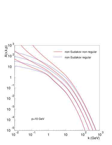
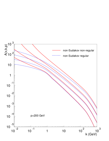
2.3.2 Fixed vs running coupling
In figure 6 we perform the comparison between the running and fixed coupling scenarios. The running coupling is regularized at with frozen scenario. As expected the running coupling gives the higher contribution in the region of the infrared momenta. It falls then below the fixed coupling at high momenta but such that , as the running coupling value becomes smaller than the fixed value . The effect is most pronounced for the calculation with . We observe though that in the region where , the scenario with the running coupling gives results which tend to be larger. One needs to take into account the fact that in this region we have stronger relative suppression from the non-Sudakov form-factor (we shall discuss this more below). The value of the form-factor is smaller for the larger value of , which is for the case of the fixed coupling. This is why the running coupling calculation tends to be less suppressed in the asymptotic regime of the large transverse momenta.
2.3.3 Comparison between different versions of the running coupling
Next let us turn to the implementation of different scales in the running coupling. In figure 7 we show the comparison between the standard results and those obtained using as scale. The differences between two choices are in general not too large, with the choice of giving smaller values for the solution. In the case when there are more and more chains with contributing, and so typically . Therefore the solution with as a choice of the scale is slightly lower.
On the other hand, when is small () we see that the differences are larger, and especially the dependence and the slope of seem to be modified. In this regime the phase space is strongly constrained by the maximum angle allowed for the emissions. The phase space restriction applies to the real momenta , while the virtual momenta are not directly restricted. Then in an event where we would expect that generally as well (except early in the chain). This implies that and one could therefore expect to see a faster growth when is chosen as the scale. However, the opposite behavior is observed. This is because a larger coupling also implies that there is a larger suppression from . We saw a hint of this behavior already in figure 5. When the phase space for the real emissions is more strongly constrained, on the other hand (2.6) or (2.7) are independent of , so even if the real phase space is strongly constrained, the form-factor is not. This implies the possibility that a larger coupling in this regime actually slows down the evolution due to the large suppression from .
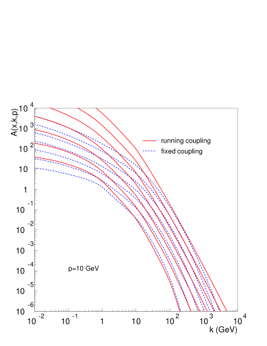
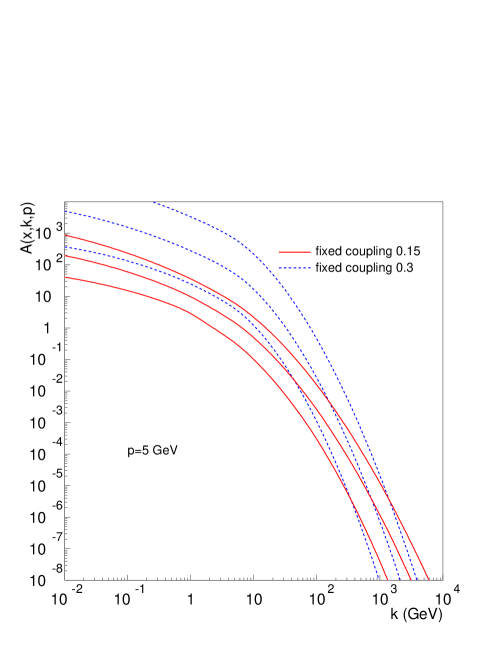
To further demonstrate that this is indeed the case we show in figure 8 results obtained from two different values of the fixed coupling, and , for GeV. For clarity of demonstration we show only solutions for . Of course in this case since for any , in the region where the solution with the larger coupling indeed grows faster (the phase space restriction is not so important here). However, we then clearly see that as , the suppression from , which is much larger when , starts to dominate and therefore the solution with the larger coupling is strongly suppressed. Consequently in the region , the solution with the larger coupling actually grows slower.
3 CCFM in the presence of saturation: analytical results
Having reviewed some of the basic concepts in CCFM we now move on to the question of implementing saturation effects and finding the relevant saturation scale . The implementation of saturation effects will be done using the same approach as in [14, 15], but most importantly because in this work we do keep the full dependence of on the additional scale , we shall discover many interesting new results not noticed before. The main implementation is numerical and all the numerical results are to be presented in section 5. In this section we will analytically study the general behavior of .
To study the saturation scale it is convenient to take the Mellin transform over the momentum . Following [31] we shall write the Mellin representation of as
| (3.11) |
where , and we define with an arbitrary scale. We will only consider the fixed coupling case in the analytic formulas. The function encodes the dependence of on the parameter . What we know generally is that when , since the restriction coming from becomes irrelevant in that case. This, however, does not imply that angular ordering is not important anymore. More precisely it means that the ordering in the final step of the evolution is automatic when , but in the previous steps of the evolution it is still important. This will reflect itself in the characteristic function which in the limit is given by
| (3.12) |
To find the function one can differentiate the integral equation (2.2) with respect to as done in [31]. One then finds that
| (3.13) |
where as before . Assuming that is very large and the solution is in the asymptotic region one can neglect the first theta function, which is what is done in [31]. However, one should then notice that with the non-Sudakov in (2.6) which is allowed to exceed unity, one would run into a divergence. This is so because when , even if is finite, the phase space for the emissions contributing to the scattering becomes infinitely large, and there is a UV divergence appearing when . On the other hand such a divergence does not appear if the restricted in (2.7) is used instead. The reason for this is that the choice in (2.7) effectively implies that plays the role of a UV cut (but only for the soft emissions). If the restriction from is removed (as when ) then the form factors and need to be regularized by some UV cut-off. When these factors are multiplied together, because of the different signs, they cancel each other in the region above , and thus the dependence on the UV cut-off vanishes. However, the real emissions need still be regularized by the UV cut-off, since otherwise the inclusive summation over the soft emissions for the given hard emission would give a divergence as . The fact that the regions in figures 3 and 4 are neglected in the derivation of (2.7) means that one is cutting off all real soft emissions above which is why plays the role of the UV regulator666At this point it should, however, be mentioned that there is no reason for the soft emissions to be bounded by . This would essentially be true if the soft emissions were conserving in the angular ordered cascade. The fact is that they are conserving, but not with respect to the angular ordering, but rather to the energy ordering whereby each emission is indexed according to its energy, and the ”propagator” momenta are defined accordingly. for the soft emissions. Thus for simplicity we shall use this form factor in the following, though a proper renormalization procedure for all the emissions would probably be called for.
After these remarks, let us now return to the equation for above.
The saturation of the solution can be analyzed in the two different regimes of large and small .
The case when :
In case , since (because of the theta function in (3.13)), we also have that . We will then approximate . Equation (3.13) is then easily solved to give
| (3.14) | |||||
where in the second equality we neglected the term exponential in , because it is very small when is large. We have also defined . Consistency of the solution requires that
| (3.15) |
We see that when , that is when is very large, reduces to unity. Since is large we can rewrite as
| (3.16) |
The Mellin representation then reads
| (3.17) |
To find the saturation scale, one can essentially follow a line of constant density [16, 17] which means that the relevant saddle point for the saturation problem is determined by the equations (defining )
| (3.18) | |||||
| (3.19) |
Here all derivatives are with respect to and the second equation is the usual saddle point condition while the first equation states that the integrand around the saturation scale is constant and of order 1. On the other hand we recall that in the saturation problem for BFKL the corresponding saddle point equations read
| (3.20) | |||
| (3.21) |
What we notice, besides the fact that the equations in CCFM look much more complicated than in BFKL, is that equations (3.18) and (3.19) imply that the saturation anomalous dimension , and thus also the characteristic function , depend generally on and . In BFKL on the other hand, is a pure number and is independent of which we see from the corresponding equations. As , we see that the structure of the CCFM saddle point equations reduce to the BFKL ones, though at finite , and are still different than in BFKL. When , the CCFM solution reduces completely to the BFKL one.
From equation (3.18) we can find . Let be the solution when , that is
| (3.22) |
Since the general form of which depends on is complicated, we will in the following simply make the approximations to set and . Then let us write777The minus sign in front of the correction term comes from the fact that a finite reduces the phase space and should therefore reduce too. , and we get
| (3.23) |
Since (it is suppressed by both and the exponential) we must have , and therefore
| (3.24) |
Thus we find that
| (3.25) |
which is valid as long as . The saturation saddle point is determined by
| (3.26) |
as in BFKL. Of course this is the lowest order approximation (lowest order with respect to the corrections in , but it is valid at finite ) but since the more general case is rather complicated we shall use this formula. In the later section we will determine the full saturation momentum via the numerical solution.
In order to be able to use the formula (3.25) one needs to have a solution for the characteristic function in CCFM. This is essential for obtaining and . Unfortunately it is only possible to extract the characteristic function numerically, as was done in [31]. To estimate here the dependence of the saturation scale on and from (3.25) we will use a simple model for the characteristic function,
| (3.27) |
This model corresponds to the LO BFKL equation with the kinematical constraint included. It is well known that it leads to the significantly reduced value of the intercept [32, 33] and thus it should be fairly close numerically to the CCFM characteristic function. One can extract and solving numerically equation (3.26). For the standard choice of the coupling constant we obtained , and . Using these extracted values we can determine saturation scale from the equation (3.25). We demonstrate the results in figure 9. The curves increasing are for different values of the momentum scale .
It is evident that for small rapidities the growth of the saturation scale is dominated by the term exponential in rapidity and the characteristics is similar to the BK equation (or BFKL with the saturation boundary). However for fixed value of scale the dependence of on rapidity becomes nonlinear. The smaller the value of is, the lower is the critical value of rapidity for which the behavior starts to become nonlinear, and there is an additional dependence on . The formula cannot be trusted in the region where falls off with rapidity. This region is outside the validity of the original approximation in which equation (3.25) was derived. One would need to compute higher order corrections and possibly resum them in order to predict the asymptotic behavior of with .
Thus the leading term for the saturation momentum when is very large has the same structure as in BFKL, with the ”speed”, , of being much slower, around for CCFM as opposed to around for BFKL at LO and . The corrections coming from finite slow down the saturation scale and from (3.25) we see that the dependence in enters as a power inside an exponential. Summarizing, we observe that the corrections from the phase space restriction in CCFM introduce an increasingly complicated shape of depending both on and when going beyond the BFKL regime, i.e. .
Using the results above one can also study the behavior of near saturation, that is when . This is done by expanding the function in the exponential of the Mellin representation to . In BFKL this leads to
| (3.28) |
The BFKL result features the well known characteristics of the small- evolution. One is the property of geometric scaling which is the fact that the and dependence enters the gluon distribution in the combination , that is via . Indeed as long as the dominant dependence of is on . A more careful treatment performed in [16] modifies this solution so that the dependent pre-factor coming from the Gaussian integration is replaced by a factor for some number . In this case geometric scaling is even more obvious. The second property is the diffusion in space. This is governed by the Gaussian and the diffusion radius grows as .
One can perform the exact same manipulations also in (3.17).
However the resulting expression is rather long and not very transparent
so we do not write it down here. Again in case
the structure reduces to that in (3.28). If the dependence
is kept, both of the two characteristics mentioned above are modified.
For example, diffusion is reduced due to angular ordering, and
the diffusion radius obtains a complicated dependence on . Geometric
scaling is also not transparent anymore, because of the additional
and dependence. Besides, generally we would need to take into
account the and dependence of and which
further breaks the scaling behavior. One may find a modified scaling behavior
even if it is not as transparent as in the BFKL case, but given the complexity
of the solutions we shall refrain from pursuing this question analytically.
The case when :
The opposite region where is more complicated, but also turns out to be much more interesting. In this case we can no longer use expression (3.12) for , and the dependence is stronger. Note that in the argument above, which follows the one in [17], saturation is not really explicit. It is understood that the solution represented by the Mellin transform is valid only as long as one is above , but the effects of saturation are kept implicit. Thus one could actually get the same result if one simply took linear BFKL and followed a line of constant amplitude, though of course in the linear case this is rather ad hoc since there is nothing special about any particular line of constant amplitude, nevertheless the answer for would be the same. Therefore the leading asymptotic behavior of extracted in this way from BFKL, without actually explicitly applying saturation, is the same as that extracted from the non-linear BK equation. To obtain correctly the non-leading behavior, however, one has to go beyond this approach but what was shown in [16] is that one can get the correct answer from the linear equation if the effects of saturation are introduced via the boundary prescription.
In CCFM the effects of saturation will be seen to be rather dramatic. From the numerical analysis we shall see that the phase space restriction coming from , which has its origin in the coherence of the QCD radiation, when combined with saturation, which imposes a restriction in the region below , implies that the saturation scale itself saturates at a region . This behavior is missed by the naive analysis above since one must explicitly apply saturation to possibly see it. A treatment like in [16] may lead to an analytic understanding of this novel behavior, but given the complexity of the equations involved this may be very difficult to pursue. We shall therefore not apply the analytic treatment to this case, even though finding itself is easy, as done in [31]. Instead we move on to the numerical treatment.
4 Description of the boundary method
The boundary method applied to the linear BFKL evolution, was shown in [14, 15] to successfully reproduce the results obtained from the non-linear BK equation. The saturation momentum and the shape of the gluon distribution for were correctly reproduced by this method. The basic idea is to prevent the gluon occupation number from growing too large. First, we define a line of constant occupation number via the condition
| (4.29) |
where the number is of order 1 or smaller (but not much smaller). As obvious from the definition, depends on both and . In the linear evolution, will continue to grow indefinitely beyond when increasing . We then enforce a boundary condition preventing such an unrestricted growth beyond the critical line . In practice this is done by applying the boundary for all momenta . Here is a given number. Strictly speaking in CCFM should not be a pure number but should depend on and . However, given that explicit analytic solutions of CCFM are not available, it is not really feasible to analytically find the possible dependence of on and . We will therefore for simplicity let be a constant as in BFKL. The parameters and can be viewed as free parameters although in BFKL it is known that . In particular the results should not depend on the precise values of these parameters, apart from differences in normalization. Our default choice will be to set and . In [14, 15] the default choice of the boundary condition was to let
| (4.30) |
In this case one has a totally absorptive boundary, and this was indeed also the choice in the analytical analysis in [16]. This condition is convenient for the analytical analysis in the BFKL case because then the problem can be formulated as diffusion in the presence of an absorbing wall [16].
The precise choice of the boundary condition, should (at least asymptotically) not make any difference beyond a normalization factor. Indeed , it was explicitly demonstrated in [14, 15] using the numerical analysis that the method is robust for any (thus not only asymptotic ones), so that different choices still give similar results. In this paper we shall not be using the above condition, but we will rather investigate different alternatives.
One possible choice of boundary is to let grow logarithmically beyond the line . Then we let
| (4.31) |
This is similar to the behavior observed in the BK equation.
Another choice is to simply freeze the gluon distribution at the critical point,
| (4.32) |
Once the boundary has been implemented, one can extract the saturation momentum from the evolution. can be defined as a line of constant density. One can define as any line of constant density between and . The precise choice affects only the normalization of .
We will investigate both choices of the boundary condition. This is because one does not really know the details of the non-linear dynamics in the CCFM, and we want to check the robustness of the obtained results with respect to the change of the boundary condition.
5 Numerical results in the presence of the saturation boundary
5.1 Fixed coupling results
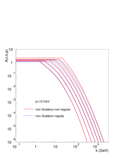
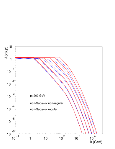
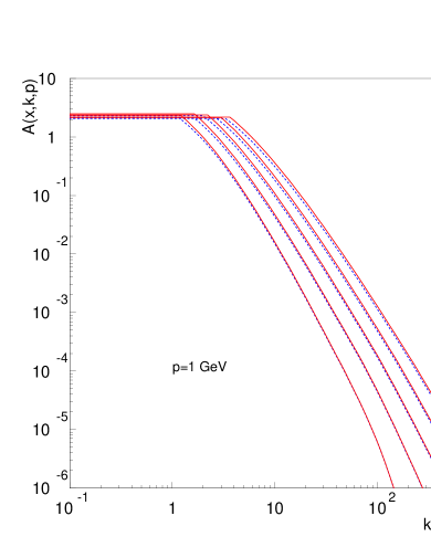
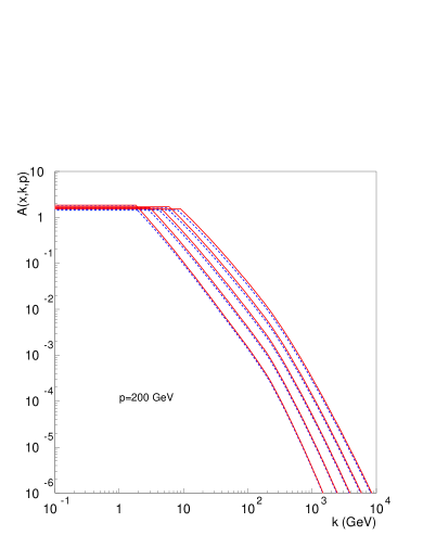
In figure 10 we show the solution to the CCFM with the saturation boundary implemented in the form of freezing as in (4.32). Here, the coupling is fixed . We compare solutions obtained using (2.6) and (2.7) respectively. We see that once the saturation effects are included, the differences between the solutions using the different form-factors are not that large, as the sensitive infrared region is regularized by the saturation boundary. The dependence on can be examined by comparing the left and right plot in figure 10. We observe that, similarly to the linear case, the distributions change slopes when become comparable to the external scale . For , the gluon distribution is effectively cut off by the scale .
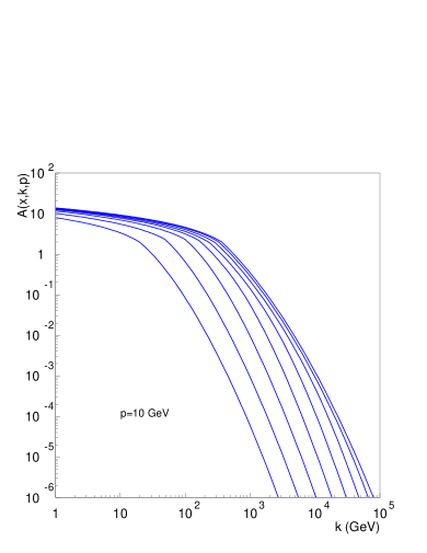
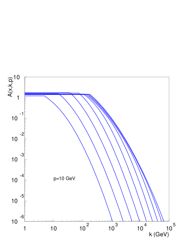
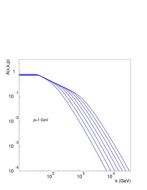
In order to analyze the asymptotic behavior of the solutions we extend the rapidity range up to . This is shown in figure 11, where we use the non-Sudakov form-factor from equation (2.6). We observe the interesting effect that the front of the solution no longer travels to higher momenta with uniform ’speed’ governed by the saturation scale, but that it rather stalls at high rapidities. The origin of this behavior is rooted in the presence of the additional scale . As the rapidity grows, the solution diffuses to the higher values of the transverse momenta . At the same time the saturated region grows also with energy. The unsaturated region is eventually pushed to the region where , which is then cut off by the angular ordering condition. Therefore the phase space for new emissions is squeezed, due to the presence of two scales and . We have done the analysis with two different boundaries (4.31) (logarithmic growth at low momenta) and (4.32) (freezing) and it is clear that the front stops to diffuse to higher momenta in both cases. The stalling of the front therefore is a robust feature of CCFM with saturation as it does not depend on the way the boundary is implemented. We note that the complete stalling of the front (in the case presented in figure 11) occurs for momenta , which is order of magnitude larger than the . In consequence, the saturation scale starts to behave differently with rapidity in this regime. In particular the value of will no longer scale linearly with rapidity but slower than that, and eventually the saturation scale will ’saturate’ itself at large . The complete analysis of the behavior of the saturation scale is presented in the later section.
5.2 Running coupling results
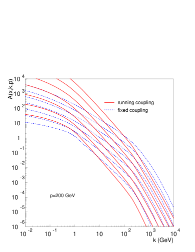
Let us now turn the case of a running coupling. In figure 12 we show the different results obtained using the two different form factors, (2.6) and (2.7). Here, the boundary condition (4.32) is used, and is used as scale in . As in the fixed coupling case we see that the differences are much smaller than in the linear evolution, and almost identical results are obtained. In particular we have checked that the small difference between the results stays the same up to very large values of (far beyond phenomenologically relevant values). We find that, apart from the region of smallest in the figures, the difference is a normalization factor independent of and . Consequently the different form factors lead to almost identical saturation scales which we shall look more closely at in the next section.
Since in the running coupling case the evolution is generally slowed down, one needs to go to higher values of to see the stalling of . For larger in fact, the values required for the stalling are so extremely large that we have not reached them in our numerical solution. Starting from smaller values, however, we clearly see how the evolution is eventually slowed down to a point where starts to stall in a region between and (i.e. around ), and one can also see how this region then grows with . Increasing we see that one needs ever higher to see this behavior (as in the fixed coupling case).
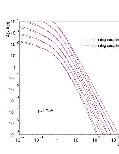
In figure 13 we show the extension of the solution shown in the left plot of figure 12 (that is when GeV) to asymptotic values of between 46 and 70 units. In this case only the solution using (2.7) is presented, the solution using (2.6) looks essentially the same. Compared to the fixed coupling case, the region where stalls is much smaller, and it also grows slower. Therefore the saturation of the saturation scale will set in much later (to be shown in the next section). To be able to exactly determine at what the stalling of starts to become visible, we would need to know the full non-linear formulation of CCFM. The application of different boundary conditions seem to, however, indicate that this behavior sets in rather late, as manifest in figure 13. Moreover there are additional effects not taken into account here (such as energy conservation) which will further slow down the evolution.
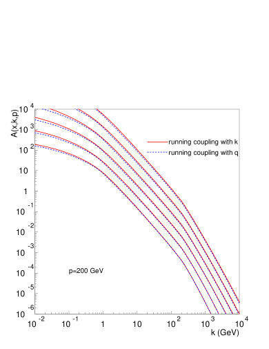
Let us now turn to the implementation of different scales in . In the linear case we observed the fact that generally the choice of gives a slower evolution compared to the default choice . In figure 14 we show the comparison between the results obtained from the two different scales. For the larger values the differences between the two choices of scales are very small. For smaller values of the differences are more pronounced, the solution with scale being consistently smaller than with the choice of scale . As explained earlier in section 2.3.3, this effect is due to the stronger suppression from when is selected as scale.
This, however, brings us to another point. Namely the fact that one should actually not allow any contribution to the non-Sudakov form factor from the region which lies outside the region set by the maximal angle , or equivalently by . To understand this, remember the derivation of shown in figures 3 and 4. The regions in that case were bounded by the maximal angle . When , it can be that region partly, or completely, lies outside the region bounded by . In that case also parts of region will be located outside the allowed region (however, cannot lie completely outside the allowed region). In reality, however, one should not include any contribution from those parts of and (actually since only figure 3 and the corresponding regions and are relevant). Thus one should in equation (2.3) actually only include the part of region which is bounded by . By not doing this one is generally overestimating the suppression from when . The non-Sudakov form factor will then be modified, and it will depend not only on , and , but also on and the previous values of in the chain. Unfortunately this also implies that it is no longer possible to write an integral equation as in (2.1) or (2.2) because one needs to keep track of all values in each during the evolution (this is because then depends not only the vertex but also on earlier vertices). One can only write down the gluon distribution in an unfolded form, explicitly summing it over all possible chains.
Thus when using the scale instead of we do find some differences in the evolution. On the other hand, for reasonable values of these differences are rather small, and for values around 10 GeV and higher they are negligible. We will also see in the next section that the respective saturation momenta are quite similar, despite the noted differences. We have also noted that when one should actually modify to be consistent. However, the implementation of this modification is probably in practice only feasible in a MC simulation where one can keep track of the history of the entire gluon chain.
5.3 The saturation scale
Fixed coupling results
From the solutions to the gluon distribution one can extract the saturation scale . We have already commented on the definition of in section 4. The exact value of the constant defining only affects its normalization which we cannot control anyhow, the and dependences are independent of the value of this constant (of course the constant should not be varied over many orders of magnitude).


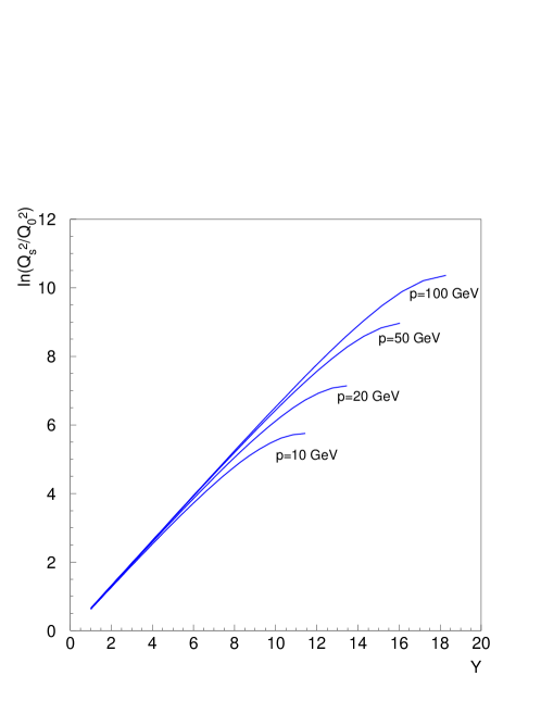
In figure 15 we show the results for the two different boundary conditions (4.31) and (4.32) when the coupling is fixed and the non-Sudakov in (2.7) is used. In both cases we find a behavior consistent with the expectation in (3.25) which holds as long as . As grows above , as is most visible in the case when GeV in figure 15, we see that the growth of on rapidity becomes non-linear. The range shown in the figure is similar to what is accessed at the LHC. The absolute values of should not be considered as realistic estimates of what would be at the LHC (a fixed coupling calculation is not so relevant phenomenologically anyway). The two different boundary conditions give rise to slightly different dependences for for each given , but the differences are rather small.

The rather dramatic change in the dependence of is visible in figure 16 where we extend the results from figure 15 to much larger (far beyond experimentally accessible values). As we see, the general shape of does not depend on the precise boundary being used. We see that once , the dependence of on becomes non-linear, and eventually it saturates to some value depending on . Of course we cannot say exactly whether there exist a given constant such that as or whether keeps growing, albeit extremely slowly. Nevertheless, it is clear that, the growth of on rapidity saturates and that the dependence of on is highly non-linear. Interestingly, we observe that there exists a certain scaling in the sense that once has saturated, the ratio between the values for two given values of is independent of . In other words, we find that the ratio is a constant independent of , once . The value of this constant depends on the precise boundary condition used, for example for the boundary in (4.31) we find when is very large, while for the boundary in (4.32) we instead get .


Next we investigate the results obtained using the non-Sudakov in
(2.6). In this case since the normalization of is larger, the
normalization of will also be larger. We only show the results using the
boundary condition (4.31), the results for (4.32) are similar.
The plots for are shown in figure 17 and we find exactly the same
type of behavior as above. This is further seen from the right figure where the comparison
to the above results are shown. As can be seen, the energy dependence of is the same
regardless of the non-Sudakov chosen, and we find the difference in normalization to
be a factor roughly 1.35, regardless of the value of .
Running coupling results
It is well known that the growth of is slowed down by the running of the coupling. Physically it is of course consequence of the fact that the evolution leads to the diffusion towards higher transverse momenta where the coupling is much smaller. In BFKL, the linear dependence at fixed coupling is for a running coupling replaced by where for , . In CCFM we again expect to find a BFKL-like behavior as long as . As a consequence of the much slower growth, one needs thus in the running coupling case much higher values in order to reach the point where . This implies that the stalling of the growth, and the consequent saturation of is delayed to higher energies.
We start by again comparing the effects of different boundary conditions. In addition to the two boundary conditions presented above, we also try an additional boundary where we simply fix to be a given constant behind the saturation front. In particular we choose
| (5.33) |
We will with this choice further demonstrate the robustness of the method.


In figure 18 we compare different boundary conditions for both of the non-Sudakov form factors. We see that the differences are minor and that they can be removed by and independent scale factors. For both cases we find a difference in scaling of around a factor 1.20. We also see that as in BFKL grows much slower and also that, as a consequence, the dependence on is weaker. As in the fixed coupling case, as long as we find a BFKL-like behavior, thus in the phenomenologically relevant interval shown in the figure we find that for GeV, grows proportional to . As becomes comparable to , however, this dependence is altered and becomes more complicated. Continuing to larger , one again finds that eventually saturates. From figure 19 we also see that the difference between the results for two non-Sudakov form factors are rather minor, and turns out to be a pure scaling, around a factor 1.10, independent of and . These results show that seemingly very different linear evolutions obtained from the different non-Sudakov form factors give almost identical results once saturation is properly implemented. In this way any potential ambiguity of the formalism is removed. We note also that it was demonstrated in [15] that the explicit inclusion of the kinematical constraint again only leads to a different normalization, once saturation is implemented.


In order to demonstrate the saturation of we extend in figure 20 the running coupling results to asymptotic values of . Once again we see the complete saturation of for smaller , but in this case one needs much larger values to reach the stalling region. Furthermore we see that the scaling behavior noted above in the fixed coupling case, namely that saturates to a number independent than , is no longer true when the coupling is running. Additionally, as in the previous figures, we see that the dependence on is much weaker than in the fixed coupling case.
Next, we extract in the case when is used as scale for the running coupling. As we have seen from the results for the gluon distribution, the evolution for smaller is generally slowed down in this case, and consequently we find a slower growing saturation scale. The results are shown in figure 21. Since the evolution is generally slower, the dependence for smaller is also weaker. For phenomenologically interesting values, however, the differences are not that large. In all the results presented here for one should keep in mind that the estimates are highly optimistic, in the sense that is rather large already at low . From phenomenological analysis performed at HERA, we do not expect to find such a large normalization of at the LHC. We discuss the phenomenological relevance of our method in the next section.

Finally let us mention that, though not shown, we have also checked that the conclusions are not altered when a different set of the boundary parameters are used. In addition to the default choice , we have also used , and , . The different choices lead to different normalizations of but do not alter the or dependence. The method is therefore rather general and robust.
6 Summary and outlook
In this paper we have analyzed the nonlinear effects in the CCFM equation using a boundary method. We have found that, the resulting gluon distribution exhibits similar properties as in previous BFKL/BK studies only in the region of transverse momenta lower than the scale in CCFM. As the rapidity grows and the momenta diffuse to the higher values, the dependence on the rapidity and becomes highly complicated, and completely novel effects are observed. As a result the diffusion of the transverse momenta to higher values is significantly suppressed due to angular ordering when the typical scales exceed . For ultrahigh rapidities this results in the stalling of the propagation front of the solution.
From the gluon distribution we have extracted the saturation scale in CCFM. We have found that due to the presence of the additional scale in CCFM, the saturation scale becomes also dependent on this scale. Also, the high rapidity behavior of the saturation scale is significantly modified in CCFM. For ultrahigh rapidities the saturation scale stops to grow completely, and this is related to the above-mentioned stalling of the gluon distribution. The smaller the value of , the lower are the rapidities for which deviations from the BK-type behavior of the saturation scale are observed. Analytical calculations confirm the numerical analysis on the behavior of the saturation scale.
We have investigated the cases both in fixed and running coupling scenarios, and found that in the running coupling case the novel features are present, yet for the higher values of rapidities. We have also investigated the dependence of the gluon distribution on the choice of the non-Sudakov form-factors. In the case when the boundary is present there is very little sensitivity of the solutions on the different form factors, due to the fact that the nonlinear effects basically regularize the infrared region where the differences are the largest. On the other hand, in the linear case we have found that the different forms of the form factors lead to large discrepancies of the solutions.
Let us now comment on the possible phenomenological relevance and importance of the method and results presented here. The results obtained here indicate that the saturation of occurs at extremely large values of rapidity. In the phenomenologically relevant case of the running coupling, the rapidities needed to observe this phenomenon are about . Such extremely large values are not accessible at present particle colliders. One should also take into account the fact that here we only included the term of the splitting function. The other, nonsingular at terms are important too and they are known to reduce the speed of the rapidity evolution. One also needs to properly take into account the effects of the energy momentum conservation which will further reduce the growth. Taking these effects into consideration we can conclude that it will be very difficult to observe the novel effect of saturation of in the near future. One the other hand one needs to note that the exact values of the rapidities at which stalling occurs could depend on the details of the initial condition. What could be however relevant phenomenologically is the dependence of the saturation scale on the additional scale in the regime where is of order . For example in DIS, in the usual saturation-based approaches one treats and as completely independent scales. The results of our analysis indicate that saturation scale should be correlated with when both scales are of the same order.
The interesting question is, however, whether or not it is urgent to introduce saturation effects for studies at LHC involving unintegrated parton densities. This question is relevant and important, as saturation affects the shape of the unintegrated distributions, even at higher . Usually the distributions are extracted using linear evolution equations and they will be used in almost every physics analysis at the LHC. A recent study [34] has reported deviations from small- resummed DGLAP evolution in the HERA data that might be related to saturation effects. Therefore we think that there is a need to analyze the possible saturation effects in the evolution and their impact onto the LHC observables with substantial precision.
To study in more detail the relevance of saturation, one would first have to include additional corrections to the hard emissions. Obviously the soft emissions associated with the pole are important to include as well as the other non-singular terms in of the splitting function. We intend to return to this issue in a future publication. The soft emissions are included in the CASCADE event generator, and as already outlined in [14, 15], the boundary method can be implemented in an event generator much in the same way. A first attempt of applying a boundary method in CASCADE was reported in [35]. In this case, however, was assumed a priori to be of the standard form [19], and it was then used as a cut-off in . As we have seen here, in CCFM depends on rapidity and in much more complicated way. Moreover, the power of the boundary method is that it gives a consistent with the evolution.
A problem we see with the application of the boundary method in CASCADE is that the results coming from it show almost no growth at all of from the small- evolution. The relatively steep growth in needed to fit data at HERA is rather provided by the dependence of the off-shell hard matrix element and the initial condition. Obviously, if there is very little growth coming from the perturbative gluon cascade, then saturation will not be relevant.
A similar effect is observed in the resummed BFKL/DGLAP approaches [30, 29, 36, 37, 38, 39, 40, 41, 42]. It was consistently found that the resummed gluon-gluon splitting function does indeed have the singularity at small , but the subleading corrections cause the resummed splitting function to be very close numerically to NLO DGLAP in the region . Therefore in the kinematic regime covered by HERA the evolution of the gluon distribution is controlled by the DGLAP equations. On the other hand it was found in earlier analysis [32] that when evaluating structure function from the factorization approach together with unintegrated gluon distribution, large enhancement in the low region is provided by the off-shell matrix element, similarly to what was observed in CASCADE.
A related problem was also reported in [43] where some phenomenological applications of CCFM were presented. In that case, again only the hard emissions were included, but to simulate possible non-leading effects, the non-Sudakov (2.7) was modified by simply changing the integration intervals, resulting in a larger suppression coming from the form factor (the exact motivation for this change was given by checking that the resulting high energy saddle point more or less agree with the one extracted from NLL BFKL studies). The result was that the small- growth turned out be much delayed again, and as discussed in that paper this delay might be behind the fact that CCFM predictions on forward jets seem to underestimate the growth of the jet cross section with decreasing (for recent studies of forward jets within CASCADE see [44, 45]).
On the other hand, a reason why one has to introduce a strong suppression from additional effects, which then delay the small- growth, is because it is otherwise not possible to fit from the linear evolution. This is not so surprising since the linear evolution at small momenta gives a very strong growth which we know must be tamed by non-linear effects. Even if one only performs a fit to for moderate values of , because one is integrating to smaller , saturation effects are not completely negligible. One can therefore imagine that a procedure like that in [43], where the non-leading effects were introduced by hand, easily overestimates the suppression coming from them when saturation effects are not properly included. On the other hand the non-leading pieces are more properly included in CASCADE which has the same problems as in [43]. An event generator is, however, rather complex, including many different components, and it is not always very transparent how big the role of the first principle physics in it is. Therefore we believe it will be very valuable to include the soft emissions in a simple numerical simulation as done here, so that one can more closely study the combined effects of the different physics components in a simpler environment. This may shed light on the possible relevance of saturation for hard physics at the LHC (obviously for the possible description of the Underlying Event (UE) saturation effects such as multiple scatterings etc are very important. For a possible description of the very complex UE at the LHC one will need an entirely different approach to the problem, for some recent articles on this issue see [46, 47]).
Acknowledgments
This work is partially supported by U.S. D.O.E. grant number DE-FG02-90-ER-40577, U.S. D.O.E. OJI grant number DE-SC0002145 and MNiSW grant number N202 249235. A.M.S. is also supported by the Sloan Foundation.
References
-
[1]
L.N. Lipatov, Sov. J. Nucl. Phys. 23 (1976) 338;
E.A. Kuraev, L.N. Lipatov and V.S. Fadin, Zh. Eksp. Teor. Fiz 72, 3 (1977) (Sov. Phys. JETP 45 (1977) 199);
Ya.Ya. Balitsky and L.N. Lipatov, Sov. J. Nucl. Phys. 28 (1978) 822. - [2] M. Ciafaloni, Nucl. Phys. B296 (1988) 49.
- [3] S. Catani, F. Fiorani and G. Marchesini , Nucl. Phys. B336 (1990) 18.
- [4] S. Catani, F. Fiorani, and G. Marchesini, Phys. Lett. B234 (1990) 339.
- [5] G. Marchesini, Coherence and small x cascade, Nucl. Phys. Proc. Suppl. 39BC (1995) 18–21.
- [6] G. Marchesini, Structure function for large and small x, . Prepared for INFN Eloisatron Project, 17th Workshop: QCD at 200 TeV, Erice, Italy, 11-17 Jun 1991.
- [7] L. D. McLerran and R. Venugopalan, Computing quark and gluon distribution functions for very large nuclei, Phys. Rev. D49 (1994) 2233–2241, [hep-ph/9309289].
- [8] L. D. McLerran and R. Venugopalan, Gluon distribution functions for very large nuclei at small transverse momentum, Phys. Rev. D49 (1994) 3352–3355, [hep-ph/9311205].
-
[9]
E. Iancu, Color Glass Condensate and its relation to HERA physics,
arXiv:0901.0986 [hep-ph];
A.H. Mueller, Parton Saturation–An Overview, hep-ph/0111244;
E. Iancu, A. Leonidov and L. McLerran, The Colour Glass Condensate: An Introduction, hep-ph/0202270. Published in QCD Perspectives on Hot and Dense Matter, Eds. J.-P. Blaizot and E. Iancu, NATO Science Series, Kluwer, 2002;
E. Iancu and R. Venugopalan, The Color Glass Condensate and High Energy Scattering in QCD, hep-ph/0303204. Published in Quark-Gluon Plasma 3, Eds. R.C. Hwa and X.-N. Wang, World Scientific, 2003;
H. Weigert, Evolution at small : The Color Glass Condensate, Prog. Part. Nucl. Phys. 55 (2005) 461 [hep-ph/0501087]. - [10] I. Balitsky, Operator expansion for high-energy scattering, Nucl. Phys. B463 (1996) 99–160, [hep-ph/9509348].
- [11] Y. V. Kovchegov, Small-x F2 structure function of a nucleus including multiple pomeron exchanges, Phys. Rev. D60 (1999) 034008, [hep-ph/9901281].
- [12] J. Jalilian-Marian, A. Kovner, A. Leonidov and H. Weigert, Nucl. Phys. B504 (1997) 415; Phys. Rev. D59 (1999) 014014; J. Jalilian-Marian, A. Kovner and H. Weigert, Phys. Rev. D59 (1999) 014015; A. Kovner, J. G. Milhano and H. Weigert, Phys. Rev. D62 (2000) 114005.
- [13] E. Iancu, A. Leonidov and L. McLerran, Nucl. Phys. A692 (2001) 583; Phys. Lett. B510 (2001) 133; E. Ferreiro, E. Iancu, A. Leonidov and L. McLerran, Nucl. Phys. A703 (2002) 489; E. Iancu and L. McLerran, Phys. Lett. B510 (2001) 145.
- [14] E. Avsar and E. Iancu, BFKL and CCFM evolutions with saturation boundary, Phys. Lett. B673 (2009) 24–29, [arXiv:0901.2873].
- [15] E. Avsar and E. Iancu, CCFM Evolution with Unitarity Corrections, Nucl. Phys. A829 (2009) 31–75, [arXiv:0906.2683].
- [16] A. H. Mueller and D. N. Triantafyllopoulos, The energy dependence of the saturation momentum, Nucl. Phys. B640 (2002) 331–350, [hep-ph/0205167].
- [17] E. Iancu, K. Itakura, and L. McLerran, Geometric scaling above the saturation scale, Nucl. Phys. A708 (2002) 327–352, [hep-ph/0203137].
- [18] B. Andersson, G. Gustafson, and J. Samuelsson, The linked dipole chain model for dis, Nucl. Phys. B467 (1996) 443–478.
- [19] A. M. Stasto, K. Golec-Biernat, and J. Kwiecinski, Geometric scaling for the total gamma* p cross-section in the low x region, Phys. Rev. Lett. 86 (2001) 596–599, [hep-ph/0007192].
- [20] H. Jung and G. P. Salam, Hadronic final state predictions from CCFM: The hadron- level Monte Carlo generator CASCADE, Eur. Phys. J. C19 (2001) 351–360, [hep-ph/0012143].
- [21] J. Kwiecinski, A. D. Martin, and P. J. Sutton, The gluon distribution at small x obtained from a unified evolution equation, Phys. Rev. D52 (1995) 1445–1458, [hep-ph/9503266].
- [22] G. Marchesini and B. R. Webber, Simulation of QCD initial state radiation at small x, Nucl. Phys. B349 (1991) 617–634.
- [23] V. S. Fadin and L. N. Lipatov, Next-to-leading Corrections to the BFKL Equation From the Gluon and Quark Production, Nucl. Phys. B477 (1996) 767–808, [hep-ph/9602287].
- [24] V. S. Fadin, M. I. Kotsky, and L. N. Lipatov, One-loop correction to the BFKL kernel from two gluon production, Phys. Lett. B415 (1997) 97–103.
- [25] V. S. Fadin and L. N. Lipatov, BFKL pomeron in the next-to-leading approximation, Phys. Lett. B429 (1998) 127–134, [hep-ph/9802290].
- [26] G. Camici and M. Ciafaloni, Non-abelian q anti-q contributions to small-x anomalous dimensions, Phys. Lett. B386 (1996) 341–349, [hep-ph/9606427].
- [27] G. Camici and M. Ciafaloni, Irreducible part of the next-to-leading BFKL kernel, Phys. Lett. B412 (1997) 396–406, [hep-ph/9707390].
- [28] M. Ciafaloni and G. Camici, Energy scale(s) and next-to-leading BFKL equation, Phys. Lett. B430 (1998) 349–354, [hep-ph/9803389].
- [29] M. Ciafaloni, D. Colferai, G. P. Salam, and A. M. Stasto, Renormalisation group improved small-x Green’s function, Phys. Rev. D68 (2003) 114003, [hep-ph/0307188].
- [30] M. Ciafaloni, D. Colferai, D. Colferai, G. P. Salam, and A. M. Stasto, Extending QCD perturbation theory to higher energies, Phys. Lett. B576 (2003) 143–151, [hep-ph/0305254].
- [31] G. Bottazzi, G. Marchesini, G. P. Salam, and M. Scorletti, Structure function and angular ordering at small x, Nucl. Phys. B505 (1997) 366–386, [hep-ph/9702418].
- [32] J. Kwiecinski, A. D. Martin, and A. M. Stasto, A unified BFKL and GLAP description of F2 data, Phys. Rev. D56 (1997) 3991–4006, [hep-ph/9703445].
- [33] G. P. Salam, A resummation of large sub-leading corrections at small x, JHEP 07 (1998) 019, [hep-ph/9806482].
- [34] F. Caola, S. Forte, and J. Rojo, Deviations from NLO QCD evolution in inclusive HERA data, arXiv:0910.3143.
- [35] K. Kutak and H. Jung, Saturation effects in final states due to CCFM with absorptive boundary, Acta Phys. Polon. B40 (2009) 2063–2070, [arXiv:0812.4082].
- [36] M. Ciafaloni, D. Colferai, G. P. Salam, and A. M. Stasto, The gluon splitting function at moderately small x, Phys. Lett. B587 (2004) 87–94, [hep-ph/0311325].
- [37] M. Ciafaloni, D. Colferai, G. P. Salam, and A. M. Stasto, A matrix formulation for small-x singlet evolution, JHEP 08 (2007) 046, [arXiv:0707.1453].
- [38] G. Altarelli, R. D. Ball, and S. Forte, Resummation of singlet parton evolution at small x, Nucl. Phys. B575 (2000) 313–329, [hep-ph/9911273].
- [39] G. Altarelli, R. D. Ball, and S. Forte, Factorization and resummation of small x scaling violations with running coupling, Nucl. Phys. B621 (2002) 359–387, [hep-ph/0109178].
- [40] G. Altarelli, R. D. Ball, and S. Forte, An anomalous dimension for small x evolution, Nucl. Phys. B674 (2003) 459–483, [hep-ph/0306156].
- [41] G. Altarelli, R. D. Ball, and S. Forte, Perturbatively stable resummed small x evolution kernels, Nucl. Phys. B742 (2006) 1–40, [hep-ph/0512237].
- [42] G. Altarelli, R. D. Ball, and S. Forte, Small x Resummation with Quarks: Deep-Inelastic Scattering, Nucl. Phys. B799 (2008) 199–240, [arXiv:0802.0032].
- [43] G. Bottazzi, G. Marchesini, G. P. Salam, and M. Scorletti, Small-x one-particle-inclusive quantities in the CCFM approach, JHEP 12 (1998) 011, [hep-ph/9810546].
- [44] M. Deak, F. Hautmann, H. Jung, and K. Kutak, Jets in the forward region at the LHC, arXiv:0908.1870.
- [45] M. Deak, F. Hautmann, H. Jung, and K. Kutak, Forward Jet Production at the Large Hadron Collider, JHEP 09 (2009) 121, [arXiv:0908.0538].
- [46] G. Gustafson, Multiple Interactions, Saturation, and Final States in pp Collisions and DIS, Acta Phys. Polon. B40 (2009) 1981–1996, [arXiv:0905.2492].
- [47] C. Flensburg and G. Gustafson, Fluctuations, Saturation, and Diffractive Excitation in High Energy Collisions, arXiv:1004.5502.