Transport implications of Fermi arcs in the pseudogap phase of the cuprates

Abstract

We derive the fermionic contribution to the longitudinal and Hall conductivities within a Kubo formalism, using a phenomenological Greens function which has been previously developed to describe photoemission data in the pseudogap phase of the cuprates. We find that the in-plane electrical and thermal conductivities are metallic-like, showing a universal limit behavior characteristic of a d-wave spectrum as the scattering rate goes to zero. In contrast, the c-axis resistivity and the Hall number are insulating-like, being divergent in the same limit. The relation of these results to transport data in the pseudogap phase is discussed.

Photoemission data for underdoped cuprates reveal that the Fermi surface in the pseudogap phase breaks up into disconnected Fermi segments, known as Fermi arcs.Nat98 The length of these arcs scales linearly with $T/T^{*}(x)$, where $T^{*}(x)$ is the doping dependent pseudogap temperature.Amit This behavior can be reproduced if one assumes a temperature independent d-wave gap with a scattering rate proportional to $T$.Tallon ; Norm07

Obviously, such temperature dependent arcs should have profound implications for the nature of the transport in the pseudogap phase.Ando To investigate this, we take a Greens function based on a phenomenological self-energy that generates these arcs,PRB98 ; Norm07 and then construct the Kubo bubble. We use this to calculate both the in-plane and c-axis longitudinal conductivities, as well as the Hall conductivity. We then connect our results to transport data for the cuprates.

The in-plane conductivity at T=0 is given by the Kubo formula Mahan

$$\sigma_{xx}=\frac{2e^{2}\hbar}{\pi}\int\frac{d^{3}k}{(2\pi)^{3}}v_{x}^{2}(k)[\mathrm{Im}G(k,0)]^{2}$$ (1)

where $v_{x}$ is the $x$ component of the Fermi velocity, $\mathrm{Im}G(k,0)\equiv\mathrm{Im}G^{R}(k,\omega=0)$ with $G^{R}$ the retarded Greens function, and the factor of 2 comes from summing over spin. Transforming the $k$ integral to one over $\epsilon$ and $\phi$, and ignoring the $\phi$ dependence of $v$ and any c-axis dispersion, we have the planar conductivity

$$\sigma=\frac{e^{2}\hbar Nv^{2}}{\pi d}\int d\epsilon\frac{d\phi}{2\pi}[\mathrm{Im}G(\epsilon,\phi,0)]^{2}$$ (2)

where $N$ is the (two dimensional) normal state density of states (per spin), $v$ the Fermi velocity, and $d$ the c-axis thickness divided by the number of conducting planes.

We now consider a BCS model for the Greens function. In the so-called ‘single lifetime’ version,PRB98 ; Tallon ; Norm07

$$-\mathrm{Im}G(\epsilon,\phi,0)=\frac{\Gamma}{\epsilon^{2}+\Gamma^{2}+\Delta^{2}(\phi)}$$ (3)

where $\Delta$ is the pairing gap and $\Gamma$ the inverse lifetime.foot1 This form for $G$ gives a good description of photoemission data in the pseudogap phase. In particular, if $\Gamma$ scales as $T$, then the $T$ dependence of the arc length is reproduced, as well as the variation of the spectral gap around the Fermi surface.

Substituting this form of $G$ into the expression for $\sigma$, the $\epsilon$ integral is convergent, and setting its limits to infinity yields

$$\sigma=\frac{e^{2}\hbar Nv^{2}\Gamma^{2}}{\pi d}\int_{0}^{\pi/2}\frac{dx}{(\Gamma^{2}+\Delta_{0}^{2}\cos^{2}x)^{3/2}}$$ (4)

where in the d-wave case, $\Delta(\phi)=\Delta_{0}\cos x$ with $x=2\phi$. Performing the $x$ integration

$$\sigma=\frac{e^{2}\hbar Nv^{2}\lambda}{\pi d\Delta_{0}}E(\lambda)$$ (5)

where $\lambda=\Delta_{0}/\sqrt{\Gamma^{2}+\Delta_{0}^{2}}$ and $E$ is the complete elliptic integral of the second kind.

This can be easily generalized Ioffe to the case of the c-axis conductivity by replacing $v^{2}/2$ by $t^{2}_{\perp}(\phi)d^{2}/\hbar^{2}$, where $t_{\perp}$ is the interlayer tunneling energy whose angle dependence goes as $\cos^{2}(2\phi)$.PWA ; Ole This has a profound effect on the conductivity,LeeRMP

$$\sigma_{c}=\frac{2e^{2}dNt_{\perp}^{2}\Gamma^{2}}{\pi\hbar}\int_{0}^{\pi/2}\frac{dx\cos^{4}(x)}{(\Gamma^{2}+\Delta_{0}^{2}\cos^{2}x)^{3/2}}$$ (6)

Evaluating, one finds

$$\sigma_{c}=\frac{2e^{2}dNt_{\perp}^{2}\Gamma^{2}}{\pi\hbar\Delta_{0}^{3}\lambda}[(2-\lambda^{2})E(\lambda)-2(1-\lambda^{2})K(\lambda)]$$ (7)

where $K$ is the complete elliptic integral of the first kind.

In Fig. 1, the inverse of $\sigma$ ($\rho$) and $\sigma_{c}$ ($\rho_{c}$) are plotted as a function of $\Gamma$. For zero $\Delta_{0}$, they are proportional to $\Gamma$ as expected. For non-zero $\Delta_{0}$, it is seen that $\rho$ saturates to a finite value in the limit that $\Gamma$ goes to zero. This is the universal limit discussed by Patrick Lee.Lee The resistance has a weak minimum when $\Gamma/\Delta_{0}\sim 0.46$, before increasing like $\Gamma$ as in the normal state. The c-axis conductivity behaves quite differently because of the $\cos^{4}(2\phi)$ factor, which is peaked at $\phi=0$ where the d-wave gap is maximal (thus killing off the universal behavior associated with the nodes). As a consequence, $\rho_{c}$ diverges as $1/\Gamma^{2}$ (this behavior coming from the prefactor in Eq. 6). As $\Gamma$ increases, a strong minimum is seen in $\rho_{c}$ at $\Gamma/\Delta_{0}\sim 1.26$, before increasing like $\Gamma$.

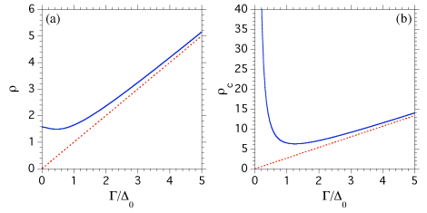
Figure 1: (Color online) (a) planar and (b) c-axis resistivity versus $\Gamma$. The units for $\rho$ are $2m^{*}/(e^{2}\hbar n)$ and for $\rho_{c}$ are $\hbar^{2}v^{2}m^{*}/(d^{2}e^{2}\hbar nt_{\perp}^{2})$, where $n/m^{*}=Nv^{2}/d$ with $n$ the electron density and $m^{*}$ the effective mass. The dashed lines are for $\Delta_{0}=0$.

Although the above results are for $T$=0, we have done numerical studies which included the thermal factors in the Kubo bubble. Only minor differences were seen, and thus to a good approximation, the above $T$=0 formulas are sufficient. Therefore, if $\Delta_{0}$ is constant, and $\Gamma$ scales as $T$, as commonly assumed to describe the photoemission data, then the x-axis of the above figures can be read as temperature.

We now turn to the Hall conductivity (current in the plane, field along the c-axis) which is easily derived by insertion of a magnetic field vertex into the Kubo bubble foot2

$$\sigma_{H}=-\frac{2e^{2}\hbar^{2}Nv^{2}\omega_{c}}{3\pi d}\int d\epsilon\frac{d\phi}{2\pi}[\mathrm{Im}G(\epsilon,\phi,0)]^{3}$$ (8)

where $\omega_{c}$ is the cyclotron frequency ($eH/m^{*}c$). Substituting $G$ from Eq. 3 and performing the integral over $\epsilon$

$$\sigma_{H}=\frac{e^{2}\hbar^{2}Nv^{2}\Gamma^{3}\omega_{c}}{2\pi d}\int_{0}^{\pi/2}\frac{dx}{(\Gamma^{2}+\Delta_{0}^{2}\cos^{2}x)^{5/2}}$$ (9)

Evaluating, one finds

$$\sigma_{H}=\frac{e^{2}\hbar^{2}Nv^{2}\omega_{c}\lambda}{6\pi d\Gamma\Delta_{0}}[2(2-\lambda^{2})E(\lambda)-(1-\lambda^{2})K(\lambda)]$$ (10)

Note that the Hall resistivity ($\rho_{H}$) is $\sigma_{H}/\sigma^{2}$, and the Hall coefficient ($R_{H}$) is $\rho_{H}/H$.

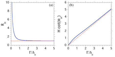
Figure 2: (Color online) (a) Hall coefficient and (b) cotangent of the Hall angle versus $\Gamma$. The units for $R_{H}$ are $1/(nec)$ and $H\cot(\Theta_{H})$ are $2cm^{*}/(e\hbar)$. The dashed lines are for $\Delta_{0}=0$.

In Fig. 2a, we plot the Hall number as a function of $\Gamma$, where it is seen to diverge as $1/\Gamma$ at small $\Gamma$. This behavior is due to the nodal contribution, thus generalizing the results of Ref. Lee, to the Hall conductivity. In Fig. 2b, we plot the cotangent of the Hall angle, $H\cot(\Theta_{H})=\rho/R_{H}$, which vanishes as $\Gamma$ goes to zero, but increases as $\Gamma$ for large $\Gamma$.

These results are easily generalized to their thermal counterparts.Paul The in-plane thermal conductivity is

$$\kappa_{xx}=\frac{2\pi\hbar k_{B}^{2}T}{3}\int\frac{d^{3}k}{(2\pi)^{3}}v_{x}^{2}(k)[\mathrm{Im}G(k,0)]^{2}$$ (11)

and thus we recover Durst the Wiedemann-Franz law $\kappa=\frac{\pi^{2}k_{B}^{2}T\sigma}{3e^{2}}$ (therefore, $\kappa$ exhibits universal behavior as well). For the thermopower, $S$, and the Nernst, one must consider particle-hole asymmetry effects. In our simple model where $\Gamma$ is taken as a momentum and frequency independent constant, the only source for this is the density of states, $N$. As a consequence, we find that $S/T$ is a constant ($\frac{\pi^{2}k_{B}^{2}}{3e}\frac{d\ln N}{d\epsilon}$), and that the Nernst effect vanishes due to the Sondheimer cancellation (i.e., $\frac{\partial\tan(\Theta_{H})}{\partial\epsilon}=0$). These results will obviously change if a more sophisticated model is used for the self-energy.Paul

We now discuss implications of our results. The first point we wish to make is almost trivial. That is, transport data for various dopings scale as a function of $T/T^{*}(x)$.Wuyts ; Luo Since $\Delta_{0}$ scales with $T^{*}(x)$ JC99 and $\Gamma$ with $T$,MFL then our transport results also scale as $T/T^{*}(x)$. Within our model, the scaling factor is such that $\Gamma=\sqrt{3}\Delta_{0}T/T^{*}$, noting that $\Gamma/\Delta_{0}>\sqrt{3}$ is the condition for gaplessness of $\mathrm{Im}G(\epsilon=0,\phi=0,\omega)$.Norm07 Since $\Delta_{0}/T^{*}\sim 2$, this reduces to $\Gamma\sim 2\sqrt{3}T$.

Now, as the arc length scales with $\Gamma$, one might have naively expected that the planar resistivity would diverge as $\Gamma$ goes to zero. This does not occur for the same reasons discussed by Lee.Lee That is, for a d-wave spectral gap, the residual conductivity is independent of the scattering rate. This result, though, does not hold for the c-axis resistivity, which indeed diverges. Experimentally, the in-plane resistivity is indeed metallic-like in the pseudogap phase, whereas the c-axis resistivity is divergent.Timusk So, this basic dichotomy of the cuprates is trivially explained by our model. On the other hand, the experimental in-plane resistance below $T^{*}$ falls below that of the high temperature linear $T$ behavior of the normal state, whereas our model results fall above. This indicates that an extra bosonic contribution to the conductivity should exist, a likely source being the pairs themselves. In fact, it is well known that there is a significant contribution to the conductivity above $T_{c}$ which follows the 2D Aslamazov-Larkin form.Leridon We will investigate these bosonic contributions in a future paper.Alex In regards to the c-axis resistance, the data are usually fit by an activated form,Luo rather than the power law we find. Our results, though, are obviously dependent on the precise form of $t_{\perp}(\phi)$ and $\Delta(\phi)$, and also to any temperature dependence of $\Delta_{0}$ and $t_{\perp}$. Inclusion of impurity scattering will also cut off the divergence.

We now turn to the Hall conductivity. Our results are roughly consistent with the reported variation of $R_{H}$ versus temperature in the pseudogap phase,Hwang ; Zoritsa ; Ando2 though our expression is more singular than the data. The simple function $\sqrt{a^{2}+b^{2}/\Gamma^{2}}$ does a good job of fitting the curve in Fig. 2a. The above caveats about the temperature dependence of $\Delta_{0}$, the inclusion of impurity scattering, and bosonic contributions to the conductivity should be kept in mind. In regards to Fig. 2b, the actual Hall angle scales as $T^{2}$ rather than $T$ as we find, indicating different lifetimes entering $\sigma_{H}$ and $\sigma$ as has been previously commented on.Chien In that context, we note that $\Gamma$ in principle can be a function of angle, and that its temperature variation, as well as that of $\Delta_{0}$, can also be angular dependent. Some evidence for this has been provided by photoemission,Ming tunneling,Alldredge and transport studies.Hussey Finally, we note that a related study to ours was recently done by Smith and McKenzie,Smith where they considered other model Greens functions discussed in Ref. Norm07, as well.

In conclusion, we have calculated the temperature variation of various transport quantities within a simple model previously used to describe photoemission data in the pseudogap phase. We find that the in-plane electrical and thermal conductivities are metallic-like, but the c-axis and Hall conductivities are insulating-like, in qualitative agreement with the experimental data.

This work was supported by the U.S. DOE, Office of Science, under contract DE-AC02-06CH11357.

References

- (1) M. R. Norman, H. Ding, M. Randeria, J. C. Campuzano, T. Yokoya, T. Takeuchi, T. Takahashi, T. Mochiku, K. Kadowaki, P. Guptasarma and D. G. Hinks, Nature 392, 157 (1998).
- (2) A. Kanigel, M. R. Norman, M. Randeria, U. Chatterjee, S. Souma, A. Kaminski, H. M. Fretwell, S. Rosenkranz, M. Shi, T. Sato, T. Takahashi, Z. Z. Li, H. Raffy, K. Kadowaki, D. Hinks, L. Ozyuzer and J. C. Campuzano, Nature Physics 2, 447 (2006).
- (3) J. G. Storey, J. L. Tallon, G. V. M. Williams and J. W. Loram, Phys. Rev. B 76, 060502(R) (2007).
- (4) M. R. Norman, A. Kanigel, M. Randeria, U. Chatterjee and J. C. Campuzano, Phys. Rev. B 76, 174501 (2007).
- (5) Y. Ando, J. Phys. Soc. Japan 69, 3195 (2008).
- (6) M. R. Norman, M. Randeria, H. Ding and J. C. Campuzano, Phys. Rev. B 57, R11093 (1998).
- (7) G. D. Mahan, Many-Particle Physics (Plenum, New York, 1990).
- (8) As we are above , then by we mean .
- (9) L. B. Ioffe and A. J. Millis, Science 285, 1241 (1999).
- (10) S. Chakravarty, A. Sudbo, P. W. Anderson and S. Strong, Science 261, 337 (1993).
- (11) O. K. Andersen, A. I. Liechtenstein, O. Jepsen and F. Paulsen, J. Phys. Chem. Solids 56, 1573 (1995).
- (12) P. A. Lee, N. Nagaosa and X.-G. Wen, Rev. Mod. Phys. 78, 17 (2006).
- (13) P. A. Lee, Phys. Rev. Lett. 71, 1887 (1993).
- (14) The sign reflects that the Fermi surface is hole-like.
- (15) I. Paul and G. Kotliar, Phys. Rev. B 64, 184414 (2001) and 67, 115131 (2003).
- (16) We do not include an anomalous correction to the thermal current, as was done in A. C. Durst and P. A. Lee, Phys. Rev. B 62, 1270 (2000), since we assume that =0 because we are above . As a result, we obey the Wiedemann-Franz law.
- (17) B. Wuyts, V. V. Moshchalkov and Y. Bruynseraede, Phys. Rev. B 53, 9418 (1996).
- (18) H. G. Luo, Y. H. Su and T. Xiang, Phys. Rev. B 77, 014529 (2008).
- (19) J. C. Campuzano, H. Ding, M. R. Norman, H. M. Fretwell, M. Randeria, A. Kaminski, J. Mesot, T. Takeuchi, T. Sato, T. Yokoya, T. Takahashi, K. Kadowaki, P. Guptasarma, D. G. Hinks, Z. Konstantinovic, Z. Z. Li and H. Raffy, Phys. Rev. Lett. 83, 3709 (1999).
- (20) C. M. Varma, P. B. Littlewood, S. Schmitt-Rink, E. Abrahams and A. E. Ruckenstein, Phys. Rev. Lett. 63, 1996 (1989).
- (21) T. Timusk and B. Statt, Rep. Prog. Phys. 62, 61 (1999).
- (22) B. Leridon, J. Vanacken, T. Wambecq and V. V. Moshchalkov, Phys. Rev. B 76, 012503 (2007).
- (23) A. Levchenko, M. R. Norman and A. A. Varlamov, unpublished.
- (24) H. Y. Hwang, B. Batlogg, H. Takagi, H. L. Kao, J. Kwo, R. J. Cava, J. J. Krajewski and W. F. Peck, Jr., Phys. Rev. Lett. 72, 2636 (1994).
- (25) Z. Konstantinovic, Z. Z. Li and H. Raffy, Phys. Rev. B 62, R11989 (2000).
- (26) Y. Ando, Y. Kurita, S. Komiya, S. Ono and K. Segawa, Phys. Rev. Lett. 92, 197001 (2004).
- (27) T. R. Chien, Z. Z. Wang and N. P. Ong, Phys. Rev. Lett. 67, 2088 (1991).
- (28) M. Shi, A. Bendounan, E. Razzoli, S. Rosenkranz, M. R. Norman, J. C. Campuzano, J. Chang, M. Mansson, Y. Sassa, T. Claesson, O. Tjernberg, L. Patthey, N. Momono, M. Oda, M. Ido, S. Guerrero, C. Mudry and J. Mesot, Europhys. Lett. 88, 27008 (2009).
- (29) J. W. Alldredge, J. Lee, K. McElroy, M. Wang, K. Fujita, Y. Kohsaka, C. Taylor, H. Eisaki, S. Uchida, P. J. Hirschfeld and J. C. Davis, Nat. Phys. 4, 319 (2008).
- (30) N. E. Hussey, J. Phys. Condens. Matter 20, 123201 (2008).
- (31) M. F. Smith and R. H. McKenzie, arXiv:1004.3926.