New theoretical approaches for correlated systems in nonequilibrium

Abstract

We review recent developments in the theory of interacting quantum many-particle systems that are not in equilibrium. We focus mainly on the nonequilibrium generalizations of the flow equation approach and of dynamical mean-field theory (DMFT). In the nonequilibrium flow equation approach one first diagonalizes the Hamiltonian iteratively, performs the time evolution in this diagonal basis, and then transforms back to the original basis, thereby avoiding a direct perturbation expansion with errors that grow linearly in time. In nonequilibrium DMFT, on the other hand, the Hubbard model can be mapped onto a time-dependent self-consistent single-site problem. We discuss results from the flow equation approach for nonlinear transport in the Kondo model, and further applications of this method to the relaxation behavior in the ferromagnetic Kondo model and the Hubbard model after an interaction quench. For the interaction quench in the Hubbard model, we have also obtained numerical DMFT results using quantum Monte Carlo simulations. In agreement with the flow equation approach they show that for weak coupling the system relaxes to a “prethermalized” intermediate state instead of rapid thermalization. We discuss the description of nonthermal steady states with generalized Gibbs ensembles.

1 Introduction

Strongly correlated electron systems and their rich phase diagrams continue to play a central role in modern condensed matter physics. Key theoretical developments were the solution of the Kondo model as the paradigm for correlated quantum impurity models using the numerical renormalization group Wilson1975 , and the solution of the Hubbard model as the paradigm for translation-invariant correlated electron systems within dynamical mean-field theory (DMFT) MetznerVollhardt ; RMPGeorges . Until about ten years ago these investigations nearly exclusively focussed on equilibrium or near-to-equilibrium (linear response) situations. This was mainly due to the fact that experiments probed either equilibrium or linear response properties. For example electrical fields applied to bulk materials are typically too weak to drive a system beyond the linear response regime.

The experimental situation changed completely in the past ten years due to three key developments. First of all, the realization of various model Hamiltonians using cold atomic gases paved the way to study the real-time evolution of quantum many-body systems and quantum quenches away from equilibrium. The seminal experiment in this context was the demonstration of collapse and revival oscillations in an ultracold gas of rubidium atoms that are described by a Bose-Hubbard model quenched from the superfluid to the Mott phase by Greiner et al. Greiner . The second modern experimental development is femtosecond spectroscopy Iwai2003 ; Perfetti2006 ; Kawakami2009 ; Wall2009 , which permits to study the electron relaxation dynamics in pump-probe experiments. Third is the realization of correlated quantum impurities in Coulomb blockade quantum dots GoldhaberGordon ; Cronenwett ; Schmid , which can easily be driven beyond the linear response regime with moderate applied voltage bias vanderWiel .

These experimental developments have led to numerous theoretical investigations of nonequilibrium quantum many-body systems in the past decade. Still it is fair to say that the nonequilibrium properties of correlated systems are much less understood than their equilibrium counterparts. The main reason for this is the lack of reliable theoretical methods that can cope with the double challenge of strong correlations and nonequilibrium situations. In this paper we therefore highlight two such theoretical approaches that have been applied successfully to nonequilibrium quantum many-body systems, namely the analytical flow equation method wegner94 , generalized to nonequilibrium KehreinBook , and nonequilibrium dynamical mean-field theory Schmidt2002a ; Freericks2006a . We discuss how these methods contributed to a first understanding of some paradigms of correlated electron physics in nonequilibrium.

The paper is organized as follows. In Sec. 2 we introduce the flow equation approach for analytic diagonalization of quantum many-body systems, especially its generalization to nonequilibrium real-time evolution problems. Sec. 3 deals with the application of this approach to the ferromagnetic Kondo model, which can thereby be solved in a controlled way even for asymptotically large times. The results are in very good agreement with numerical methods hackl09b and also establish a key mechanism for thermalization after an interaction quench in the Hubbard model. The time evolution of the Hubbard model is then analyzed in Sec. 4 using the flow equation method. Sec. 5 contains an application of the flow equation method to a second important class of nonequilibrium problems, namely to transport beyond the linear response regime. In Sec. 6 we briefly review nonequilibrium DMFT, which maps the lattice system onto an effective single-site problem with a self-consistency condition. We show how this self-consistency condition can be reduced to a single equation in some cases, which can reduce the numerical effort for the solution of DMFT, in particular in the absence of translational invariance in time. In Sec. 7 we discuss DMFT results for interaction quenches in the Hubbard model, which agree very well with the results from the flow equation method for small values of the Hubbard interaction (Sec. 4). For quenches to intermediate Hubbard interaction the system thermalizes on short time scales, which shows that correlated systems in isolation can reach a new equilibrium state, not because of a coupling to external baths but due to the interactions between particles. In Sec. 8 we compare this behavior to that in a special solvable Hubbard model, for which the system tends to a nonthermal state due to its integrability, i.e., the conservation of many constants of motion. Finally in Sec. 9 we discuss the concept of generalized Gibbs ensembles, which can make statistical predictions both for integrable and nearly integrable Hamiltonians.

2 Flow equation approach to quantum time evolution

Stationary eigenstates of a many-particle Hamiltonian are fundamental for the discussion of quantum many-particle systems in equilibrium. A typical class of nonequilibrium situations are systems that are prepared in a quantum state $|\Psi_{i}\rangle$ which is not an eigenstate of the Hamiltonian $H$ that drives its time evolution. In this case, observables that do not commute with $H$ will generally become time-dependent. The canonical way to evaluate the real-time evolution of such observables is the Keldysh technique. One of the notorious difficulties with this approach is that often the limit of weak interactions does not commute with the limit of long times. A partial sum over certain diagrams is usually not sufficient to guarantee a controlled approximation in the limit of long times.

Another approach for calculating time-dependent observables is Heisenberg’s equation of motion for an observable $A$,

$$\frac{dA}{dt}=[H,A]\ .$$ (1)

Again, a direct perturbative expansion of this equation of motion, e.g., in the interaction strength, is usually not controlled in the limit of long times. However, one might think of changing the basis representation of Eq. (1). Ideally, this basis representation would transform $H$ into a non-interacting form. This idea is precisely at the heart of the flow equation approach, invented by Wegner in 1994 wegner94 , and independently by Głazek and Wilson glazek93 ; glazek94 .

The main concept is to implement this transformation as a sequence of infinitesimal unitary transformations that allows to separate energy scales during the process of transformation. This is achieved by introducing an appropriate generator $\eta(B)$ that parameterizes a family of unitarily equivalent Hamiltonians. By solving the differential equation

$$\frac{dH}{dB}=[\eta(B),H(B)]$$ (2)

with the initial condition $H(B=0)=H$, a unitary equivalent family of Hamiltonians is constructed. Wegner’s ingenious choice of a canonical generator is to construct it as the commutator of the diagonal ($H_{0}$) with the non-diagonal part ($H_{\rm int}$) of the Hamiltonian,

$$\eta(B)\stackrel{{\scriptstyle\rm def}}{{=}}[H_{0}(B),H_{\rm int}(B)]\ .$$ (3)

This ensures that $H(B)$ becomes more and more energy-diagonal with an effective band width $\Lambda_{\rm feq}$ during the flow. One can easily verify the identification $\Lambda_{\rm feq}\propto B^{-1/2}$. Generically one reaches a non-interacting diagonal form in the limit $B\rightarrow\infty$ wegner94 .

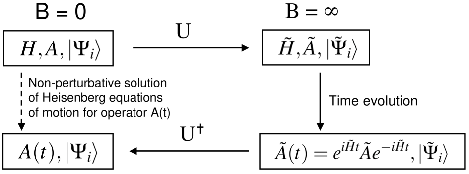
Figure 1: The forward-backward transformation scheme induces a non-perturbative solution to the Heisenberg equation of motion for an operator $A$. $U$ denotes the full unitary transformation that relates the $B=0$ to the $B=\infty$ basis hackl08a .

Intuitively, the basis defined by constructing the non-interacting normal form of the Hamiltonian should be much more suitable to solve Heisenberg’s equation of motion. This has been used in numerous examples for evaluating equilibrium correlation functions on all energy scales using flow equations KehreinBook . At the same time it also allows the calculation of nonequilibrium real-time evolution problems. Indeed, the analogy of constructing normal forms of interacting Hamilton functions in order to integrate Hamilton’s equation of motion is a very successful concept in classical mechanics, known as “canonical perturbation theory” goldstein02 . Based on the flow equation approach, this idea can be directly applied to quantum many-body systems hackl08a ; hackl09c . The general setup is described by the diagram in Fig. 1, where $|\Psi_{i}\rangle$ is some initial non-thermal state whose time evolution one is interested in. Here and in the following, we describe operators and coupling constants in the $B=\infty$ basis by a tilde. In order to study the real-time evolution of a given observable $A$ that one is interested in, the observable is transformed into the diagonal basis by solving the differential equation

$$\frac{dO}{dB}=[\eta(B),O(B)]$$ (4)

with the initial condition $O(B=0)=A$. The key observation is that one can now solve the real-time evolution with respect to the energy-diagonal $\tilde{H}$ exactly, thereby avoiding any errors that grow proportional to time (i.e. secular terms): this yields $\tilde{A}(t)$. Now since the initial quantum state is given in the $B=0$ basis, one undoes the basis change by integrating Eq. (4) from $B=\infty$ to $B=0$ (backward transformation) with the initial condition $O(B=\infty)=\tilde{A}(t)$. One therefore effectively generates a new non-perturbative scheme for solving the Heisenberg equation of motion for an operator, $A(t)=e^{iHt}A(0)e^{-iHt}$, in exact analogy to canonical perturbation theory. In a first successful application, this approach has been applied to dissipative quantum systems hackl09c ; hackl08a . In this paper, we will discuss recent work on the ferromagnetic Kondo model (Sec. 3), the fermionic Hubbard model (Sec. 4) and on steady state transport through Kondo dots (Sec. 5).

Usually, the implementation of the flow equation approach relies on approximations that allow to truncate the hierarchy of flowing interaction terms generated during the transformation of an interacting many-particle Hamiltonian and all observables. Systems that are accessible by perturbative RG are ideally suited for that purpose, since they allow for a controlled expansion around a weak-coupling fixed point.

3 Ferromagnetic Kondo model

A well-known example for a weak-coupling many-particle system can be realized in the ferromagnetic regime of the Kondo model

$$H=\sum_{\bm{k}\sigma}\varepsilon_{\bm{k}}c_{\bm{k}\sigma}^{\dagger}c_{\bm{k}\sigma}^{\phantom{\dagger}}+\sum_{\bm{k},\bm{k}^{\prime}}J_{\bm{k}^{\prime}\bm{k}}^{\parallel}S^{z}s_{\bm{k}^{\prime}\bm{k}}^{z}+\sum_{\bm{k},\bm{k}^{\prime}}J_{\bm{k}^{\prime}\bm{k}}^{\perp}(S^{+}s_{\bm{k}^{\prime}\bm{k}}^{-}+S^{-}s_{\bm{k}^{\prime}\bm{k}}^{+})\ ,$$ (5)

where $S^{\pm}=S^{x}\pm iS^{y}$ and likewise for the conduction electron spin densities. In the following, we consider constant ferromagnetic exchange couplings with $|J^{\perp}|\leq J^{\parallel}$. The canonical generator is immediately obtained from $\eta(B)=[H_{0},H_{\text{int}}(B)]$, where the flowing interaction $H_{\text{int}}(B)$ is parametrized by the flowing couplings $J_{\bm{k},\bm{k}^{\prime}}^{\parallel}(B)$ and $J_{\bm{k},\bm{k}^{\prime}}^{\perp}(B)$. At the Fermi surface (with $J_{\bm{k}_{F},\bm{k}_{F}}^{\perp,\parallel}\equiv J^{\perp,\parallel}$ and the density of states $\rho$), it can be shown that these couplings reproduce the usual poor man’s scaling equations anderson70

$$\frac{dJ^{\parallel}}{d\ln\Lambda} = -\rho(J^{\perp})^{2}\ ,$$

$$\frac{dJ^{\perp}}{d\ln\Lambda} = -\rho J^{\perp}J^{\parallel}\ .$$ (6)

For ferromagnetic couplings, the non-interacting fixed point of Eq. (6) is stable and allows for a controlled perturbative expansion of all flow equations used to transform $H$ and $S^{z}$. This example allows to analytically implement the approach outlined in Sec. 2 to calculate the time-dependent impurity magnetization $\langle S^{z}(t)\rangle$ with respect to the initial state

$$|\Psi_{i}\rangle=|\uparrow\rangle\otimes|\text{FS}\rangle\ .$$ (7)

The state $|\Psi_{i}\rangle$ has the physical interpretation of an initially decoupled system of a polarized impurity spin $|\uparrow\rangle$ and a non-interacting Fermi sea in equilibrium, $|\text{FS}\rangle$. The remaining technical steps consist of transforming the operator $S^{z}$ according to Fig. 1, in order to evaluate the observable $\langle S^{z}(t)\rangle$.

The impurity magnetization is obtained as follows. It is straightforward to work out the ansatz for the flowing spin operator as

$$S^{z}(B)=h(B)S^{z}+\sum_{\bm{k}\bm{k}^{\prime}}\gamma_{\bm{k}^{\prime}\bm{k}}(B):({\bm{S}}\times{\bm{s}}_{\bm{k}^{\prime}\bm{k}})^{z}:\ .$$ (8)

In the limit $B\rightarrow\infty$, the coupling constant $h(B)$ approaches the value $h(B\rightarrow\infty)=1+\rho J/2+\mathcal{O}(J^{2})$ if $J^{\parallel}=J^{\perp}$. The value $h(B\rightarrow\infty)/2$ is equal to the equilibrium impurity magnetization in presence of an infinitesimal Zeeman term $0^{+}S^{z}$ and has been calculated to the same accuracy by Abrikosov abrikosov70 by a summation over parquet diagrams. According to our strategy for the solution of Heisenberg’s equation of motion, the nonequilibrium magnetization follows from an ansatz

$$S^{z}(B,t)=h(B,t)S^{z}+\sum_{\bm{k}\bm{k}^{\prime}}\gamma_{\bm{k}^{\prime}\bm{k}}(B,t):({\bm{S}}\times{\bm{s}}_{\bm{k}^{\prime}\bm{k}})^{z}:\ .$$ (9)

Obviously, the flow equations for this operator have the same form as the time-independent flow equations for the ansatz in Eq. (8). It is furthermore trivial to determine the initial condition as $S^{z}(B\rightarrow\infty,t)=h(B\rightarrow\infty)S^{z}+\sum_{\bm{k},\bm{k}^{\prime}}\gamma_{\bm{k}^{\prime}\bm{k}}(B\rightarrow\infty)e^{it(\varepsilon_{\bm{k}^{\prime}}-\varepsilon_{\bm{k})}}:\bigl{(}S^{+}s_{\bm{k}^{\prime}\bm{k}}^{-}+S^{-}s_{\bm{k}^{\prime}\bm{k}}^{+}\bigr{)}:\ .$ Up to neglected normal ordered terms of $\mathcal{O}(J^{2})$, the operator $S^{z}(t)$ readily follows from integrating Eq. (9) with the initial condition $S^{z}(B\rightarrow\infty,t)$. Using these steps, the formal result for the impurity magnetization reads

$$\langle S^{z}(t)\rangle=\frac{\tilde{h}}{2}+\sum_{\bm{k}\bm{k}^{\prime}}\frac{\tilde{\gamma}_{\bm{k}\bm{k^{\prime}}}^{2}}{2}\biggl{(}e^{it(\epsilon_{\bm{k}}-\epsilon_{\bm{k^{\prime}}})}-\frac{1}{2}\biggr{)}n(\bm{k^{\prime}})[1-n(\bm{k})]\ .$$ (10)

By solving the flow equations for the couplings $\tilde{\gamma}_{\bm{k}\bm{k^{\prime}}}$ for momenta close to the Fermi surface, it is therefore possible to directly obtain the long-time dynamics of the impurity magnetization. More details of the calculation can be found in Refs. hackl09a ; hackl09b . For isotropic couplings and using a flat band with the dimensionless range $[-1,1]$, this yields the asymptotic behavior

$$\langle S^{z}(t)\rangle=\frac{1}{2}\biggl{(}\frac{1}{\ln(t)-\frac{1}{\rho J}}+1+\rho J+\mathcal{O}(J^{2})\biggr{)}\ .$$ (11)

This asymptotic behavior is confirmed by numerical calculations depicted in Fig. 2. For anisotropic couplings, the calculation is completely analogous and yields the result

$$\langle S^{z}(t)\rangle=\frac{1}{2}\biggl{(}1-\frac{\alpha^{2}}{2\tilde{j}^{\parallel}}t^{2\tilde{j}^{\parallel}}+\frac{\alpha^{2}}{2\tilde{j}^{\parallel}}\biggr{)}+\mathcal{O}(J^{2})\ ,$$ (12)

with the dimensionless coupling $\tilde{j}^{\parallel}=\rho\sqrt{J^{\parallel 2}-J^{\perp 2}}$ and $\alpha\approx\rho J^{\parallel}$ for $|J^{\perp}/J^{\parallel}|\geq 2$. These results allow for two interesting observations: (i) the time-dependent contribution to $\langle S^{z}(t)\rangle$ is described by $J^{\parallel}(\Lambda=1/t)$, where $J^{\parallel}(\Lambda)$ flows according to the scaling equations. (ii) The asymptotic result $\langle S^{z}(t\rightarrow\infty)\rangle_{\Psi_{i}}-1/2=2(\langle S^{z}\rangle_{eq}-1/2)$ is obeyed. Therefore, a factor of two distinguishes the asymptotic results for the equilibrium magnetization vs. the nonequilibrium magnetization.

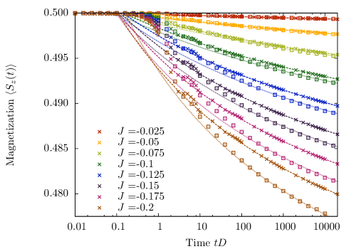
Figure 2: Time-dependent magnetization in the isotropic ferromagnetic Kondo model. $\Box$ denotes the flow equation data points, which agree very well with time-dependent numerical renormalization group calculations depicted by $\times$ hackl09b . The deviations for larger values of the coupling constant $J$ can be understood from the perturbative nature of the flow equation calculation hackl09a . Using our analytical result we fitted the flow equation data against $\langle S^{z}(t)\rangle=(1+aJ+[\ln(t)-1/(cJ)]^{-1})/2$ using $a,c$ as fit parameters (lines).

In this section we discussed a rare example where the nonequilibrium dynamics of an interacting many-particle system can be described analytically. The versatility of the flow equation approach to describe both equilibrium and nonequilibrium quantities with common scaling transformations allows to directly relate nonequilibrium relaxation laws to equilibrium properties obtained by a conventional renormalization group calculation. In our example, we could establish that nonequilibrium dynamics is set by the flowing coupling constants, evaluated at the energy scale equal to the inverse time scale of the relaxation process. Furthermore, we could show that an equilibrium and a corresponding nonequilibrium observable in a steady state differ by a factor of two. This observation appears in a much wider class of problems, e.g. in a class of discrete models, where this result can be stated in form of a theorem moeckel09 . The same factor two also appears for the real-time evolution in the weak coupling phase of the quantum Sine-Gordon model Sabio , where it connects the equilibrium with the nonequilibrium mode occupation numbers. It will be one of the central features for the real time evolution of the Hubbard model in Sec. 4 since it defines the prethermalization and ensuing thermalization behavior.

4 Small interaction quenches in the Hubbard model

The forward-backward transformation scheme as it is depicted in Fig. 1 became a fruitful tool also for examining the nonequilibrium properties of closed translation-invariant interacting quantum many-body systems. Since the trace of the squared density operator $\rho$ does not change under unitary time evolution, a closed quantum system which has been initialized in a pure state (defined by $\text{Tr}[\rho^{2}]=1$) will never relax to a thermal state (defined by $\text{Tr}[\rho^{2}]<1$). Nonetheless, the question of relaxation and thermalization can be addressed for expectation values of observables. As the conventionally studied simple observables typically only probe one- or two-particle aspects of the many-particle quantum state, there is the generic expectation that the full unitary evolution cannot be resolved; then the apparent dynamics of these observables becomes arbitrary close to that of a thermal state. This is, however, not the case for integrable models where the dynamics is limited by additional conserved integrals of motion. In the following we will show that the Hubbard model in more than one dimension, which is commonly considered nonintegrable, exhibits the phenomenon of prethermalization. It is characterized by the emergence of different relaxation times for various observables and has previously been observed numerically in cosmological models BergesPRL . This implies that there exists a transient time regime during which the expectation values of some observables have already relaxed to their long-time values while others have not. The relaxation of the latter ones, however, is only delayed to a later time scale.

We start with imposing nonequilibrium initial conditions by a quantum quench, i.e. a sudden change in a parameter of the Hamiltonian: We start in the ground state of a noninteracting Fermi gas and assume that the strength of the Hubbard interaction remains small such that we always remain within the Fermi liquid phase of the model. Therefore we first test the nonequilibrium properties of a Fermi liquid beyond Landau’s theory. Quenches outside of the Fermi liquid phase are discussed using the DMFT approach in Sec. 7. Here we apply the forward-backward scheme which allows for an analytical ab initio real-time analysis of the subsequent relaxation dynamics of the kinetic energy and the momentum distribution moeckel08 ; Moeckel2009PhD . It will turn out that the Fermi liquid picture provides a most suitable framework to understand the origin of prethermalization on the grounds of an analytical calculation. In the following paragraphs we will explain how prethermalization emerges from the interplay of the Pauli principle with quantum correlations induced by the two-particle interaction.

The time evolution of a closed many-particle quantum system is fully described by its Hamiltonian. Let us assume that the latter contains different interactions between the various degrees of freedom on well-separated energy scales, for instance a two-particle interaction between electrons, an additional electron-phonon coupling or one to an external light field. Then one trivially expects that the relaxation of a generic excited state passes through a sequence of transient time regimes: each of them corresponds to an energy scale of the Hamiltonian and exhibits its own characteristic signatures; only afterwards full thermalization of all degrees of freedom may be reached.

Prethermalization of a Fermi liquid describes a similar sequence of time regimes which originates, however, from a single two-particle interaction term in the Hamiltonian. Moreover, it is reminiscent of a common effective approach for weakly interacting systems which discusses the Hamiltonian time evolution in terms of two different relaxation mechanisms: dephasing of the initial state and two-particle scattering between unrenormalized momentum modes. This corresponds to two distinct relaxation times: short time inelastic energy relaxation and long time elastic momentum relaxation. Prethermalization implies that these time scales separate and are observable in the relaxation behavior of different observables: ’bulk’ quantities like the total kinetic or potential energy of the system are ’momentum mode averaged’ quantities which already relax due to dephasing. This can be seen as an implication of energy-time uncertainty which allows for rapid energy exchange at short times. However, in a translationally invariant system, (quasi-) momentum is conserved and the momentum distribution can only relax by momentum exchange due to scattering processes. Yet in a zero temperature Fermi liquid, scattering processes at the Fermi energy are suppressed by phase space restrictions which are imposed by the Pauli principle. Hence the momentum distribution represents the simplest example of a ’momentum mode quantity’ which relaxes on a later time scale. The separation of both time scales opens the transient regime of prethermalization during which a quasi-equilibrium description based on temperature cannot be defined for momentum mode quantities.

We develop this scenario starting from a noninteracting Fermi gas at zero temperature, i.e. in the noninteracting ground state $\left|{\Omega_{0}}\right\rangle$. Its momentum distribution exhibits a discontinuity of size $Z^{0}=1$ at the Fermi energy. Then the two-particle Hubbard interaction is switched on instantaneously,

$$H=-\sum_{\langle i,j\rangle,\sigma}t_{ij}c^{\dagger}_{i\sigma}c_{j\sigma}+U\Theta(t)(n_{i,\uparrow}-\frac{1}{2})(n_{i\downarrow}-\frac{1}{2})\ ,$$ (13)

where $c_{i}$ denotes a local fermionic destruction operator, $n_{i}=c^{\dagger}_{i}c_{i}$ the number operator in real space ($n_{k}$ in momentum space) and $\Theta(t)$ the Heaviside step function. We assume that the nearest-neighbor hopping $t_{ij}$ is larger than the local on-site two-particle interaction $U\lesssim t_{ij}\equiv 1$ to permit a weak-coupling description. The sudden change in the Hamiltonian initializes the system in a highly excited state and violates the fundamental prerequisite of Landau’s equilibrium theory of a Fermi liquid, namely the adiabatic continuity of the noninteracting and the interacting Fermi system. Nonetheless we observe that important aspects of Landau’s theory, in particular the quasiparticle picture of elementary excitations, are retained during the subsequent nonequilibrium dynamics. Applying the unitary perturbation scheme of Fig. 1 to the creation operator in momentum space implements its Heisenberg equation of motion. Thereby, it exhibits the decay of a physical fermion $c_{k}^{\dagger}$ into a superposition of various many-particle excitations which represent the ’dressing’ of the noninteracting particle with particle-hole pairs due to interaction effects,

$$c_{k\sigma}(t=0,B)\stackrel{{\scriptstyle\rm time}}{{\rightarrow}}c_{k\sigma}(t,B)=h_{k\sigma}(t,B)\ c_{k\sigma}+M_{pqr\sigma\bar{\sigma}\bar{\sigma}}(t,B)\ c_{p\sigma}^{\dagger}c_{q\bar{\sigma}}^{\dagger}c_{r\bar{\sigma}}+\ldots\ .$$ (14)

This ansatz is analog to the ansatz for the impurity magnetization (8) in the ferromagnetic Kondo model. It transfers the time evolution of operators (and/or their flow under infinitesimal unitary transformations) to a set of coupled differential flow equations for the time and $B$-dependent prefactors $h_{k\sigma}(t,B)$ and $M_{pqr\sigma\bar{\sigma}\bar{\sigma}}(t,B)$. Higher order terms are truncated in a systematic way: only terms are kept which are relevant for a second order in $U$ result of the momentum distribution function $N_{k}(t)=\left\langle{\Omega_{0}}\right|n_{k}(t)\left|{\Omega_{0}}\right\rangle$. At the Fermi surface, the coefficient $h_{k_{F}\sigma}(t)=\sqrt{Z(t)}$ relates to the time dependent value of the quasiparticle residue $Z$. The later mirrors the discontinuity of the momentum distribution function at the Fermi energy which is reduced under the time evolution. It approaches – in a formal long-time limit – a nonvanishing value $Z^{\rm NEQ}$ which mismatches the corresponding equilibrium value $Z^{\rm EQU}$ by a factor $\mu=\lim_{t\gg 1/U}(Z^{0}-Z^{\rm NEQ}(t))/(Z^{0}-Z^{\rm EQU})=2$. A comparison with exactly solvable models, e.g. the sudden squeezing of a harmonic oscillator moeckel09 , indicates that the mismatch is a nonperturbative effect of nonequilibrium dynamics, while its numerical value $\mu=2$ is a perturbative result in the weak-coupling limit. Such a mismatch is the generic behavior of many systems and observables moeckel09 . We have found it also comparing the nonequilibrium and equilibrium magnetization in the ferromagnetic Kondo model (cf. Sec. 3). For the Fermi liquid, the persistence of a nonvanishing quasiparticle residue up to late times has been confirmed recently Uhrig2009 . Hence, up to a factor the momentum distribution still resembles that of a zero temperature Fermi liquid in equilibrium; therefore we conclude that a quasiparticle picture remains applicable. Note that, due to the mismatch, the corresponding quasiparticle momentum distribution is a nonequilibrium one: deviations from a description in terms of Landau quasiparticles are second order in $U$ and open phase space for additional quasiparticle scattering. Moreover, the kinetic energy $E_{\rm kin}(t)=\int d\epsilon_{k}\epsilon_{k}N_{\epsilon_{k}}(t)$ already relaxes to its final value during this first episode of the dynamics, which is on a time scale given by $t_{1}\sim 1/\rho_{F}U^{2}$. More details of the calculation can be found in Refs. moeckel08 ; moeckel09 ; Moeckel2009PhD .

Corrections to the second order result imply a second stage of the dynamics. Motivated by the explicit calculation of one (out of many) forth order term we describe them by an effective kinetic evolution of the nonequilibrium momentum distribution using a quantum Boltzmann equation. The later describes the redistribution of occupation among quasiparticle momentum modes due to two-particle scattering events,

$$\frac{dN^{\rm QP}_{k}(t)}{dt}=\mathcal{I}_{k}[N^{\rm QP}(t)]=-U^{2}\sum_{pqr}\mathcal{P}_{kpqr}[N^{\rm QP}(t)]\delta^{k+p}_{q+r}\delta(\epsilon_{k}+\epsilon_{p}-\epsilon_{q}-\epsilon_{r})\ .$$ (15)

The scattering integral $\mathcal{I}_{k}[N^{\rm QP}(t)]$ contains the characteristic fermionic phase space factor which implements the constraints due to the Pauli exclusion principle on two-particle scattering,

$$\mathcal{P}_{kpqr}[N^{\rm QP}]=\left[N_{k}^{\rm QP}N_{p}^{\rm QP}(1-N_{q}^{\rm QP})(1-N_{r}^{\rm QP})-(1-N_{k}^{\rm QP})(1-N_{p}^{\rm QP})N_{q}^{\rm QP}N_{r}^{\rm QP}\right]\ .$$ (16)

Note that the scattering integral vanishes for arbitrary Fermi-Dirac distributions including that one of the zero temperature Fermi gas $N^{0}$. Hence a thermal state is an attractive fixed point of the Boltzmann dynamics. Since a quasiparticle picture has been established during the first stage we apply the quasiparticle momentum distribution of the transient state $N^{\rm QP}(t_{1})$ as the initial condition of the further quantum Boltzmann dynamics. Linearizing the scattering integral around $N^{0}$ and noting that the displacement $\Delta N_{k}^{\rm QP}=N^{\rm QP}(t_{1})-N^{0}$ is proportional to $U^{2}$ shows that this subsequent relaxation of the momentum distribution happens on a second time scale given by $t_{2}=1/\rho^{3}U^{4}$. For small interaction strength $t_{2}\gg t_{1}$. This delayed relaxation behavior is reminiscent of the long nonequilibrium relaxation times in glasses. Those are explained by a ragged potential landscape: local minima represent transient states which are well-separated from the global thermodynamic ground state by energy barriers. The example of the Fermi liquid shows that, in many-body quantum systems, analogue bottlenecks to the relaxation can be imposed by particle correlations. For Fermi systems at very low temperatures this is provided by the strong quantum statistical correlations due to the Pauli principle. However, this restriction is not exact, and in nonequilibrium significant quasiparticle scattering remains effective. Therefore thermalization of the momentum distribution can be expected on times $t>t_{2}$. The existence of the prethermalization regime in the Hubbard model and its subsequent relaxation has been confirmed numerically in DMFT calculations, see Sec. 7.

Prethermalization is particularly relevant in ultracold Fermi gases: There it limits the efficiency of evaporative cooling since equilibration of the remaining atoms is very slow. However, successive work has shown that this delayed thermalization may be turned into a feature and might simplify the observation of characteristic nonequilibrium physics at zero temperature, for instance nonequilibrium BCS behavior MoeckelNJP2010 .

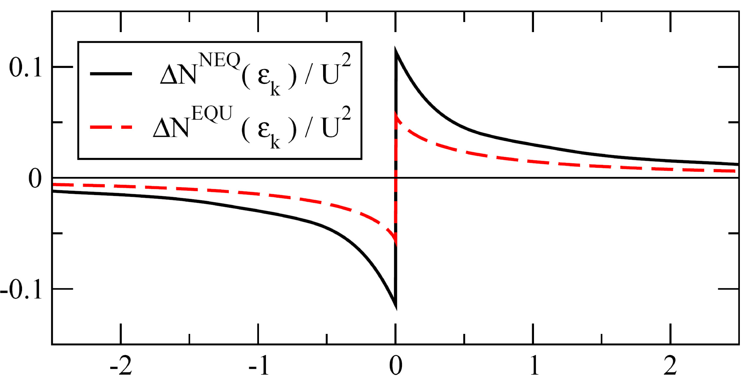
Figure 3: Comparison of correlation-induced corrections to the momentum distribution function in equilibrium (broken line) and nonequilibrium (full line). One easily reads off the twice as large reduction of the quasiparticle residue at the Fermi energy in the nonequilibrium case as compared to equilibrium.

5 Transport beyond the linear response regime through Kondo dots

A second important class of nonequilibrium problems is posed by transport beyond the linear response regime. While transport in the linear response regime essentially only probes the equilibrium ground state since the transport coefficients can be related to fluctuations in equilibrium, a correct description of the nonlinear response regime requires an understanding of the feedback of transport on the steady current-carrying state itself. In particular, many energy scales contribute to transport in this regime, which makes it conceptually difficult to access using traditional scaling techniques which focus on low-energy properties.

An experimental and theoretical paradigm for transport beyond the linear response regime is realized in Coulomb blockade quantum dots in the Kondo regime, where a voltage bias $V$ exceeding the Kondo energy scale $T_{\rm K}$ can easily be applied GoldhaberGordon ; Cronenwett ; Schmid ; vanderWiel . The key theoretical insight for understanding this situation is the observation that the shot noise of the current across the dot leads to decoherence, which suppresses the coherent many-particle processes responsible for Kondo strong coupling physics Rosch2001 .

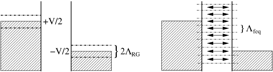
Figure 4: Left: Conventional scaling picture where states are integrated out around the two Fermi surfaces with voltage bias $V$ (here depicted for cutoff $\Lambda_{\rm RG}<V$). Right: Flow equation approach. Here all scattering processes with energy transfer $|\Delta E|\lesssim\Lambda_{\rm feq}$ are retained in $H(\Lambda_{\rm feq})$.

The flow equation method captures this physics easily since it makes the Hamiltonian successively band-diagonal as opposed to projecting on the low-energy subspace as in traditional scaling approaches. This difference is depicted in Fig. 4 for transport between two leads at different chemical potentials. Clearly, all current-carrying states continue to contribute in the flow equation scheme. It should be emphasized that there are other generalizations of conventional scaling approaches that also incorporate these processes Rosch2003 ; Rosch2005 ; Schoeller2000 ; Schoeller2009 .

Explicitly, the Kondo Hamiltonian (5) for two leads takes the following form

$$H=\sum_{a,p,\alpha}(\epsilon^{\phantom{\dagger}}_{p}-\mu^{\phantom{\dagger}}_{a})c^{\dagger}_{ap\alpha}c^{\phantom{\dagger}}_{ap\alpha}\!+\sum_{a^{\prime},a}J^{\phantom{\dagger}}_{a^{\prime}a}\sum_{p^{\prime},p}{\bm{S}}\,\cdot\,{\bm{s}}_{(a^{\prime}p^{\prime})(ap)}\ .$$ (17)

Here $a^{\prime},a=l,r$ label the two leads and the chemical potentials are given by $\mu_{l,r}=\pm V/2$. The conduction band electron spin operators are defined by ${\bm{s}}_{(a^{\prime}p^{\prime})(ap)}=\frac{1}{2}\sum_{\alpha,\beta}c^{\dagger}_{a^{\prime}p^{\prime}\alpha}{\bm{\sigma}}^{\phantom{\dagger}}_{\alpha\beta}c^{\phantom{\dagger}}_{ap\beta}$, where ${\bm{\sigma}}$ are the Pauli matrices. The couplings $J_{a^{\prime}a}$ describe the antiferromagnetic exchange interaction with the localized spin degree of freedom and are related by $J_{lr}^{2}=J^{\phantom{\dagger}}_{ll}J^{\phantom{\dagger}}_{rr}$ and $J_{ll}/J_{rr}=\Gamma_{l}/\Gamma_{r}$ if the model can be derived from an underlying Anderson impurity model. $r\stackrel{{\scriptstyle\rm def}}{{=}}\Gamma_{l}/\Gamma_{r}$ is the asymmetry parameter of the model.

The flow equation approach proceeds by using the canonical generator (3) and calculating the Hamiltonian flow (2) consistently including terms in third order of the coupling constant (details can be found in Refs. Kehrein2005 ; Fritsch2008 ; Fritsch2009 ). In equilibrium this amounts to a two loop calculation and one recovers the well-known two loop scaling equation for the coupling constant $g=\rho\,J$ at the Fermi surface

$$\frac{dg}{d\ln\Lambda_{\rm feq}}=-g^{2}+\frac{g^{3}}{2}+O(g^{4})\ .$$ (18)

The calculation is actually not different in the nonequilibrium case with voltage bias $V$ except that now normal ordering is done with respect to the shifted Fermi seas (see Fig. 4). This changes the scaling equations significantly for $\Lambda_{\rm feq}\lesssim\Gamma_{\rm rel}$ with

$$\Gamma_{\rm rel}=\sqrt{2\pi}\,\frac{V}{\ln^{2}(V/T_{\rm K})}\,\frac{1}{(1+r)(1+r^{-1})}\ ,$$ (19)

which is just proportional to the shot noise generated by the current. E.g. the scaling equation for the coupling $g_{l}$ at the Fermi surface of the left lead takes the form

$$\frac{dg_{l}}{d\ln\Lambda_{\rm feq}}=g_{l}\left(-\frac{g_{l}}{1+r^{-1}}+\frac{1}{2}\,\frac{\Gamma_{\rm rel}}{\Lambda_{\rm feq}+\Gamma_{\rm rel}}\right)\ .$$ (20)

One notices that if the coupling is not already too large at the scale $\Gamma_{\rm rel}$, then the strong coupling flow crosses over into a weak coupling flow with $g_{l}\rightarrow 0$ for $\Lambda_{\rm feq}\rightarrow 0$. This permits the controlled evaluation of physical quantities like dynamical spin susceptibility and $T$-matrix (for details see Fritsch2008 ; Fritsch2009 ). Fig. 5 for example shows the static spin susceptibility as a function of voltage bias, which crosses over quite accurately into the strong coupling equilibrium Bethe ansatz result in the limit $V\rightarrow 0$ (see inset of Fig. 5). The generalization to the case with nonvanishing magnetic field can be found in Ref. Fritsch2009 , which leads to a more intricate interplay of different decoherence scales.

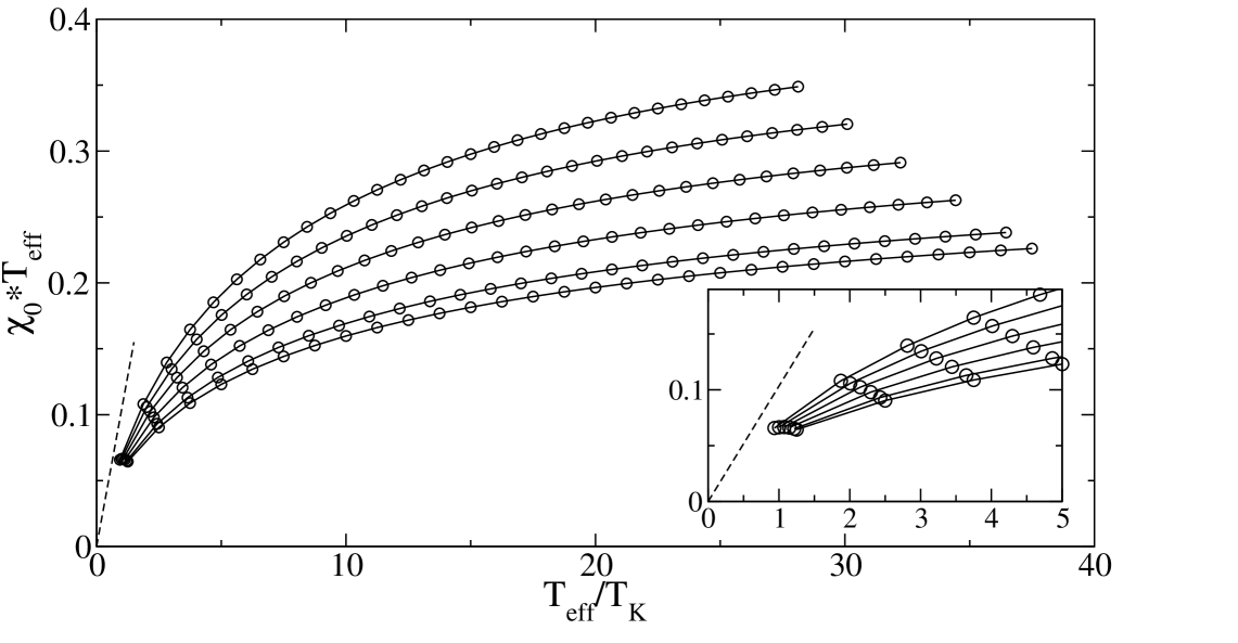
Figure 5: Flow equation results for the static spin susceptibility $\chi_{0}$ for nonzero voltage bias for various asymmetry parameters $r$ (increasing from bottom to top: $r=1.0,1.4,1.8,2.2,2.6,3.0$). The data is plotted as a function of the effective temperature $T_{\text{eff}}=V/(1+r)(1+r^{-1})$. The dashed line is an exact result for the behavior in the $T_{\rm eff}\rightarrow 0$ limit independent of asymmetry Fritsch2008 .

6 Nonequilibrium dynamical mean-field theory

Dynamical mean-field theory (DMFT) RMPGeorges usually gives a reliable description of correlated systems in equilibrium whenever their physical properties are determined by local temporal fluctuations, and spatial correlations are not too important. Within DMFT, local correlation functions of the lattice model are obtained from an effective impurity problem which contains a single site of the lattice that is coupled to a bath of noninteracting degrees of freedom. This mapping becomes exact in the limit of infinite dimensions MetznerVollhardt , and it can be formulated for both equilibrium and nonequilibrium situations Schmidt2002a , using either the imaginary-time Matsubara or the Keldysh formalism. Nonequilibrium DMFT has been used to study nonlinear transport in the Falicov-Kimball model Freericks2006a ; Freericks2008b ; Joura2008a ; Tsuji2008a ; Tsuji2009a , as well as the behavior of the Falicov-Kimball model Eckstein2008a ; Eckstein2009c and the Hubbard model Eckstein2009a when the interaction is changed abruptly, or slowly, as a function of time. Furthermore, the method can be used for the description of time-resolved photoemission Freericks2009a ; Eckstein2008c and optical spectroscopy Eckstein2008b in correlated systems.

We now briefly review the nonequilibrium DMFT formalism. A more detailed discussion of the technical aspects of this approach can be found in Refs. Freericks2006a and Eckstein2009b . We then present the derivation of a class of closed-form self-consistency equations for the nonequilibrium case. The simplest self-consistency equation results for the semi-elliptic density of states, and was used already in several studies of interaction quenches in the Falicov-Kimball Eckstein2008a ; Eckstein2009c model and the Hubbard model Eckstein2009a (cf. Sec. 7).

The impurity problem of nonequilibrium DMFT is defined via the single-site action

$$\mathcal{S}=-i\int_{\mathcal{C}}\!dt\,H_{\text{loc}}(t)-i\sum_{\sigma}\int_{\mathcal{C}}\!dt\int_{\mathcal{C}}\!dt^{\prime}\,c^{\dagger}_{\sigma}(t)\Lambda(t,t^{\prime})c_{\sigma}(t^{\prime})$$ (21)

on the Keldysh-contour $\mathcal{C}$ that runs from $t_{\text{min}}$ to some time $t_{\text{max}}$ (i.e., the largest time of interest) on the real time axis, back to $t_{\text{min}}$, and finally to $-i\beta$ along the imaginary time axis keldyshintro ; Eckstein2009b . The first term on the right-hand side of this equation contains the dynamics due to the local Hamiltonian, e.g., $H_{\text{loc}}(t)=U(t)n_{\uparrow}n_{\downarrow}-\mu(n_{\uparrow}+n_{\downarrow})$ in case of the Hubbard model with time-dependent interaction, e.g., as in Eq. (13). The second term describes the hybridization of the site with an environment that replaces the rest of the lattice, and the hybridization function $\Lambda(t,t^{\prime})$ must be determined self-consistently. From the action (21), local contour-ordered correlation functions are obtained by computing the trace $\langle A(t)B(t^{\prime})\cdots\rangle=\text{Tr}[\text{T}_{\mathcal{C}}\exp(\mathcal{S})A(t)B(t)\cdots]/Z$, where $\text{T}_{\mathcal{C}}$ is the contour-ordering operator, and real-time correlation functions can be read off from contour-ordered correlation functions by choosing the time-arguments appropriately. For the Hubbard model, the evaluation of those impurity correlation functions is the most demanding part of the DMFT solution. Real-time quantum Monte Carlo methods Werner2009a were used successfully Eckstein2009a (cf. Sec. 7), although the maximum accessible time is limited by the dynamical sign problem. On the other hand, most nonequilibrium DMFT investigations have so far been performed for the Falicov-Kimball model, where Monte Carlo methods are not needed because one can derive a closed set of equations of motion for the impurity Green functions Brandt1989a , which is then solved on the real time axis.

To determine the hybridization function $\Lambda(t,t^{\prime})$ self-consistently, one must first compute the local self-energy $\Sigma$ from the Dyson equation of the impurity model,

$$G=[i\partial_{t}+\mu-\Lambda-\Sigma]^{-1},$$ (22)

where $G(t,t^{\prime})=-i\langle\text{T}_{\mathcal{C}}c_{\sigma}(t)c_{\sigma}^{\dagger}(t^{\prime})\rangle$ is the local Green function. Here and in the following, correlation functions are matrices in their contour-time variables. Matrix multiplication denotes a convolution along the contour $\mathcal{C}$, the identity is the contour delta-function keldyshintro , and the operator $\partial_{t}$ denotes the time derivative. Furthermore, we restrict ourselves to the paramagnetic phase and omit spin indices. Because there is usually no translational invariance in time in nonequilibrium situations, Eq. (22) must be solved in the time domain instead of the frequency domain. Next, the momentum-dependent Green function $G_{{\bm{k}}}=-i\langle\text{T}_{\mathcal{C}}c_{{{\bm{k}}}\sigma}(t)c_{{{\bm{k}}}\sigma}^{\dagger}(t^{\prime})\rangle$ of the lattice model is obtained from the lattice Dyson equation

$$G_{{\bm{k}}}=[i\partial_{t}+\mu-\epsilon_{{\bm{k}}}-\Sigma]^{-1},$$ (23)

where spatial homogeneity has been assumed, and $\epsilon_{{\bm{k}}}$ are the band energies. The DMFT self-consistency is finally closed by computing the local Green function at a given site $j$ in the lattice model, $G_{j\sigma}=\sum_{{\bm{k}}}|\langle j|{{\bm{k}}}\rangle|^{2}G_{{{\bm{k}}}\sigma}$, and requiring it to be equal to the local Green function $G$ of the impurity model. If the band energies $\epsilon_{{\bm{k}}}$ are time-independent, i.e., when there is no external electrical field, the momentum summation can be reduced into a single energy integral

$$G=\int\!d\epsilon\,\rho(\epsilon)G(\epsilon),$$ (24)

where $\rho(\epsilon)=\sum_{{\bm{k}}}|\langle j|{{\bm{k}}}\rangle|^{2}\delta(\epsilon-\epsilon_{{\bm{k}}})$ is the local density of states, and $G(\epsilon_{{\bm{k}}})=G_{{\bm{k}}}$ is the momentum-dependent Green function that depends on momentum only via the band energy $\epsilon_{{\bm{k}}}$.

The numerical solution of Eqs. (22) and (23) is achieved either via an explicit matrix inversion Freericks2008b (after the contour $\mathcal{C}$ is discretized into $N$ time slices, and all contour Green functions, the derivative operator, and the identity are transformed into $N$-dimensional matrices), or the equations are rewritten as a set of integro-differential equations of Volterra type which are then solved by standard numerical algorithms Eckstein2009b . Although both approaches are rather well behaved and can be carried on to quite long times $t_{\text{max}}$ (see, e.g., Eckstein2009c ) the numerical effort can add up considerably if the ${{\bm{k}}}$ summation or $\epsilon$ integration in Eq. (24) requires a large number of ${{\bm{k}}}$-points Freericks2006a ; Freericks2008b . It is therefore desirable to find cases in which Eqs. (22)-(24) can be further simplified. Such a simplification occurs for the semi-elliptic density of states (with bandwidth $W=4$),

$$\rho(\epsilon)=\frac{\sqrt{4-\epsilon^{2}}}{2\pi},$$ (25)

which corresponds to nearest-neighbor hopping on the Bethe lattice Economou1979a ; Mahan2001a ; Eckstein2005a ; Kollar2005a , or a particular kind of long-range hopping on the hypercubic lattice Bluemer2003a . If the density of states (25) is inserted in Eq. (24), the self-energy can be eliminated from Eqs. (22)-(24), such that one obtains a closed expression for the Weiss field Eckstein2008a ,

$$\Lambda=G.$$ (26)

This closed form of the self-consistency reduces the DMFT self-consistency cycle to a repeated solution of Eq. (26) and the single-site problem for the local Green function $G$. In case of the interaction quench in the Falicov-Kimball model the existence of a closed self-consistency is crucial for the derivation of an analytical solution, thus providing the unique opportunity to study the limit of infinite times. We will now give a detailed derivation of this relation from a slightly more general statement, which in principle allows to obtain similar closed form self-consistency equations for densities of states other than Eq. (25).

Suppose that a density of states $\rho(\epsilon)$ is given and that its Hilbert transform,

$$g(z)=\int d\epsilon\,\frac{\rho(\epsilon)}{z-\epsilon},$$ (27)

for complex frequency $z$ satisfies the equation

$$zg=1+\sum_{n=1}^{\infty}f_{n}g^{n}.$$ (28)

with an analytical function $F(g)=\sum_{n=1}^{\infty}f_{n}g^{n}$ with real coefficients $f_{n}$. Note that the coefficients $f_{n}$ can be obtained order by order by first expanding Eq. (27) for large $z$ and inverting the resulting moment expansion into a series of $z$ in powers of $g$. For example, $F(g)=g^{2}$ for the semi-elliptic density of states (25).

Consider now square matrices $Z$ and $G$ that are related by

$$G =\int d\epsilon\,\rho(\epsilon)\,G(\epsilon)$$ (29)

$$G(\epsilon) =(Z-\epsilon)^{-1}.$$ (30)

Then, as we will show in the remainder of this section, the matrices $Z$ and $G$ are determined by the matrix equation

$$ZG=1+\sum_{n=1}^{\infty}f_{n}G^{n}.$$ (31)

which is analogous to the scalar equation (28). By setting $Z=i\partial_{t}+\mu-\Sigma$ we see that Eqs. (29) and (30) correspond to Eqs. (24) and (23), respectively. Equation (28) can be transformed into Eq. (22) if we multiply it with $G$ from the right and set

$$\Lambda=\sum_{n=0}^{\infty}f_{n+1}G^{n}.$$ (32)

This last equation (which reduces to Eq. (26) for $F(g)=g^{2}$) provides the desired closed form of the self-consistency equation. We note that if $F(g)$ is not a polynomial of finite degree, one can think of a suitable expansion in terms of orthogonal polynomials, e.g., Chebyshev polynomials Weisse2006a . Because orthogonal polynomial of $G$ (which involve $n$-fold convolutions) can be computed recursively, this might still be more efficient that performing the $\epsilon$ integral (24) with one matrix inversion per integration point.

To prove Eq. (31) for general square matrices, we multiply the equation $(Z-\epsilon)G(\epsilon)$ $=$ $1$ with $\rho(\epsilon)=-{\rm Im}[g(\epsilon+i0)]/\pi$, and integrate over $\epsilon$. Using Eq. (29), this yields

$$ZG=1-\frac{1}{\pi}\int d\epsilon\,\epsilon\,{\rm Im}[g(\epsilon+i0)]\,G(\epsilon).$$ (33)

Employing Eq. (28) for the scalar $g$, one can replace $\epsilon\,{\rm Im}[g(\epsilon+i0)]$ by $\text{Im}[F(g(\epsilon+i0))]$, leading to

$$ZG=1-\frac{1}{\pi}\sum_{n}f_{n}\int d\epsilon\,{\rm Im}[g(\epsilon+i0)^{n}]\,G(\epsilon).$$ (34)

It thus remains to prove that

$$G^{n}=-\frac{1}{\pi}\int d\epsilon\,{\rm Im}[g(\epsilon+i0)^{n}]G(\epsilon)$$ (35)

holds for any integer $n\geq 1$, which is done by induction: The initial step ($n=1$) follows from the definition (29). For the induction step, consider

$$(G)^{n+1} = (G)^{n}G$$

$$\stackrel{{\scriptstyle(i)}}{{=}} \frac{1}{\pi^{2}}\int d\epsilon\,d\epsilon^{\prime}\,{\rm Im}[g(\epsilon+i0)^{n}]{\rm Im}[g(\epsilon^{\prime}+i0)]\,G(\epsilon)G(\epsilon^{\prime})$$

$$\stackrel{{\scriptstyle(ii)}}{{=}} \frac{1}{\pi^{2}}\int d\epsilon\,d\epsilon^{\prime}\,{\rm Im}[g(\epsilon+i0)^{n}]{\rm Im}[g(\epsilon^{\prime}+i0)]\,G(\epsilon)\left(\frac{Z-\epsilon+\epsilon^{\prime}-Z}{\epsilon^{\prime}-\epsilon+i0}\right)G(\epsilon^{\prime})$$

$$\stackrel{{\scriptstyle(iii)}}{{=}} \frac{1}{\pi^{2}}\int d\epsilon\,d\epsilon^{\prime}\,\frac{{\rm Im}[g(\epsilon+i0)^{n}]{\rm Im}[g(\epsilon^{\prime}+i0)]}{\epsilon^{\prime}-\epsilon+i0}\,(G(\epsilon)-G(\epsilon^{\prime}))$$

$$\stackrel{{\scriptstyle(iv)}}{{=}} -\frac{1}{\pi}\int d\epsilon\,G(\epsilon)\,(g(\epsilon+i0)^{n}{\rm Im}[g(\epsilon+i0)]+{\rm Im}[g(\epsilon+i0)^{n}]g(\epsilon-i0))$$

$$= -\frac{1}{\pi}\int d\epsilon\,{\rm Im}[g(\epsilon+i0)^{n+1}]\,G(\epsilon)\ .$$

In step (i), proposition (35) is used. In (ii), the term in braces is unity, and in (iii), we use Eq. (30). To proceed to (iv) one performs one of the two energy integrals by making use of the spectral representation

$$g(z)^{n}=-\frac{1}{\pi}\int d\epsilon\frac{{\rm Im}[g(\epsilon+i0)^{n}]}{z-\epsilon}.$$ (36)

The latter holds because $g(z)^{n}$ is analytic in the upper half plane. Summing up the terms in step (iv) and using $g(\epsilon-i0)=g(\epsilon+i0)^{*}$ completes the induction, and hence the proof of the closed self-consistency equation (32).

7 Interaction quenches in the Hubbard model in DMFT

We will now discuss the relaxation dynamics of Hubbard models after a sudden change in the interaction parameter from $0$ to a finite value of $U$, see Eq. (13). Since only the dynamics of the interacting fermions is considered, but no coupling to an external bath is present, it is not immediately clear whether the system will thermalize, i.e., whether after sufficiently long times it can be described by the thermal state that is predicted by equilibrium statistical mechanics. Many models of isolated many-body systems have so far been investigated (see, e.g., Refs. Heims65 ; Girardeau1969 ; Sengupta2004a ; Rigol2006 ; Cazalilla2006a ; Rigol2007a ; Kollath2007 ; Manmana07 ; Eckstein2008a ; moeckel08 ; Kollar2008 ; Rigol2008a ; Rossini2009b ; Barmettler2009a ; Eckstein2009a , and Dziarmaga2009 for a recent review), and in fact thermalization is only rarely observed. In this section we will discuss results obtained with nonequilibrium DMFT, which show that the system can thermalize quickly for certain values of the interaction $U$ Eckstein2009a ; Eckstein2009b .

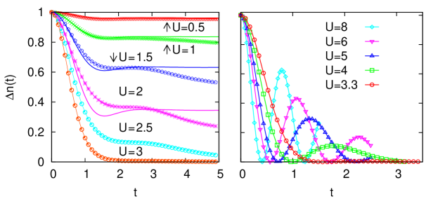
Figure 6: Fermi surface discontinuity $\Delta n$ after quenches from $U=0$ to $U\leq 3$ (left panel) and $U\geq 3.3$ (right panel) Eckstein2009a ; Eckstein2009b . The expected thermal value for this quantity is zero, corresponding to a continuous momentum distribution at finite temperature. The quarter-bandwidth $V$ is set to unity. Solid lines in the left panel indicate the flow equation prediction for the prethermalization plateau moeckel08 and the transient behavior moeckel09 for small values of $U$.

For a quench from the ground state at $U$ $=$ 0 to finite values of $U$ the DMFT equations for the paramagnetic phase (Sec. 6) were obtained in Refs. Eckstein2009a ; Eckstein2009b , using the semi-elliptic density of states (25) and real-time quantum Monte Carlo methods Werner2009a to obtain the Green function for the action (21). Fig. 6 shows the jump $\Delta n(t)$ in the momentum distribution at the Fermi surface as a function of time, in separate panels for small and large values of the final interaction parameter $U$. Clearly the time evolution after an interaction quench in the Hubbard model depends sensitively on the parameter $U$. Note that $\Delta n(t)$ remains finite for a finite time after the quench; in the case of a local self-energy as in DMFT this is due to the relation of $\Delta n(t)$ to the retarded Green function at $\epsilon=0$ Eckstein2009a . From this relation one can infer that the collapse of $\Delta n$ is closely related to the decay of charge excitations that are created at the Fermi surface by the quench. It should be noted that as long as $\Delta n(t)$ is finite the system is not yet thermalized, because a finite jump is possible in a Fermi liquid in thermal equilibrium only at zero temperature, whereas the quenched system has finite excitation energy.

For quenches to $U$ $\leq$ $3$ the Fermi surface discontinuity $\Delta n(t)$ remains finite for times $t$ $\leq$ $5$ (left panel in Fig. 6). The plateau in $\Delta n(t)$ at intermediate times is given by $2Z-1$, where $Z$ is the quasiparticle weight in equilibrium at zero temperature and interaction $U$ (cf. Sec. 4). On the other hand, the double occupation does essentially relax to its thermal value on this timescale Eckstein2009a , confirming that the potential energy (and therefore also the kinetic energy) relax quickly, whereas the occupation of individual states still changes. Interestingly the prethermalization plateau remains well visible even for quenches to relatively large $U\lesssim 2.5$, even though the timescales $V/U^{2}$ and $V^{3}/U^{4}$ are then no longer well separated. Not only the prethermalization plateaus, but also the transient behavior predicted from the flow equation analysis moeckel09 agrees well with the numerical DMFT results for $U\lesssim 1.5$. The prethermalization plateaus for small $U$ are due to the vicinity of the integrable point at $U=0$, as discussed further below.

The relaxation dynamics show different characteristics for quenches to large $U$ (right panel of Fig. 6), namely so-called collapse-and-revival oscillations with approximate frequency $2\pi/U$. These are to due the vicinity of the atomic limit ($V$ $=$ $0$), for which the propagator $e^{-iHt}$ is periodic with period $2\pi/U$-periodic Greiner . For finite $V$ these oscillations are damped and decay on timescales of order $1/V$. For the double occupation these oscillations are not centered around the thermal value, but rather around a different value that can be explained using perturbation theory for strong coupling Eckstein2009a . Somewhat analogously to the situation at small coupling the relaxation to the thermal state is thus delayed because the system is trapped in a metastable state close to an integrable point.

Interestingly both the weak-coupling prethermalization plateau in $\Delta n(t)$ and the strong-coupling oscillations disappear in a small region of interaction parameters around $U_{c}^{\text{dyn}}\approx 3.2$ Eckstein2009a . For quenches to values of $U$ near $U_{c}^{\text{dyn}}$ the system thermalizes very quickly. Not only the Fermi surface discontinuity and the double occupation relax to their thermal values, but in fact the retarded nonequilibrium Green function relaxes to the corresponding equilibrium quantity Eckstein2009b . It is therefore justified to say that the system indeed thermalizes in this case, because a large set of observables tend to the thermal value predicted by equilibrium statistical mechanics. Note that the statistical theory contains no adjustable parameter, because the effective temperature $T^{*}$ is determined by the energy of the system after the quench, for example $T^{*}=0.84$ for the quench to $U=3.3$. The sharp crossover in the relaxation parameter is intriguing, not least because the relation to the equilibrium Mott metal-insulator transition is not obvious. The critical endpoint of the latter is located at $T_{c}\approx 0.055V$ RMPGeorges , so that little of it is visible at the much higher temperatures $T^{*}$. For quenches of the anisotropy parameter in Heisenberg chains a remarkably similar behavior was found Barmettler2009a . There the staggered magnetization indeed relaxes fastest to zero for quenches to the equilibrium critical value.

It follows from these results that an isolated fermionic many-body system can thermalize merely under the time evolution with the interacting Hamiltonian, without requiring coupling to a bath. In the vicinity of an intermediate value $U_{c}^{\text{dyn}}$ the system quickly thermalizes, but for smaller or larger coupling thermalization has not been observed numerically for the short available observation times.

8 Interaction quenches in the $1/r$ Hubbard chain

For comparison we now discuss results for the one-dimensional $1/r$ Hubbard model, which was originally proposed and solved by Gebhard and Ruckenstein Gebhard92 . Its hopping amplitudes are given by $t_{mj}$ $=$ $(-iW/2L)(-1)^{m-j}/\sin[\pi(m-j)/L]$ with periodic boundary conditions, leading to a linear dispersion $\epsilon_{k}$=$Wk/(2\pi)$, where $W(=1)$ is the bandwidth. For $U$ $\geq$ $-1$ this model can be mapped to an effective free Hamiltonian for hard-core bosons Gebhard92 ; Gebhard94b for which the spectrum can be determined at once. For half-filling a Mott-Hubbard metal-insulator transition occurs at the interaction strength $U_{c}=1$ in this model, and the Mott gap is $\Delta=U-U_{c}$ in the insulating phase.

Based on this solution, the exact time evolution was obtained in Ref. Kollar2008 for a quench from $U=0$ (or $U=\infty$) to a finite value of $U$. For the quench from $U=0$ to finite $U$ at half-filling the double occupation has the noninteracting value $\frac{1}{4}$ at time $t=0$ and relaxes to a new constant value with algebraic decay,

$$d(t) =\frac{1}{8}-\frac{(1-U)^{2}}{16U}-\frac{(1-U^{2})^{2}}{16U^{2}}\ln\Big{|}\frac{1-U}{1+U}\Big{|}-\frac{\cos(Ut)\cos(t)}{2Ut^{2}}+O\Big{(}\frac{1}{t^{3}}\Big{)}\,.$$ (37)

In general the long-time limit of $d(t)$ does not agree with the thermal prediction $d_{\text{therm}}$. For example, for quenches to the critical value $U_{c}=1$ the stationary value is $d(t=\infty)=0.125$, and this differs too from the thermal prediction $d_{\text{therm}}=0.098$ that is obtained from equilibrium results Gebhard92 at the temperature that gives the same mean energy as the time-evolved state.

The reason for the nonthermal steady state in this model lies in its integrability. The interacting fermionic Hamiltonian $H$ can be mapped on an effective Hamiltonian without interactions, i.e.,

$$H=\sum_{\alpha}\epsilon_{\alpha}\;{\cal I}_{\alpha}\,,$$ (38)

where the ${\cal I}_{\alpha}$ have the eigenvalues 0 or 1 and commute with each other (and hence with $H$). This is a rather strong case of integrability, because not only are there many constants of motion (their number is proportional to the system size), but also the energy levels can be populated independently (unlike, e.g., in many other models that can be solved by Bethe ansatz). As a consequence the fundamental postulate of statistical mechanics is not fulfilled, which states that all accessible microstates are assumed to be equally probable in the ensemble description of the equilibrium state. For an integrable system (38), however, all the ${\cal I}_{\alpha}$ remain at their values in the initial state at $t=0$. That this restriction leads to nonthermal steady states has been observed in a variety of models Girardeau1969 ; Sengupta2004a ; Rigol2006 ; Cazalilla2006a ; Rigol2007a ; Manmana07 ; Eckstein2008a , and also in experiments with cold atomic gases Kinoshita2006a .

9 Statistical description of nonthermal steady states with generalized Gibbs ensembles

As described in the previous subsection, standard statistical mechanics cannot be expected to predict the steady state after a quench in an integrable system correctly. This leads to the question whether a suitably generalized statistical theory can make the correct prediction. The general procedure to construct the statistical operator in statistical mechanics is to maximize the entropy, and to take conserved quantities into account by fixing them on average using Lagrange multipliers Balian91a . This means that for the integrable Hamiltonian (38) all constants of motion ${\cal I}_{\alpha}$ should be fixed on average such that they yield the correct initial expectation value Rigol2006 ; Rigol2007a , leading to a generalized Gibbs ensemble (GGE)

$$\rho_{\text{GGE}} \propto e^{-\sum_{\alpha}\lambda_{\alpha}{\cal I}_{\alpha}}\,,$$ (39)

with $\lambda_{\alpha}$ determined from $\langle{\cal I}_{\alpha}\rangle_{\text{GGE}}=\langle{\cal I}_{\alpha}\rangle_{0}$. For the $1/r$ Hubbard chain discussed in the previous subsection, the GGE prediction for the stationary value of the double occupation agrees precisely with the calculated long-time limit Kollar2008 . However, GGEs have been found to fail for some observables in other models Rigol2006 .

It is possible to formulate sufficient criteria for the steady state to be correctly described by the ensemble (39). In general this depends on both the initial state $\left|{\psi(t=0)}\right\rangle$ and the observable $A$ Kollar2008 . The long-time average of $\left\langle{\psi(t)}\right|A\left|{\psi(t)}\right\rangle$ is given by

$$\overline{\langle A\rangle} =\sum_{\bm{m}}\left\langle{\bm{m}}\right|A\left|{\bm{m}}\right\rangle|\left\langle{\bm{m}}|{\Psi(t=0)}\right\rangle|^{2}\,,$$ (40)

provided that the spectrum of $H$ is nondegenerate. Note that $\overline{\langle A\rangle}$ equals the long-time limit of $\langle A\rangle$, if the latter exists. Here the eigenbasis of the constants of motion, ${\cal I}_{\alpha}\left|{\bm{m}}\right\rangle$ $=$ $m_{\alpha}\left|{\bm{m}}\right\rangle$, was used. Let us assume that the constants of motion only have eigenvalue $m_{\alpha}=0,1$ and can be represented as bosons or fermions according to ${\cal I}_{\alpha}=a_{\alpha}^{\dagger}a_{\alpha}^{\phantom{{\dagger}}}$ (cf. Kollar2008 for a more general case)). Consider then an observable $A$ that can be written as a linear combination of products of $n$ creation operators $a_{\alpha_{i}}^{\dagger}$ followed by $n$ annihilation operators $a_{\alpha_{j}}^{\phantom{{\dagger}}}$. The long-time average $\overline{\langle A\rangle}$ is given by a linear combination of expectation values $\langle{\prod_{i=1}^{n}{\cal I}_{\alpha_{i}}}\rangle_{t=0}$ in the initial state; off-diagonal terms drop out due to the diagonal character of (40). On the other hand the GGE expectation value decouples each constant of motion from the others and instead involves $\prod_{i=1}^{n}\langle{{\cal I}_{\alpha_{i}}}\rangle_{t=0}$, where the condition on the parameters $\lambda_{\alpha}$ has been used. If the expectation value of the product equals the product of these expectation values for each $\alpha_{i}$ that occurs in the observable $A$, then the GGE is guaranteed to describe the expectation value of $A$ in the steady state correctly.

We see that for the GGE prediction to be correct, the ${\cal I}_{\alpha_{i}}$ that occur in $A$ must in a certain sense not be too correlated in the initial state, so that the expectation value of their product factorizes. Unfortunately the physical meaning of this condition is not obvious and certainly depends on the way in which the original degrees of freedom appear in the constants of motion. Nevertheless the GGE is certain to work for quadratic operators $a_{\alpha}^{\dagger}a_{\beta}^{\phantom{{\dagger}}}$, and this is the reason why the GGE succeeds for the double occupation in the $1/r$ Hubbard model, which can be expressed precisely as a sum of such quadratic operators Gebhard94b .

In any case we can conclude that statistical mechanics, when applied properly, does indeed predict the steady state of an integrable many-body system that is isolated and not coupled to any baths. The fact that GGEs cannot describe all expectation values correctly is actually not surprising. Even standard statistical mechanics fails for the expectation values of specially crafted operators, such as powers of the Hamiltonian or projectors onto energy eigenstates, which remain at their initial values and thus never thermalize. But these observables are typically highly nonlocal and their expectation values correspond to correlation functions of very high order. Since they are essentially impossible to measure they are not of practical importance, implying no severe limitation on the applicability of equilibrium statistical mechanics.

So far we have discussed integrable systems in the sense of Eq. (38), i.e., systems of interacting particles whose Hamiltonian can be transformed into a basis in which the new effective degrees of freedom are noninteracting, and their occupation numbers are thus constants of motion. However, any noninteracting Hamiltonian is of course also integrable, e.g., the Hubbard model with $U=0$, $H_{0}=\sum_{\bm{k}\sigma}\varepsilon_{\bm{k}}c^{{\dagger}}_{\bm{k}\sigma}c^{\phantom{{\dagger}}}_{\bm{k}\sigma}$. In this case the conserved momentum occupation numbers $c^{{\dagger}}_{\bm{k}\sigma}c^{\phantom{{\dagger}}}_{\bm{k}\sigma}$ play the role of the conserved ${\cal I}_{\alpha}$, so that thermalization is impossible when quenching to $H_{0}$.

Moreover, noninteracting Hamiltonians of course also provide useful starting points for interaction quenches, as used in Sec. 4. As discussed there, a quench to a small value of the interaction parameter will lead to prethermalization on an intermediate time scale moeckel08 , which is due the vicinity of the integrable point at $U=0$. In fact, the prethermalized expectation value of an observable $A$ can be obtained by using perturbation theory and taking the long-time limit (provided $[A,H_{0}]=0$) moeckel09 . It is therefore useful to view the prethermalization plateau as due to the conservation of certain perturbed constants of motion $\widetilde{{\cal I}}_{\alpha}$, which hinder thermalization on intermediate time scales. It is then possible to construct a generalized Gibbs ensemble $\widetilde{\rho}_{\text{GGE}}$ based on these perturbatively conserved quantities, which predicts a stationary value that agrees precisely with the long-time limit in second order perturbation theory, provided certain factorization conditions are fulfilled Kollar2010 . Namely, for an observable $A=\prod_{i}{\cal I}_{\alpha_{i}}$ the prethermalization plateau, which occurs for small quenches away from $H_{0}$, is correctly predicted by $\widetilde{\rho}_{\text{GGE}}$ if $\langle\prod_{i}{\cal I}_{\alpha_{i}}\rangle$ = $\prod_{i}\langle{\cal I}_{\alpha_{i}}\rangle$. Here the expectation value is to be taken in the (perturbed) eigenstate after the quench. Again it is not surprising to see that only sufficiently simple observables can be expected to be correctly predicted by the statistical theory. In the simplest case, the GGE prediction for the prethermalization plateau is correct for the observables ${\cal I}_{\alpha}$, e.g., the momentum distribution for quenches to small $U$ in the Hubbard model. The agreement between the time-evolved state and the GGE prediction shows that prethermalization plateaus evolve continuously from the nonthermal steady state in integrable models, at least perturbatively.

10 Conclusion

For the investigation of the nonequilibrium behavior of correlated systems robust theoretical techniques are required, because both the interaction between particles and the time evolution for sufficiently long times must be described reliably. On the one hand, we discussed the flow equation approach and its applications to isolated many-body systems in nonequilibrium such as the ferromagnetic Kondo model and the Hubbard model at weak coupling, as well as nonlinear transport through Kondo dots. This method has the advantage that the emergence of time and energy scales is explicit and transparent. For example, for small interaction quenches in Hubbard models the method reveals that the system prethermalizes, i.e., that nonthermal states form on an intermediate time scale. Quantum Boltzmann dynamics then shows that these nonthermal states thermalize on a longer time scale moeckel08 ; moeckel09 . On the other hand, we discussed applications of nonequilibrium dynamical-mean field theory, which maps a lattice system onto an effective single-site problem that can be solved numerically. The numerical results for interaction quenches in the Hubbard model confirm the prethermalization scenario and also show that thermalization can indeed occur on short timescales in an isolated many-body system at intermediate coupling. We compared with results for special solvable models, in which nonthermal steady states occur due to the presence of many constants of motion. Within second order perturbation theory, the statistical predictions of generalized Gibbs ensembles, which take these constants of motion into account, show that prethermalization in nonintegrable systems and nonthermal states in integrable systems can be related.

We thank M. Rigol for useful discussions. Financial support by the SFB 484 and TTR 80 of the Deutsche Forschungsgemeinschaft (DFG) is gratefully acknowledged. A.H. acknowledges additional support through SFB 608 and financial support through SFB/TR 12 of the DFG. S.K. and M.M. acknowledge additional support through SFB 631, SFB/TR 12, the Center for NanoScience (CeNS) Munich, and the German Excellence Initiative via the Nanosystems Initiative Munich (NIM).

References

- (1) K. G. Wilson, Rev. Mod. Phys. 47, 773 (1975)
- (2) W. Metzner, D. Vollhardt, Phys. Rev. Lett. 62, 324 (1989)
- (3) A. Georges, G. Kotliar, W. Krauth, M. J. Rozenberg, Rev. Mod. Phys. 68, 13 (1996)
- (4) M. Greiner, O. Mandel, T. W. Hänsch, I. Bloch, Nature 419, 51 (2002)
- (5) S. Iwai, M. Ono, A. Maeda, H. Matsuzaki, H. Kishida, H. Okamoto, Y. Tokura, Phys. Rev. Lett. 91, 057401 (2003)
- (6) L. Perfetti, P. A. Loukakos, M. Lisowski, U. Bovensiepen, H. Berger, S. Biermann, P. S. Cornaglia, A. Georges, M. Wolf, Phys. Rev. Lett. 97, 067402 (2006); L. Perfetti, P. A. Loukakos, M. Lisowski, U. Bovensiepen, M. Wolf, H. Berger, S. Biermann, A. Georges, New J. Phys. 10, 053019 (2008)
- (7) Y. Kawakami, S. Iwai, T. Fukatsu, M. Miura, N. Yoneyama, T. Sasaki, N. Kobayashi, Phys. Rev. Lett. 103, 066403 (2009)
- (8) S. Wall, D. Brida, S. R. Clark, H. P. Ehrke, D. Jaksch, A. Ardavan, S. Bonora, H. Uemura, Y. Takahashi, T. Hasegawa, H. Okamoto, G. Cerullo, A. Cavalleri, arXiv:0910.3808
- (9) D. Goldhaber-Gordon, H. Shtrikman, D. Mahalu, D. Abusch-Magder, U. Meirav, M. A. Kastner, Nature 391, 156 (1998)
- (10) S. M. Cronenwett, T. H. Oosterkamp, L. P. Kouwenhoven, Science 281, 540 (1998)
- (11) J. Schmid, J. Weis, K. Eberl, K. v. Klitzing, Physica B: Cond. Matt. 256-258, 182 (1998)
- (12) W. G. van der Wiel, W. De Franceschi, T. Fujisawa, J. M. Elzerman, S. Tarucha, L. P. Kouwenhoven, Science 289, 2105 (2000)
- (13) F. Wegner, Ann. Phys. (Leipzig) 3, 77 (1994)
- (14) S. Kehrein, The Flow Equation Approach to Many-Particle Systems, Springer Verlag (2006)
- (15) P. Schmidt, H. Monien, arXiv:cond-mat/0202046
- (16) J. K. Freericks, V. M. Turkowski, V. Zlatić, Phys. Rev. Lett. 97, 266408 (2006)
- (17) A. Hackl, D. Roosen, S. Kehrein, W. Hofstetter, Phys. Rev. Lett. 102, 196601 (2009)
- (18) S. D. Głazek, K. G. Wilson, Phys. Rev. D 48, 5863 (1993)
- (19) S. D. Głazek, K. G. Wilson, Phys. Rev. D 49, 4214 (1994)
- (20) A. Hackl, S. Kehrein, Phys. Rev. B 78, 092303 (2008)
- (21) H. Goldstein, Ch. P. Poole, J. L. Safko, Classical Mechanics, Third edition (Addison-Wesley, 2002), p. 526
- (22) A. Hackl, S. Kehrein, J. Phys. C 21, 015601 (2009)
- (23) P. Anderson, J. Phys. C 3, 2436 (1970)
- (24) A. Abrikosov, A. A. Migdal, J. Low Temp. Phys. 3, 519 (1970)
- (25) A. Hackl, S. Kehrein, M. Vojta, Phys. Rev. B 80, 195117 (2009)
- (26) M. Moeckel, S. Kehrein, Ann. Phys. 324, 2146 (2009)
- (27) J. Sabio, S. Kehrein, arXiv:0911.1302, to appear in New J. Phys.
- (28) J. Berges, Sz. Borsanyi, C. Wetterich, Phys. Rev. Lett. 93, 142002 (2004)
- (29) M. Moeckel, S. Kehrein, Phys. Rev. Lett. 100, 175702 (2008)
- (30) M. Moeckel, Real-time evolution of quenched quantum systems, PhD thesis (LMU München 2009).
- (31) G. S. Uhrig, Phys. Rev. A 80, 061602(R) (2009)
- (32) M. Moeckel, S. Kehrein, arXiv:0911.0875, to appear in New J. Phys.
- (33) A. Rosch, J. Kroha, P. Wölfle, Phys. Rev. Lett. 87, 156802 (2001)
- (34) A. Rosch, J. Paaske, P. Wölfle, Phys. Rev. Lett. 90, 076804 (2003)
- (35) A. Rosch, J. Paaske, J. Kroha, P. Wölfle, J. Phys. Soc. Jpn. 74, 118 (2005)
- (36) H. Schoeller, Lect. Notes Phys. 544, 137 (2000)
- (37) H. Schoeller, F. Reininghaus, Phys. Rev. B 80, 045117 (2009); Phys. Rev. B 80, 209901(E) (2009)
- (38) S. Kehrein, Phys. Rev. Lett. 95, 056602 (2005)
- (39) P. Fritsch, S. Kehrein, Ann. Phys. 324, 1105 (2009)
- (40) P. Fritsch, S. Kehrein, Phys. Rev. B 81, 035113 (2010)
- (41) J. K. Freericks, Phys. Rev. B 77, 075109 (2008)
- (42) A. V. Joura, J. K. Freericks, T. Pruschke, Phys. Rev. Lett. 101, 196401 (2008)
- (43) N. Tsuji, T. Oka, H. Aoki, Phys. Rev. B 78, 235124 (2008)
- (44) N. Tsuji, T. Oka, H. Aoki, Phys. Rev. Lett. 103, 047403 (2009)
- (45) M. Eckstein, M. Kollar, Phys. Rev. Lett. 100, 120404 (2008)
- (46) M. Eckstein, M. Kollar, arXiv:0911.1282, to appear in New J. Phys.
- (47) M. Eckstein, M. Kollar, P. Werner, Phys. Rev. Lett. 103, 056403 (2009)
- (48) J. K. Freericks, H. R. Krishnamurthy, T. Pruschke, Phys. Rev. Lett. 102, 136401 (2009)
- (49) M. Eckstein, M. Kollar, Phys. Rev. B 78, 245113 (2008)
- (50) M. Eckstein, M. Kollar, Phys. Rev. B 78, 205119 (2008)
- (51) M. Eckstein, M. Kollar, P. Werner, Phys. Rev. B 81, 115131 (2010)
- (52) For an introduction into the Keldysh formalism, see R. van Leeuwen, N. E. Dahlen, G. Stefanucci, C.-O. Almbladh, U. von Barth, arXiv:cond-mat/0506130 (published in: Time-dependent density functional theory, M. A. L. Marques, C. A. Ullrich, F. Nogueira, A. Rubio, K. Burke, E. K. U. Gross (eds.), Lecture Notes in Physics 706, Springer, Berlin 2006)
- (53) P. Werner, T. Oka, A. J. Millis, Phys. Rev. B 79, 035320 (2009)
- (54) U. Brandt, C. Mielsch, Z. Phys. B: Condens. Matter 75, 365 (1989)
- (55) E. N. Economou, Green’s Functions in Quantum Physics, Springer-Verlag, Berlin, 1979
- (56) G. D. Mahan, Phys. Rev. B 63, 155110 (2001)
- (57) M. Eckstein, M. Kollar, K. Byczuk, D. Vollhardt, Phys. Rev. B 71, 235119 (2005)
- (58) M. Kollar, M. Eckstein, K. Byczuk, N. Blümer, P. van Dongen, M. H. R. de Cuba, W. Metzner, D. Tanasković, V. Dobrosavljević, G. Kotliar, D. Vollhardt, Ann. Phys. 14 (2005)
- (59) N. Blümer, P. G. J. van Dongen, Transport properties of correlated electrons in high dimensions, in Concepts in Electron Correlation, edited by A. C. Hewson and V. Zlatić, NATO Science Series, Kluwer, 2003.
- (60) A. Weisse, G. Wellein, A. Alvermann, H. Fehske, Rev. Mod. Phys. 78, 275 (2006)
- (61) S. P. Heims, Am. J. Phys. 33, 722 (1965)
- (62) M. D. Girardeau, Phys. Lett. A 30, 442 (1969)
- (63) K. Sengupta, S. Powell, S. Sachdev, Phys. Rev. A 69, 053616 (2004)
- (64) M. Rigol, A. Muramatsu, M. Olshanii, Phys. Rev. A 74, 053616 (2006)
- (65) M. A. Cazalilla, Phys. Rev. Lett. 97, 156403 (2006)
- (66) M. Rigol, V. Dunjko, V. Yurovsky, M. Olshanii, Phys. Rev. Lett. 98, 050405 (2007)
- (67) C. Kollath, A. Läuchli, E. Altman, Phys. Rev. Lett. 98, 180601 (2007)
- (68) S. R. Manmana, S. Wessel, R. M. Noack, A. Muramatsu, Phys. Rev. Lett. 98, 210405 (2007)
- (69) M. Kollar, M. Eckstein, Phys. Rev. A 78, 013626 (2008)
- (70) M. Rigol, V. Dunjko, M. Olshanii, Nature 452, 854 (2008)
- (71) D. Rossini, A. Silva, G. Mussardo, G. E. Santoro, Phys. Rev. Lett. 102, 127204 (2009)
- (72) P. Barmettler, M. Punk, V. Gritsev, E. Demler, E. Altman, Phys. Rev. Lett. 102, 130603 (2009)
- (73) J. Dziarmaga, arXiv:0912.4034
- (74) F. Gebhard, A. E. Ruckenstein, Phys. Rev. Lett. 68, 244 (1992)
- (75) F. Gebhard, A. Girndt, A. E. Ruckenstein, Phys. Rev. B 49, 10926 (1994)
- (76) T. Kinoshita, T. Wenger, D. S. Weiss, Nature 440, 900 (2006)
- (77) R. Balian, From Microphysics to Macrophysics: Methods and Applications of Statistical Physics, Vol. 1 (Springer, Berlin, 1991)
- (78) M. Kollar, F. A. Wolf, M. Eckstein, to be published