Dissertation
submitted to the
Combined Faculties of the Natural Sciences and Mathematics
of the Ruperto-Carola-University of Heidelberg, Germany
for the degree of
Doctor of Natural Science
Put forward by

Diplom-Physikerin Eva Meyer

born in: Essen, Germany
Oral Examination: 21st July 2010

    High Precision Astrometry with Adaptive Optics aided Imaging
   

Referees:              Prof. Dr. Hans-Walter Rix
                                Prof. Dr. Joachim Wambsganß

Abstract

Currently more than 450 exoplanets are known and this number increases nearly every day. Only a few constraints on their orbital parameters and physical characteristics can be determined, as most exoplanets are detected indirectly and one should therefore refer to them as exoplanet candidates. Measuring the astrometric signal of a planet or low mass companion by means of measuring the wobble of the host star yields the full set of orbital parameters. With this information the true masses of the planet candidates can be determined, making it possible to establish the candidates as real exoplanets, brown dwarfs or low mass stars. In the context of this thesis, an M-dwarf star with a brown dwarf candidate companion, discovered by radial velocity measurements, was observed within an astrometric monitoring program to detect the astrometric signal. Ground based adaptive optics aided imaging with the ESO/NACO instrument was used with the aim to establish its true nature (brown dwarf vs. star) and to investigate the prospects of this technique for exoplanet detection. The astrometric corrections necessary to perform high precision astrometry are described and their contribution to the overall precision is investigated. Due to large uncertainties in the pixel-scale and the orientation of the detector, no detection of the astrometric orbit signal was possible.
The image quality of ground-based telescopes is limited by the turbulence in Earth’s atmosphere. The induced distortions of the light can be measured and corrected with the adaptive optics technique and nearly diffraction limited performance can be achieved. However, the correction is only useful within a small angle around the guide star in single guide star measurements. The novel correction technique of multi conjugated adaptive optics uses several guide stars to correct a larger field of view. The VLT/MAD instrument was built to demonstrate this technique. Observations with MAD are analyzed in terms of astrometric precision in this work. Two sets of data are compared, which were obtained in different correction modes: pure ground layer correction and full multi conjugated correction.

Zusammenfassung

Mehr als 450 extrasolare Planets sind zurzeit bekannt und diese Zahl wird fast täglich grösser. Da die meisten Exoplaneten indirekt entdeckt werden, können nur wenige Einschränkungen bezüglich ihrer Bahnparameter und physikalischen Eigenschaften gemacht werden und sie sollten daher vorläufig als Exoplanet-Kandidaten bezeichnet werden. Misst man das astrometrische Signal eines planetaren oder massearmen Begleiters, indem man die Reflexbewegung des Hauptsterns vermisst, so erhält man den vollen Satz an orbitalen Parametern. Mit dieser Information kann die genaue Masse der Kandidaten bestimmt werden und es ist somit möglich, die Planetenkandidaten als wahre Exoplaneten, Braune Zwerge oder massearme Sterne einzustufen. Im Rahmen der vorliegenden Doktorarbeit wurde ein Zwergstern der Spektralklasse M, der einen mittels Radialgeschwindigkeitsmessungen entdeckten wahrscheinlichen Braunen Zwerg als Begleiter hat, innerhalb eines fortlaufenden Beobachtungsprogramms zur Detektion des astrometrischen Signals beobachtet. Bodengebundene Beobachtungen mit dem Adaptiven Optik (AO) Instrument ESO/NACO wurden durchgeführt, um die wahre Natur des Begleiters zu bestimmen (Brauner Zwerg oder massearmer Stern) und die Aussichten dieser Technik im Bereich der Planetenendeckung zu untersuchen. Die astrometrischen Korrekturen, notwendig um hochpräzise Astrometrie zu betreiben, werden in diesem Zusammenhang beschrieben und ihr Beitrag zur Gesamtmessgenauigkeit untersucht. Die gro{ssen Unsicherheiten in der Messgenauigkeit der Änderung der Pixel-Skala und der Ausrichtung des Detektors verhinderten jedoch, das Signal des astrometrischen Orbits zu messen.
Die Abbildungsqualität eines bodengebundenen Teleskopes ist begrenzt durch die Turbulenz in der Atmosphäre der Erde. Die dadurch hervorgerufenenen Verformungen der Lichtwellen können mit Hilfe der Technik der Adaptiven Optik vermessen und korrigiert werden und somit beinahe beugungsbegrenzte Abbildungen erzeugt werden. Im Fall der klassischen AO mit nur einem Referenzstern ist die Korrektur jedoch nur in einem engen Bereich um den Referenzstern möglich. Multikonjugierte Adaptive Optik verwendet mehrere Referenzsterne, um ein grösseres Gesichtfeld zu korrigieren. Das MAD Instrument wurde gebaut und am Very Large Telescope installiert, um diese neue Technik zu demonstrieren. Beobachtungen mit MAD wurden im Rahmen dieser Arbeit auf ihre astrometrische Genauigkeit hin ausgewertet. Dabei wurden zwei Datensätze verglichen, die in unterschiedlichen Korrektur-Modi aufgenommen wurden: zum einen wurde nur die Turbulenzschicht nahe am Boden wurde korrigiert, zum anderen die volle multikonjugierte Konfiguration des Instrumentes genutzt.

for my father

in loving memory

Contents

1. 1 Introduction
   1. 1.1 Orbital Elements
   2. 1.2 Detection Methods
      1. 1.2.1 Pulsar Timing
      2. 1.2.2 Radial Velocity Measurements
      3. 1.2.3 Transits
      4. 1.2.4 Gravitational Microlensing
      5. 1.2.5 Direct Imaging
      6. 1.2.6 Astrometry
   3. 1.3 Brown Dwarfs
      1. 1.3.1 Brown Dwarf Formation Processes
      2. 1.3.2 The Brown Dwarf Desert
   4. 1.4 Goal of this Work
2. 2 Introduction to Adaptive Optics
   1. 2.1 Atmospheric Turbulence
      1. 2.1.1 Fried-Parameter
      2. 2.1.2 Time Dependent Effects
   2. 2.2 Principles of Adaptive Optics
      1. 2.2.1 General Setup of an AO System
      2. 2.2.2 Strehl Ratio
      3. 2.2.3 Anisoplanatism
   3. 2.3 NACO
      1. 2.3.1 Our Observation Configuration
3. 3 Observations and Data Reduction
   1. 3.1 The Target Field
   2. 3.2 The Reference Field
   3. 3.3 Adaptive Optics Observations of GJ 1046
   4. 3.4 Data Reduction
      1. 3.4.1 Sky Subtraction
      2. 3.4.2 50 Hz Noise
      3. 3.4.3 Shift and Add
4. 4 Analysis and Astrometric Corrections
   1. 4.1 Position Measurements
      1. 4.1.1 Positional Error Estimate - Bootstrapping
   2. 4.2 Astrometry with FITS-Header Keywords
      1. 4.2.1 World Coordinates in FITS
      2. 4.2.2 Celestial Coordinates in FITS
      3. 4.2.3 Transformation from xy-Coordinates into RA/DEC
   3. 4.3 Astrometric Corrections
      1. 4.3.1 Theory of Atmospheric Refraction
      2. 4.3.2 Differential Atmospheric Refraction
      3. 4.3.3 Correction for Differential Refraction
      4. 4.3.4 Errors from Differential Refraction Correction
      5. 4.3.5 Theory of Aberration
      6. 4.3.6 Correction for Differential Aberration
      7. 4.3.7 Errors from Differential Aberration Correction
      8. 4.3.8 Light Time Delay
      9. 4.3.9 Differential Tilt Jitter
      10. 4.3.10 Parallax
      11. 4.3.11 Proper Motion
   4. 4.4 Plate-scale and Detector Rotation Stability
      1. 4.4.1 Plate-scale Correction
5. 5 The Orbit Fit
   1. 5.1 Preparing the Coordinates for the Orbital Fit
   2. 5.2 Theory of Deriving the Orbital Elements
      1. 5.2.1 The Thiele-Innes Constants
   3. 5.3 The Astrometric Orbit Fit
6. 6 Results
   1. 6.1 The Orbit
   2. 6.2 Discussion and Conclusion
7. 7 Introduction to MCAO and MAD
   1. 7.1 MCAO - The Next Generation of Adaptive Optics
      1. 7.1.1 Star Oriented Approach
      2. 7.1.2 Layer Oriented Approach
      3. 7.1.3 Ground Layer Adaptive Optics
      4. 7.1.4 Current and Future MCAO Systems
   2. 7.2 MAD - Multi conjugated Adaptive optics Demonstrator
   3. 7.3 Goal of this Work
8. 8 Astrometry with MAD
   1. 8.1 Observations
      1. 8.1.1 GLAO - 47 Tuc
      2. 8.1.2 MCAO - NGC 6388
   2. 8.2 Data Reduction
   3. 8.3 Strehl Maps
   4. 8.4 PSF Tests
   5. 8.5 Position Measurements
   6. 8.6 Ensquared Energy
   7. 8.7 Distortion Mapping
9. 9 Results
   1. 9.1 Separation Measurements
   2. 9.2 Residual Mapping
   3. 9.3 Mean Positions
   4. 9.4 Discussion and Conclusion
10. 10 Acronyms
11. References

List of Figures

1. 1.1 Definition of the orbital elements.
2. 1.2 Radial velocity curve of the system HD 209458
3. 1.3 Transit light curves for the planetary system HD 209458
4. 1.4 Light curve of a gravitational lensing event of a star with a planet
5. 1.5 Image of the three planetary companions to the star HR 8799
6. 1.6 Examples of astrometric motions of stars due to planets
7. 1.7 Brown dwarf desert in mass and period
8. 2.1 The Point-Spread-Function (PSF) of a point source
9. 2.2 Effect of atmospheric turbulence on the image of a star
10. 2.3 Structure of the atmosphere with typical turbulence profile. (Hardy, 1998)
11. 2.4 Principle setup of an AO system.
12. 2.5 Angular Anisoplanatism
13. 3.1 RV time series of GJ 1046
14. 3.2 Time series of the movement of GJ 1046 on the sky
15. 3.3 NACO image of GJ 1046 and the reference field in the globular cluster 47 Tucanae from July 2008.
16. 3.4 GJ 1046 observations overplotted over a simulated orbit
17. 3.5 Jitter pattern for the target and reference field
18. 4.1 Stepwise description of the corrections applied to the measures pixel coordinates of the stars.
19. 4.2 Conversion of pixel coordinates to world coordinates (after Calabretta and Greisen (2002)).
20. 4.3 Refraction in the atmosphere. For more details see text.
21. 4.4 Differential refraction
22. 4.5 Sign of the differential refraction correction during different times of observations
23. 4.6 Stellar aberration
24. 4.7 Parallax movement and correction of a star’s position
25. 4.8 Stars in the reference field in 47 Tuc used to calculate the change in pixel-scale and rotation between the different epochs.
26. 4.9 Calculated distortion parameters of all epochs
27. 4.10 Relative change in positions due to the plate-scale correction
28. 5.1 Effect of separation between the target and reference star on the precision obtainable
29. 5.2 Principle elements of an ellipse with the definition of the eccentric anomaly $E$ and the true anomaly $\nu$.
30. 5.3 Simulated change in declination versus right ascension of the orbit of GJ 1046
31. 6.1 Measured separation between GJ 1046 and the reference star vs. time for the 10 observed epochs
32. 6.2 $\chi^{2}$ contour map for fitting the orbital motion to the separation and position angle measurements
33. 6.3 $\chi^{2}$ of the astrometric fit as a function of only the inclination
34. 7.1 Principle of Multi Conjugated Adaptive Optics correction
35. 7.2 Examples for jitter offsets with MAD
36. 7.3 3-dimensional view of the MAD bench
37. 8.1 MAD image of the core of the globular cluster 47 Tuc
38. 8.2 MAD image of the globular cluster NGC 6388
39. 8.3 Jitter pattern of the observations of NGC 6388
40. 8.4 Arc in the MAD frames produced by unshielded and unfiltered reflected light
41. 8.5 Strehl-maps for some of the mad frames of the cluster NGC 6388
42. 8.6 Strehl-maps for some of the mad frames of the cluster 47 Tuc
43. 8.7 Distribution of the orientation and eccentricity of the PSF in one of the MCAO frame of the NGC 6388 data
44. 8.8 Correlation of the eccentricity and orientation of the PSF in one of the MCAO frames of the NGC 6388 data
45. 8.9 Fitted Moffat functions, displayed as ellipses (enlarged) at the positions of the stars, showing the orientation and shape of the PSFs
46. 8.10 Distribution of the orientation and eccentricity of the PSF in one frame of the 47 Tuc data
47. 8.11 Stars used for PSF extraction in the fields 47 Tuc and NGC 6388
48. 8.12 Example of a with StarFinder extracted PSF and a saturated PSF
49. 8.13 Example of the development of the ensquared energy with box size and relation to the FWHM
50. 9.1 FWHM over seeing for the 47 Tuc and NGC 6388 data
51. 9.2 Separation between pairs of stars over frame number
52. 9.3 Example contour and arrow plots of the residuals in the positions of the stars after the distortion correction
53. 9.4 Applied distortion parameters over frame number
54. 9.5 Mean absolute positional residuals over the radius of 50% ensquared energy
55. 9.6 MAD positional RMS over Magnitude

List of Tables

1. 1.1 Examples for astrometric signals
2. 2.1 List of available cameras for CONICA with plate scales, field of view and spectral range
3. 3.1 Stellar and orbital parameters of GJ 1046
4. 3.2 Overview over the observations, with exposure time, number of jitter positions and quality indicator of the obtained data.
5. 3.3 Performance estimates for the middle epoch observation
6. 3.4 Positions of the bright target star, the ghost it is producing closest to the reference star and the distance of the ghost to the reference star.
7. 4.1 Positional error from the PSF fit calculated with bootstrap re-sampling
8. 4.2 Differential refraction corrections
9. 4.3 Uncertainties in the pixel-scale
10. 5.1 Summary of the measured separation and position angle together with their uncertainties.
11. 6.1 Parameters derived from astrometry
12. 8.1 Summary of the observations of the cluster 47 Tuc
13. 8.2 Summary of the observations of the cluster NGC 6388
14. 9.1 Summary of the expected and achieved astrometric precisions

Chapter 1 Introduction

With a few 100 billion stars in our own Milky Way Galaxy and just as many galaxies in the universe, it would be very ignorant to believe mankind is alone in this tremendous and beautiful universe. Even though detecting other life-forms is still far far away, detecting planets orbiting other stars is already reality. More than 450 so-called extrasolar planets around more than 380 different stars have already been discovered, with more and more to come every day.
Ever since mankind can remember, the heaven - sprinkled with stars, galaxies and planets - has fascinated humanity and led to the desire to explore, understand and explain what can be seen in the endless space. Since the first use of a telescope for astronomical observations by Galileo Galilei over 400 years age, ever better telescopes and instruments were, are and will be developed. Information achieved of an object on the sky is brought to the observer on Earth via light coming from this object. After travelling through space for thousands and millions of years, this information is altered on the last milli-seconds when passing through Earth’s atmosphere and part of the information is lost. One of the most sophisticated methods for telescopes on Earth to retrieve this lost information and to 'turn off' the twinkling of the stars is a method called adaptive optics. Images of celestial objects, blurred out by the atmosphere to the resolution of a backyard telescope, are sharpend to unveil the tiny but great mysteries of the universe.

The main goal of this work aims at investigating a technique to detect those planets and low mass companions orbiting other stars than our Sun. High precision astrometry, supported by adaptive optics, is used to go for the detection of the tiny motion of a star due to its unseen companion. Astrometry alone has not been successful to find new worlds yet, and only few known exoplanets could be further characterized by astrometric measurements, but the future is promising with new space missions and instruments to come.
Furthermore the technique of adaptive optics is investigated for future astrometric high precision measurements. Data obtained with an instrument based on a novel concept of adaptive optics instrumentation is analyzed and the astrometric precision achievable is determined.

Thesis Outline

This thesis consists of two main parts. In this chapter, an introduction to the orbital elements of the motion of a planet/companion around a star (or vice versa) and the various planet detection methods is given. Brown dwarfs and the brown dwarf desert are presented at the end of this chapter. In chapter 3 the adaptive optics technique and the NACO instrument, which is used in this work, are introduced. Chapters 4 and 5 describe the observed target star and its known companion together with the observing strategy, as well as the necessary astrometric corrections applied to the data to obtain high precision astrometry. In chapters 6 and 7 the final orbit fit, the resulting companion mass and its significance are summarized and discussed.
The second part of the thesis deals with a new instrument and observing technique in the adaptive optics field with respect to astrometric precision. In chapter 8 multi conjugated adaptive optics and the MAD instrument, which is used in this context, are introduced, followed by the analysis of the stability and precision of astrometric measurements with MAD in Chapter 9. The results and a discussion are given in chapter 10.

1.1 Orbital Elements

The orbit of a planet or every other companion round a star is defined by six orbital elements ($a,e,P,\omega,\Omega,i$). Fig. 1.1 shows the definition of the orbital elements:

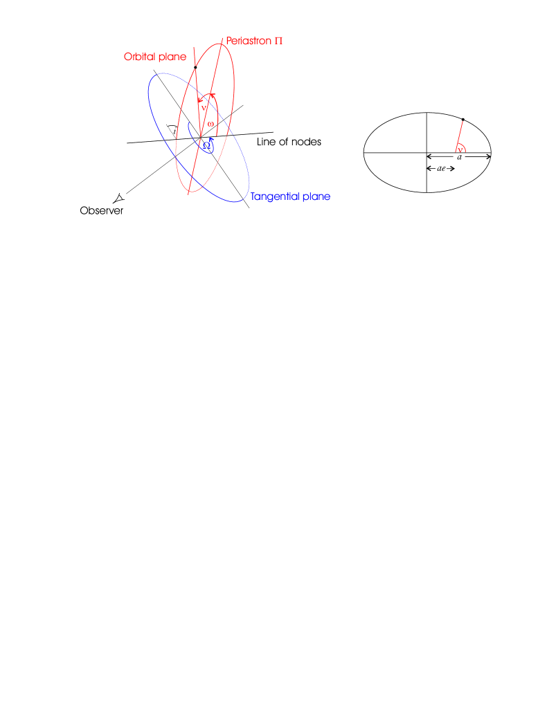
Figure 1.1: Definition of the orbital elements.

The dynamical elements characterizing the size and shape of the orbital ellipse are the semi-major axis $a$, the eccentricity $e$ and the period $P$. Often the time of periastron $T_{p}$ is also used to specify the timing of the orbit.
The position of the orbit in space with respect to the local coordinate system is characterized by three solid angles. The intersection of the orbital plane with the plane perpendicular to our line of sight is called the line of nodes. It connects the two points where the orbit intersects the tangential plane. These points are called ascending node and descending node, depending on whether the companion passes the tangential plane from South to North or North to South, respectively. The angle from the coordinate zero point of the reference plane, the projection of the North celestial pole, to the ascending node is the longitude of the ascending node $\Omega$. It is measured Eastward.
The angle between the reference plane and the orbital plane is called the inclination $i$. If the orbit of the companion is direct, i.e. the position angle increases with time, then $i<90\hbox{${}^{\circ}$}$, in the case of an retrograde orbit $90\hbox{${}^{\circ}$}<i<180\hbox{${}^{\circ}$}$. For an inclination of $0\hbox{${}^{\circ}$}$ or $180\hbox{${}^{\circ}$}$ the orbit is seen face-on, for $i=90\hbox{${}^{\circ}$}$ the orbit is seen edge-on.
The third angle is the longitude of periastron $\omega$. It specifies the orientation of the orbit in the orbital plane and defines the angle of the direction to the periastron $\Pi$ from the line of nodes.

1.2 Detection Methods

1.2.1 Pulsar Timing

By surprise the first planetary-mass objects detected were orbiting a pulsar and had masses close to the terrestrial mass. Two planetary objects with $2.8\leavevmode\nobreak\ M\hbox{${}_{\oplus}$}$ and $3.4\leavevmode\nobreak\ M\hbox{${}_{\oplus}$}$ with 98.88 days and 66.54 days period, respectively, were found to orbit the millisecond pulsar PSR B1257 + 12 (Wolszczan, 1994; Wolszczan and Frail, 1992). Later also a third component was found in this system. Pulsars are extremely rapidly rotating neutron stars which emit mostly radio emission in a very narrow light-cone. If the alignment with the observer is favorable, a pulse effect can be observed similar to a lighthouse. These pulses are very precise and stable in time, which makes it possible to detect small variations in the periodicity. Such a variation can occur when a companion is orbiting the pulsar, causing a positional shift of the pulsar around the barycenter of the pulsar-companion system. The motion of the pulsar around the barycenter leads to a change in light travel time of the incoming pulses, which becomes manifest in a delay or early arrival of the pulse signals $\tau$.

$$\tau=\sin{i}\left(\frac{a_{p}}{c}\right)\left(\frac{m_{p}}{M_{*}}\right)$$ (1.1)

Here $a_{p}$ is the semi-major axis of the planet’s orbit, i the inclination of the orbit, $M_{p}$ the planetary and $M_{*}$ the pulsar mass and $c$ stands for the speed of light. With this method one can measure the period of the planet, its eccentricity and the projected planet to star mass ratio. Because of the projection of the true motion of the pulsar onto the radial direction between the observer and the pulsar, one only measures a minimum mass for the companion which is still dependent on the inclination of the orbital plane, assuming a known mass for the pulsar.

1.2.2 Radial Velocity Measurements

The most successful detection method so far has been the radial velocity (RV) method. The first extrasolar planet around a solar type star was discovered this way by Michel Mayor and Didier Queloz (Mayor and Queloz, 1995). The radial velocity method measures, as the pulsar timing method, the movement of the star due to an unseen planet in the direction of the line of sight. In this process the Doppler-shift of the spectral lines is measured. High precision spectral line measurements can be performed by comparing the stellar spectrum with a set of reference lines. This reference lines are superimposed on the stellar spectrum and can be produced for example by an iodine cell in the light path of the spectrograph. If the target star has a planet, it will exhibit a Doppler shift $\Delta\lambda/\lambda=v/c$, with the same period as the planetary orbit. The spectral lines will move redward when the star is moving away from the observer and bluewards when it is approaching. These variations only measure the component of the motion projected onto the line of sight of the observer and hence only a minimum mass, $m_{p}\sin{i}$ of the planet orbiting the star can be measured. The semi-amplitude of the radial velocity variation is given by:

$$K=\left(\frac{2\pi G}{P}\right)^{1/3}\leavevmode\nobreak\ \frac{m_{p}\sin{i}}{(M_{*}+m_{p})^{2/3}}\frac{1}{\sqrt{1-e^{2}}}$$ (1.2)

where $P$ is the planetary orbital period, $e$ the eccentricity and $G$ the gravitational constant. $K,P$ and $e$ can be derived from the shape of the Doppler curve. Also the argument of periastron, $\omega$, and the time of periastron, $T_{p}$, can be derived from the RV curve. Estimating the stellar mass $M_{*}$ from stellar models and assuming $m_{p}\ll M_{*}$ one can determine $m_{p}\sin{i}$. With Kepler’s third law $P[\rm yr]=(a_{p}[\rm AU])^{3/2}(M_{*}/M\hbox{${}_{\odot}$})$, where $M\hbox{${}_{\odot}$}$ is one solar mass, one can also derive the semi-major axis $a_{p}$ of the planet.
If the mass of the companion cannot be neglected, one cannot derive $m_{p}\sin{i}$ but has to use the mass function for the star-planet system instead:

$$f(m)=\frac{(m_{p}\sin{i})^{3}}{(M_{*}+m_{p})^{2}}=\frac{PK^{3}(1-e^{2})^{3/2}}{2\pi G}$$ (1.3)

and a minimum semi-major axis of the stellar wobble:

$$a_{*}\sin{i}=K\cdot P\frac{\sqrt{1-e^{2}}}{2\pi}$$ (1.4)

The fact that the RV measurements only yield the component of the orbital motion in the direction of the observer’s line of sight, can lead to the case that a low-mass star orbiting another star with a small inclination of the orbit is interpreted as the signal produced by a planetary companion orbiting at a high inclination. However, this is very unlikely if one assumes random orientation of the orbits. The most likely observable inclination would be close to edge-on, with a median inclination of $60\hbox{${}^{\circ}$}$ (Kürster et al., 1999).

The RV technique has the advantage of being mostly independent of the distance. The only distance related limitation is that the more distant the stars are the fainter they are, leading to a lower signal to noise ratio in the spectra. The precision possible for the RV detection method is about 1 m/s, limited by intrinsic stellar turbulence and activity in even the most stable stars. Because of this, spectral types of F, G, and K are preferred for this technique, as later type stars are often too faint for adequate signal to noise and early type stars have much less spectral lines to measure and are limited in the line positioning accuracy due to the spectral line broadening. The RV measurements are strongly biased towards close-in orbits and high masses, as the RV semi-amplitude $K$ is higher for shorter periods $P$, i.e. smaller separations from the host star and higher masses of the companion, explaining the high number of Hot-Jupiter detections.

For this reason most of the large radial velocity surveys target non-active main sequence stars (e.g. Tinney et al., 2001; Queloz et al., 2000), but also M-stars (e.g. Kürster et al., 2006; Zechmeister et al., 2009; Bonfils et al., 2004) and young stars (Setiawan et al., 2008) are being monitored. Low mass planets are thought to be found more easily around M-stars, as their stellar mass is smaller and the effect of perturbations of smaller planets is easier to detect, but on the other hand M-stars are fainter and therefore the precision obtained in the RV measurements is not as high as for solar-type stars.

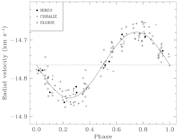
Figure 1.2: Radial velocity curve of the system HD 209458 (see Mazeh et al., 2000). The planetary companion has a mass of $0.685\leavevmode\nobreak\ M_{J}$ and orbits its parent star in 3.525 days. The different symbols show the data taken with the different instruments and the solid line is the best fit Keplerian orbit.

1.2.3 Transits

If a planet passes between its host star’s disk and the observer, the observed flux drops by a small amount. The amount of the dimming depends on the relative sizes of the planet and star and its maximum depth is given by $R_{p}/R_{*}^{2}$, where $R_{p}$ is the radius of the planet and $R_{*}$ that of the star. So, if one can estimate $R_{*}$, one has a direct measure for the radius of the planet, something one can only measure with this method. From the periodicity of the transit event one gets the orbital period $P$ and if one can estimate the stellar mass $M_{*}$ one can derive the semi major axis of the planetary orbit from Kepler’s third law. The shape of the dip in the light curve depends on the inclination of the system, which has to be close to $90\hbox{${}^{\circ}$}$ to observe a transit. Due to simple geometric reasons, this is the case only for a small minority of planets. Additionally the probability of a transit is proportional to the ratio of the diameter of the star and the diameter of the orbit. The longer the orbital period, the smaller is the chance of a proper alignment. Also the chance of seeing the transit by measuring at the right time is decreasing with longer orbital periods. Nevertheless around 70 planets have already been detected using this method with likely more to come from the ongoing surveys of the KEPLER (e.g. Basri et al., 2005; Borucki et al., 2010) and CoRoT (e.g. Deleuil et al., 2010; Bordé et al., 2003) missions, which observe large areas on the sky with thousands of stars.
The transit method for detecting exoplanets is also biased to close-in orbits, as is the radial velocity method. If one can combine the two methods and solve the degeneracy of the orbital inclination, one can compute the true mass of the planet, and, together with the radius determined from the transit, the density of the planet.

Figure 1.3: Transit light curves for the planetary system HD 209458. Left the first measurements from ground (Charbonneau et al., 2000) with the STARE Project Schmidt camera and right a light curve obtained with the STIS instrument aboard the Hubble Space Telescope (Brown et al., 2001). The solid lines show the transit shape for the best fit model and the dashed lines in the left panel show additionally the transit curves for a planet with a 10% larger and smaller radius than the one from the best fit, respectively.

Comparing observations of spectra of the star during transit and outside of transit can yield spectral features of the transmission spectrum of the planetary atmosphere if the signal to noise ratio of the spectra is high enough. Such observations were conducted for the first transiting planet detected, HD 209458 (Charbonneau et al., 2000, 2002).

Likewise one can use this so-called secondary eclipse, when the planet is behind the star, to measure the thermal flux emitted from the planet. Hot Jupiters typically have a thermal flux which is ’only’ about $10^{-4}$ times smaller than that of the star, which makes it possible to indirectly measure it. When the planet is behind the star, one has the unique opportunity to measure the true brightness of the star. Subtracting this from the combined planet + star brightness one can derive the thermal flux, $F_{p}$ of the planet assuming a known distance of the system. Under the assumption of blackbody radiation $F_{p}$, is given by:

$$F_{p}=4\pi R^{2}_{p}\sigma T^{4}_{p}$$ (1.5)

where $\sigma$ is the Stefan-Boltzmann constant and $T_{p}$ the effective temperature of the planet. Deducing $R_{p}$ from the depth of the transit light curve, one can infer the effective temperature of the planet.
Comparing the spectrum of the star + planet with the one of the star observed during secondary eclipse, provides the opportunity to carry out infrared spectroscopy of the planet. The space telescope Spitzer has been used mainly for this purpose and the upcoming James Webb Space Telescope (JWST) will provide even more progress in this field. But also from the ground first approaches have started to examine the secondary eclipse and its measurands (Swain et al., 2010).

1.2.4 Gravitational Microlensing

Due to general relativistic effects a light path is bent in the presence of a gravitational field. In principle any massive object can act as a lens, bending the light of a background object and causing a temporary magnification of the brightness of the background object. Such lensing can be observed on a galactic scale, where for example a massive cluster in the foreground is acting as a lens for distant galaxies. In the case of a perfect alignment the lens would cause the background object to appear as a ring, the so-called Einstein-Ring, with an angular radius of:

$$\theta_{E}=\sqrt{\frac{4GM_{*}(D_{S}-D_{L})}{c^{2}D_{L}D_{S}}}$$ (1.6)

where $D_{L}$ is the distance to the lens, $D_{S}$ the distance to the background source and $M_{*}$ the mass of the lens. In the case of an imperfect alignment several single images of the background object are imaged around the lens.

In the case relevant for planetary detection with the gravitational lensing method, a star with a planetary companion acts as the lens and the background object is a distant star. The probability of an alignment among two stars is very small, but increases towards the galactic center. But even there it is only about one in $10^{6}$. Contrary to the lensing on a galactic scale it is not possible with current instrumentation to resolve the Einstein ring on the stellar scale. Instead one measures the total magnification which depends on the angular separation between the lens and the background object $u$ and its change with time. The magnification factor $Q$ of the event is given by:

$$Q(t)=\frac{u^{2}(t)+2}{u(t)\sqrt{u^{2}(t)+4}}$$ (1.7)

As the lens passes the background star, $Q$ changes with time, and measuring the light curve in a close enough time sample during the event yields information about the lensing star. If a planet is in orbit around the lensing star and the already magnified image of the background star comes close to this planet, then the planet’s own gravitational potential, distorting the star’s potential, becomes also a visible effect. An additional brightening will occur on top of the brightening due to the lensing star, causing a sharp peak in the light curve, see Fig. 1.4. This detection method is sensitive down to very low-mass planets and also to planets orbiting very distant stars.

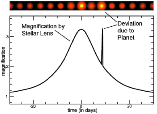
Figure 1.4: Light curve of a gravitational lensing event of a star with a planet. On top the brightening due to the lensing of the star and later the planet is shown. Image taken from the Microlensing Planet Search Project homepage.

As these events do not repeat and two stars need to be aligned, this approach is challenging. The current approach is to monitor a large number of planets and alert other collaborating observatories and institutes as soon as a lensing event is detected, which then also observe the event if possible. This provides a good time sampling of the light curve. A very successful survey is the OGLE survey (Optical Gravitational Lensing Experiment), which has detected several planets to date (see e.g. Udalski et al., 1993).

1.2.5 Direct Imaging

Direct imaging of an exoplanet yields a wide range of information about the planet. One can characterize it spectroscopically, providing information about the atmosphere and measure its astrometric motion to derive information about the orbit. But to directly image a planet next to a bright star is a challenging task, given the brightness contrast and the small angular separation typical for exoplanetary systems. Jupiter for example would only have a 4 arcsecond separation from the sun when viewed from Alpha Centauri and typical angular distances of known exoplanets are much smaller.

Exoplanets are cool objects with temperatures in the range of a few 100 K, which makes their thermal brightness in the visual negligible. The light observable from the planet in this wavelength range is reflected light from the primary star. For an Earth-like planet the flux ratio between planet and star is $\sim 10^{-10}$. This is an almost impossible high contrast for today’s instruments, given the very small separation between the star and the planet of $0.1-1\hbox{${}^{\prime\prime}$}$ for nearby stars, and additional techniques have to be used. One possibility to nevertheless image the planet is coronography, where most of the light from the star is blocked, so the planetary signal becomes visible. Other methods include spectral differential imaging, the system is imaged simultaneously in two different filters and the two images are subtracted afterwards, angular differential imaging, the system is imaged with two different position angles and the two images are subtracted afterwards, and nulling interferometry, see below.
In the infrared wavelength regime, the thermal emission of the planets is higher and peaks in the mid-infrared. The younger and hotter a planet is, the higher is its IR flux. For an Earth-like planet the star-planet flux ratio goes down to about $10^{-7}$. But at the same time, the spatial resolution is getting worse with longer wavelengths. Using interferometry is one solution, as it is easier at longer wavelengths and improves the spatial resolution in addition to the lower flux contrast. Supplementary nulling interferometry is possible. The light from two telescopes is brought together with a shift of $\lambda/2$ in one light path, so the two beams interfere destructively on-axis where the star is centered. In the ideal case, this cancels out all light at zero phase, but keeping the flux at other phases and hence is working like a coronograph.

Most of the extrasolar planets detected with direct imaging so far have bigger separations from their host stars than the ones detected with radial velocity or transits. But with the already installed and near future instruments for direct imaging with adaptive optics correction and coronography and/or interferometry more and more planets will be detected closer to their stars.
One of the first extrasolar planetary systems whose orbital motions were confirmed via direct imaging is the system HR 8799. HR 8799 is a young ($\sim 60$ million year old) main sequence star located 39 parsecs away from the Earth in the constellation of Pegasus. The system contains three detected massive planets and also a debris disk. The planets were detected by Christian Marois with the Keck and Gemini telescopes on Mauna Kea, Hawaii (Marois et al., 2008). Just recently the first spectrum of an exoplanet was obtained from the middle one of the three planets orbiting HR 8799 with the NACO instrument at the VLT (Janson et al., 2010). This is the first step into a new and amazing area of extrasolar planet characterization. In Fig. 1.5 the direct image of the three exoplanets is shown.

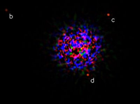
Figure 1.5: Image of the three planetary companions to the star HR 8799 produced by combining J-, H-, and Ks-band images obtained at the Keck telescope in July (H) and September (J and Ks) 2008 (Marois et al., 2008). The three planets b, c, d have masses around 7, 10 and $10\leavevmode\nobreak\ M_{J}$ respectively, inferred from photometry and fitting evolutionary tracks.

1.2.6 Astrometry

Astrometry is the oldest measurement technique in astronomy. The method consists of precise measurements of the position of a star on the tangent plane on the sky relative to a reference frame and has been used for centuries to measure proper motions, parallaxes and astrometric orbits of visual binaries. The gravitational influence of an orbiting planet causes the star to move around their common center of mass in a small, down-scaled orbital movement. Assuming $M_{*}\gg m_{p}$ a combination of the law of the lever for the two-body problem with Kepler’s $3^{rd}$ law gives the semi-amplitude $a_{*}$ of the stellar wobble due to the companion in radians:

$$a_{*}=\frac{m_{p}}{r}\leavevmode\nobreak\ \left(\frac{G}{4\pi^{2}}\right)^{1/3}\leavevmode\nobreak\ \left(\frac{P}{M_{*}}\right)^{2/3}$$ (1.8)

Here $r$ is the distance of the system, $M_{*}$ is the stellar mass , $m_{p}$ the companion’s mass, $P$ the orbital Period and $G$ the gravitational constant. The astrometric signal becomes stronger the more massive the companion, and/or the less massive the primary and the bigger the separation between the two components. This makes this detection method complementary to RV and transit detection, which are most sensitive to close-in planets. As one can see from Equ. 1.8, the astrometric detection of a planetary companion is very sensitive to the distance of the system, which limits this technique to applications to nearby stars. The astrometric signals for some of our own solar systems planets seen from 10 pc distance and examples for a hot Jupiter and an Earth-like planet orbiting a solar-type star, as well as several other examples are listed in Tab. 1.1. The values are calculated for the case the full major axis $a_{*}$ is measured and are given as the peak-to-peak astrometric signal, $\alpha=2*a_{*}$. If the orientation of the system is such, that not the full major axis is measurable, the astrometric signal is even smaller. No matter how the system is oriented, one can always measure at least the signal of the minor axis.

Planet	$a_{p}$ [AU]	$\alpha$		Primary mass
Jupiter ♃	5	0.96	mas	$1\leavevmode\nobreak\ M\hbox{${}_{\odot}$}$ (sun-like star)
Jupiter ♃	1	0.19	mas	$1\leavevmode\nobreak\ M\hbox{${}_{\odot}$}$
hot Jupiter	0.05	9.5	$\mu\rm as$	$1\leavevmode\nobreak\ M\hbox{${}_{\odot}$}$
Neptune ♆	1	1.3	$\mu\rm as$	$1\leavevmode\nobreak\ M\hbox{${}_{\odot}$}$
Neptune ♆	30	0.31	mas	$1\leavevmode\nobreak\ M\hbox{${}_{\odot}$}$
Earth ♁	1	0.60	$\mu\rm as$	$1\leavevmode\nobreak\ M\hbox{${}_{\odot}$}$
Brown dwarf ($30\leavevmode\nobreak\ M_{J}$)	0.5	2.9	mas	$1\leavevmode\nobreak\ M\hbox{${}_{\odot}$}$
Brown dwarf ($30\leavevmode\nobreak\ M_{J}$)	30	171.9	mas	$1\leavevmode\nobreak\ M\hbox{${}_{\odot}$}$
Brown dwarf ($30\leavevmode\nobreak\ M_{J}$)	1	11.5	mas	$0.5\leavevmode\nobreak\ M\hbox{${}_{\odot}$}$ (M Dwarf)
Brown dwarf ($30\leavevmode\nobreak\ M_{J}$)	15	171.9	mas	$0.5\leavevmode\nobreak\ M\hbox{${}_{\odot}$}$
Jupiter ♃	1	0.38	mas	$0.5\leavevmode\nobreak\ M\hbox{${}_{\odot}$}$
Jupiter ♃	15	5.7	mas	$0.5\leavevmode\nobreak\ M\hbox{${}_{\odot}$}$
Earth ♁	1	1.2	$\mu\rm as$	$0.5\leavevmode\nobreak\ M\hbox{${}_{\odot}$}$
Earth ♁	0.1	0.12	$\mu\rm as$	$0.5\leavevmode\nobreak\ M\hbox{${}_{\odot}$}$

Table 1.1: Examples for astrometric signals for planets with different masses and semi major axes, orbiting a sun-like star or a dwarf star with $0.5\leavevmode\nobreak\ M\hbox{${}_{\odot}$}$. All values are calculated for a distance of 10 pc and the case that the full major axis is measured.

If one has obtained astrometric data points which cover a sufficient part of the orbit, all orbital parameters can be determined. Especially with a known distance and stellar mass, the true mass of the companion can be calculated. Astrometric planet detection gives therefore more information about the detected companion than RV does. But to derive the orbital motion of the star due to the companion, one has to disentangle this motion from proper motion of the star and the parallactic movement of the Earth bound observer and the orbital motion. Astrometric position determination always needs a reference system to which the position of the target star is referenced. Preferable would be a fixed system, but this is rather difficult to set up and sometimes not possible. To a much higher precision, positions can be determined relative to another system. For planet detection this can be a star asterism in the same field of view (FoV) as the targeted star. Since the stars used to set up the reference frame have their own proper motion and parallactic movement, the proper motion and parallax of the target star can only be derived relative to this reference frame and do not need to be the same as the absolute ones. If one is only interested in the orbital movement due to a companion, one does not need to know the absolute proper motion and parallax, but of course, it is always beneficial to know the absolute parameters, e.g. to calculate the distance of the target.

Astrometric measurements have been used to determine astrometric binary systems for quite a long time. One of the first comments about the detection of an unseen companion was made by William Herschel in the late 18th century, when he claimed an unseen companion being responsible for the position variations of the star 70 Ophiuchi. Other systems were announced in the coming two centuries, but all of them were later vitiated or are still under discussion.
The only measurements of an astrometric signal due to an unseen companion were obtained with the Hubble Space Telescope (HST). In 2002 Benedict et al. succeeded in detecting the astrometric motion of the previously with RV discovered planet around the star Gliese 876, and in 2006 the signal of the planet orbiting $\epsilon$ Eridani (Benedict et al., 2006) (see also Bean et al., 2007; Martioli et al., 2010; Benedict et al., 2010, for more examples).
In 2009 a planet orbiting the ultracool dwarf VB 10 (= GJ 752B), spectral class M8 V, was discovered from ground with astrometry using the wide-field seeing limited imager at the Palomar 200-inch telescope within the Stellar Planet Survey program (STEPS) (Pravdo and Shaklan, 2009). The reflex motion of VB 10 around the system barycenter compared to a grid of reference stars in the same FoV was monitored over 9 years. The best fit Keplerian orbit yields a $6.4^{+2.5}_{-3.1}\rm\leavevmode\nobreak\ M_{J}$ planet in an 0.74 year almost edge-on orbit ($i=96.9\hbox{${}^{\circ}$}$). Unfortunately, lately obtained RV observations with the high precision spectrograph HARPS at the ESO 3.6 m telescope in La Silla, Chile, were not able to confirm this planet, but instead ruled out the astrometric orbit solution (Bean et al., 2010).

Figure 1.6: Left: Astrometric motion of the Sun’s center around the barycenter of the solar system due to all planets over 50 years, viewed face-on from a distance of 30 light years (Jones, 2008). The dashed circular line shows the motion of the Sun due to only Jupiter. The size of the disk of the sun is shown in the upper right corner for comparison. Right: Astrometric orbit of HD 33636, a G0 V star at 28.7 pc distance (Bean et al., 2007). Open circles are the HST position for each epoch connected with a line to the positions calculated by the fit model. The open square shows the predicted position of periastron passage.

Measuring an astrometric signal from ground is very difficult, as the changes of the stellar position are very small and the atmospheric and systematic distortions, such as plate-scale variations between different observations, may be larger. The usage of a correction of the atmospheric distortions with adaptive optics and determining the plate-solution with great care, as done in the context of this work, can reduce these difficulties and enable one to go down to the desired $\sim 1$ mas precision needed to detect and characterize companions in wider orbits. However, to detect Earth-like planets orbiting solar-like stars, one needs a higher precision in the astrometric measurements. Interferometry makes it possible to achieve precisions about a few microarcseconds. The already installed and soon available instrument PRIMA at the VLT will boost the number of planets detected with astrometry. The spacebound astrometric mission GAIA, planned launch in August 2011, will also make a huge contribution in stellar position measurements and with this yield a huge number of newly detected Jupiter-size planets (Sozzetti et al., 2001). Special designed missions, such as SIM PlanetQuest (e.g. Catanzarite et al., 2006; Unwin et al., 2008), which are specialized for astrometric measurements both for parallax movements and exoplanet detections around stars in the solar neighborhood, will reach accuracies about one microarcsecond and will be sensitive down to Earth-like masses. But also the astrometry obtained from the photometric transit mission KEPLER may be used for astrometric planet detection, given its stable and precise pointing.

Combination of Radial Velocity Data and Astrometric Data

Planet detections with radial velocities only yield a minimum mass for the companion as one cannot determine the inclination of the orbital plane with respect to the observer. The measured semi-amplitude of the velocity change is the projection of the true motion onto the line of sight from the observer to the star. Companions detected with radial velocities should therefore be seen as exoplanet candidates for the time being.
Astrometry yields the whole parameter set necessary to describe the full orbital motion in space, but typically a large number of high precision measurements need to be obtained. The complete astrometric fit for the motion of a star with a companion in space includes:
$\alpha_{0},\delta_{0}$ two coordinate zero points $\mu_{\alpha},\mu_{\delta}$ proper motion in right ascension and declination $\pi$ parallax $a_{*}$ semi-major axis of the orbit $e$ eccentricity $P$ orbital period $\omega$ longitude of periastron $\Omega$ longitude of the ascending node $i$ inclination

To solve for these 11 parameters one has to obtain at least 11 epochs of measurement, preferentially more for reasons of robustness of the fit and taken the present noise in the data into account.

Combining radial velocity and astrometric measurements yields the whole three dimensional orbit as one combines measurements which are sensitive to the movement in the direction of the line of sight and in the plane perpendicular to it. Taking the orbital parameters inferred from radial velocities, $P,e,\omega,a$, one is left with only seven parameters to solve for with the astrometric fit. If one additionally can infer the proper motion and parallax independently, only the inclination and longitude of the ascending node, as well as the coordinate zero points, need to be determined. However, most of the time this is not possible, as either the precision of these parameters is not sufficient, or one has to determine the proper motion and parallax relative to the local reference frame. Combination of the two measurement techniques has advantages and disadvantages. The advantage of this approach is that normally the radial velocity measurements are obtained with much higher precision than what is possible for the astrometric measurements. One can therefore hold the parameters from the RV fit fixed. A disadvantage or rather a constraint is the circumstance that RV detections are most sensitive to close-in companions and astrometry to companions in wider orbits. Therefore the astrometric signal for most of the planets detected by radial velocities are very small and difficult to detect. But with the upcoming specialized astrometric instruments, these will come more and more into range.

The astrometric measurements of radial velocity exoplanet candidates conducted with the HST Fine Guidance Sensor, pushed three out of five candidates from the planetary regime into the brown dwarf or low mass star regime:

Planet cand.	$M\sin{i}[M_{J}]$	$M[M_{J}]$	inclination	Reference
HD 33636 b	9.3	$142\pm 11$	$4.1\hbox{${}^{\circ}$}\pm 0.1\hbox{${}^{\circ}$}$	Bean et al.,2007
		M dwarf star
HD 136118 b	12	$42^{+11}_{-18}$	$163.1\hbox{${}^{\circ}$}\pm 3.0\hbox{${}^{\circ}$}$	Martioli et al.,2010
		Brown Dwarf
HD 38529 c	13.1	$17.6^{+1.5}_{-1.2}$	$48.3\hbox{${}^{\circ}$}\pm 0.4\hbox{${}^{\circ}$}$	Benedict et al.,2010
		Brown Dwarf

This shows how important it is to obtain complementary measurements to solve for the whole 3D orbit and calculate the true mass of the exoplanet candidates.

Combination of radial velocity data with astrometry provided by the HIPPARCOS satellite has also been done (Perryman et al., 1996; Mazeh et al., 1999; Zucker and Mazeh, 2000). Han et al. (2001) used the HIPPARCOS intermediate astrometric data to fit the astrometric signal of stars known to have a possible planetary companion found by radial velocity. Most of the expected astrometric perturbations were close to or lower than the precision obtained from the HIPPARCOS data. The conclusion of this statistical study was that a significant fraction of the exoplanetary systems are seen edge-on, which would push their masses to also significantly higher masses. Pourbaix (2001) later showed that the high inclinations found by Han et al. are artifacts of their adopted fitting procedure. As the reason for that he named the size of the orbit with respect to the precision of the astrometric measurements, meaning, the ’measured’ astrometric signal was not large enough compared the astrometric precision. Future astrometric missions, such as GAIA will lead to much higher precisions in the astrometric measurements, thus leading to better constraints on the orbital inclination.

1.3 Brown Dwarfs

In the same year, at the same conference, the first widely accepted brown dwarf (BD), Gliese 229B (Nakajima et al., 1995), and the first extrasolar gas giant planet, 51 Peg b (Mayor and Queloz, 1995), were announced to the astronomical community. Now there are around 720 BDs known to exist as companions to nearby stars, in young clusters and most frequently as faint isolated systems within a few hundred parsecs in the solar neighborhood. Brown dwarfs are star-like objects with a maximum mass between 0.07 and 0.08 M_⊙, depending on their metallicity. This mass limit for BDs is defined by the disability to sustain stable hydrogen fusion reactions in their cores and sets a division between stars and brown dwarfs. But BDs are massive enough to be able to burn deuterium in their cores at the beginning of their evolution, followed by a steady decline in their luminosity and effective temperature with time, once their supply of deuterium is exhausted.
The division between brown dwarfs and giant planets is yet not clear and still under debate. Two possible ways of defining brown dwarfs and giant planets are under discussion. One widely used definition is based on the mass limit to burn deuterium, which would define an object with less than $13\rm\leavevmode\nobreak\ M_{\rm Jup}$ as a planet (Saumon et al., 1996; Chabrier et al., 2000). This is also the IAU definition for brown dwarfs, which considers objects above the deuterium burning mass limit as brown dwarfs. The definition can be applied to both companions and isolated objects and is the reason why very-low mass objects in clusters are sometimes called free-floating planets. A drawback of the definition of the border between BDs and giant planets over the deuterium burning limit is that unlike the hydrogen burning limit, the ability to fuse deuterium is insignificant for the physical properties of BDs and therefore describes no meaningful boundary for the evolution of low mass objects (Chabrier et al., 2007). In fact there are more differences in stellar structure and evolution between high and low mass stars than for low mass brown dwarfs and giant planets. Also the mass determination with evolutionary models based on the luminosity of the objects is often uncertain, so a definitive conclusion whether an object is above or below the deuterium burning mass limit is difficult. For example the best mass estimate for the object GQ Lup b is $10-40\rm\leavevmode\nobreak\ M_{\rm Jup}$ (McElwain et al., 2007; Seifahrt et al., 2007), hence both definitions, planet and brown dwarf, are possible. Determining the mass dynamically and therefore independent of the models puts more constraints on the evolutionary theories for these low mass objects and help to better understand their mass distribution and formation processes, but this is only measurable for brown dwarfs which are bound in a system.
The other definition to distinguish brown dwarfs and giant planets is based on their formation processes. Here a planet is a substellar object formed in a circumstellar disk and a brown dwarf formed through cloud fragmentation like a star. This definition also has its drawbacks, as it is obviously difficult to tell the formation process of a given substellar object. It is for example most likely for wide massive companions to be formed by cloud fragmentation rather than in a stellar disk, but for lower mass companions in intermediate orbits ($8\rm\leavevmode\nobreak\ M_{\rm Jup},@\leavevmode\nobreak\ 20\rm\leavevmode\nobreak\ AU$) it will be more difficult to determine the formation mechanism (Luhman, 2008). So neither of the definitions provides a clear distinction between brown dwarfs and giant planets. The most commonly accepted one at the moment is the one of the IAU, that distinguishes substellar objects by their mass. Independent of their formation process, objects below $13\rm\leavevmode\nobreak\ M_{\rm Jup}$ which orbit a star or stellar remnant are planets and objects with masses above this deuterium burning mass limit and below the hydrogen burning limit ($13\rm\leavevmode\nobreak\ M_{\rm Jup}-\sim 80\rm\leavevmode\nobreak\ M_{\rm Jup}$) are defined as brown dwarfs.

1.3.1 Brown Dwarf Formation Processes

Similar to the difficulty to define a distinctive boundary between brown dwarfs and giant planets, it is challenging to put constraints on the formation process of brown dwarfs. Several scenarios are under discussion, but none of them can explain all of the available observations. A star-like formation by direct collapse and fragmentation of a molecular cloud, a scaled version of the Jeans model, is one possibility for BD formation (Bate and Bonnell, 2005). Another possibility is the ejection of protostellar embryos that form in a cluster environment, but are ejected due to dynamical interactions before they can accrete enough material to become a star (Reipurth and Clarke, 2001; Umbreit et al., 2005). This scenario has difficulties to explain young wide BD binaries, because these should be ripped off during the ejection, likewise large disks should not survive an ejection, but are nevertheless observed (e.g. Scholz et al., 2006). Photoevaporation of their accretion envelope by the radiation of a nearby massive and hot star (Whitworth and Zinnecker, 2004), as well as instabilities in massive disks, followed by a pulling off of the still substellar companions through dynamical encounters with other stars can produce isolated free-floating brown dwarfs (Goodwin and Whitworth, 2007; Stamatellos and Whitworth, 2009). Turbulence in a molecular cloud can produce local over-densities that can collapse and form a compact low mass object. This turbulent fragmentation could explain the formed brown dwarfs as the low-mass tail of the regular star formation process. Also the continuity in disk fraction, the ratio of stars or BDs without a disk to those having a disk, from the stellar to the BD regime (Caballero et al., 2007) favors this formation scenario. None of these scenarios can be seen as the dominant contributor to the brown dwarf population, neither one can explain all observations. Most likely the formation processes of brown dwarfs depend on the stellar environment and its varying initial conditions from case to case, leading to a changing relevance of the individual scenarios.

1.3.2 The Brown Dwarf Desert

Radial velocity surveys to find substellar companions orbiting their host stars have led to the detection of a variety of exoplanets and brown dwarfs. They also led to the definition of the “brown dwarf desert”, the absence of BD companions relative to giant planets and stellar companions to low-mass stars at separations less than 3 AU (Marcy and Butler, 2000). The BD companion frequency at separations > 1000 AU is at least 10 times higher than that of separations of only a few AU, which is $\approx 0.5\leavevmode\nobreak\ \%$ (Gizis et al., 2001; Neuhäuser and Guenther, 2004). The frequency of stellar companions at small separations is $13\pm\leavevmode\nobreak\ 3\%$ (Duquennoy and Mayor, 1991; Mazeh et al., 1992), at least a factor 30 larger than the BD frequency, whereas at larger separations the ratio of frequencies of stellar and substellar companions is between $\sim 3$ and 10 (McCarthy and Zuckerman, 2004). At wider separations to solar-type stars it appears therefore that the brown dwarf desert is no longer present (Luhman et al., 2007). Fig. 1.7 depicts the brown dwarf desert in mass and period. The plot is taken from Grether and Lineweaver (2006) and shows the estimated companion masses versus the period of the companions. The lack of brown dwarf companions in short-period orbits can clearly be seen. For more details about the sample and the companion mass estimates see Grether and Lineweaver (2006).

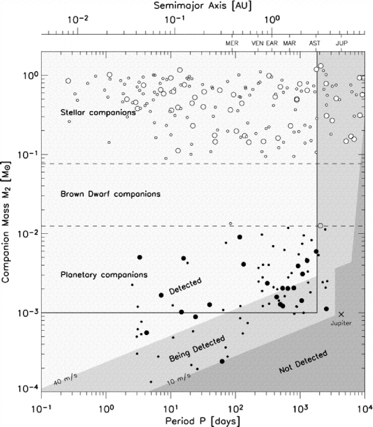
Figure 1.7: Brown dwarf desert in mass and period. Shown are the companion masses $M_{2}$ versus the period of the companions to sun-like stars. The solid rectangle defines companions with periods smaller than 5 years and masses between $1\rm\leavevmode\nobreak\ M_{\rm Jup}$ and $\sim 1\rm\leavevmode\nobreak\ M\hbox{${}_{\odot}$}$. The stellar (open circles), brown dwarfs (blue circles) and planetary (filled circles) companions are separated by the dashed lines at the hydrogen and deuterium burning limit. The brown dwarf desert for companions with orbital periods $P<5$ years can clearly be seen. The detected, being detected and not detected regions of the mass-period space mark the limit to which high-precision radial velocity measurements were able to detect companions at the time of the analysis leading to this plot (Lineweaver and Grether, 2003). For more details about the plot and the sample see Grether and Lineweaver (2006).

The rareness of close-in BD companions is highly significant since the commonly employed RV searches for sub-stellar companions to stars are very sensitive to such objects as the RV semi-amplitude K is higher for shorter periods P, e.g. smaller separations from the host star (see also Equ. 1.2). Because the RV measurements only result in a minimum companion mass and the HIPPARCOS astrometric precision is mostly not sufficient to distinguish BDs from stellar companions, the masses of the few known close-in BD candidates are often uncertain (Pourbaix, 2001; Pourbaix and Arenou, 2001). RV studies of M dwarfs indicate that the BD desert continues also into the early M dwarf population.

1.4 Goal of this Work

Most planets have been discovered by radial velocity measurements. But RV measurements only yield a minimum mass for the companions and are most sensitive to planets in close-in orbits. Transit measurements can yield the true mass of a companion when combined with RV measurements. But they are also most sensitive to close-in planets, as the probability of an occurring transit is higher for those companions.
However, astrometry yields the full set of orbital parameters and therefore the true mass of a companion. It also opens a new parameter space of planets with a longer orbital period.

The goal of this work is to measure the astrometric signal of the wobble of a star due to its unseen companion. Using adaptive optics aided imaging to detect such a signal I want to show the feasibility of this approach for planet and low mass companion detection and characterization. Seeing limited astrometry has mostly a larger field of view than an adaptive optics imager, but the achieved accuracy is most times not high enough to measure the tiny signal of a planet.
To test whether the astrometric signal is measurable, we chose an object known to harbor a candidate brown dwarf companion found by RV measurements (Kürster et al., 2008). When astrometry can be combined with precision RV measurements the number of orbital parameters to be derived from the astrometric data can be strongly reduced (see Sect. 1.2.6). Also the astrometric signal is higher for such an object than for an exoplanet. Additionally, the companion is a very interesting object as it is a brown dwarf desert candidate. Deriving its true mass, confirming it as a BD or pushing it into the low mass star regime, would be a very interesting result.

Chapter 2 Introduction to Adaptive Optics

Stellar wavefronts are assumed to be spherical waves and are treated as plane waves when they reach Earth because of the immense distance of the stars. But turbulences in our atmosphere lead to random deformations of the incoming wave. Telescope optics collect the light and transform it into an image. In the ideal case, without any distortions, the angular resolution of this image is determined by the bending of the light, this is called the diffraction limit case. For circular apertures the angular diameter of the image of a point source is given by:

$$\theta=1.22\frac{\lambda}{D}$$ (2.1)

where $\lambda$ is the observed wavelength and $D$ is the telescope diameter. Such an image of a point source is called Point-Spread-Function (PSF). The intensity distribution of a PSF has the form as shown in Fig. 2.1.

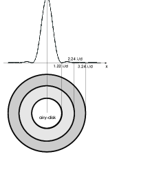
Figure 2.1: The Point-Spread-Function (PSF) of a point source. The diameter of the main maximum is called Airy-disk and has the radius $\theta=1.22\lambda/D$ (from Stumpf (2004)).

The inner part of the distribution is called Airy-disc and it has the radius $1,22\frac{\lambda}{D}$. Two close point sources can only be imaged separately if the maximum of the one PSF falls onto the first minimum of the other PSF.

Due to the atmosphere, part of the intensity contained in the PSF is moved from the maximum to the outer parts of the light distribution. Details are smeared out and cannot be resolved anymore. In Fig. 2.2 the effects of the atmosphere on an image of a close binary star are demonstrated. In the ideal case without any distortions, one obtains a perfect image for each star with a diameter of $2\theta=2,44\lambda/D$ (Fig. 2.2a).

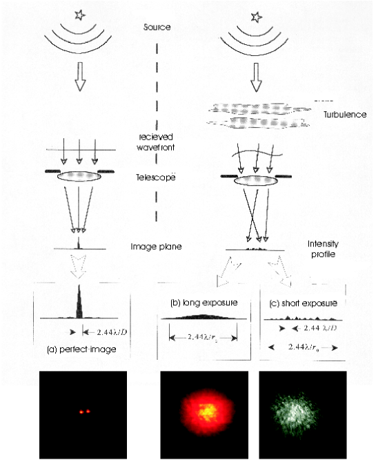
Figure 2.2: Effect of atmospheric turbulence on the image of a close double star (right). Perfect image with no atmosphere (a). Short exposures produce a speckle pattern, which shows a snapshot of the momentary distortions (c). In longer exposures the pattern is smeared out and results in the seeing disk (b). (from Hardy (1998))

If the exposure time is very short, less than 1/50 second, one derives an image consisting of many speckles, which all have a diameter of the diffraction-limited PSF (Fig. 2.2c). This speckle pattern is changing randomly in subsequent images and can be seen as a sketch of the momentary atmospheric distortions. If the exposure time is increased to a multiple of the timescale of the turbulence change in the atmosphere, the speckle pattern is smeared out and one obtains an image of the point source, the so-called seeing disk, with a diameter which is no longer determined by the ratio $\lambda/D$ but by $\lambda/r_{0}$ (Fig. 2.2b). The factor $r_{0}$, called-Fried-Parameter, is an important parameter to describe the atmospheric turbulence. It will be explained in more detail in Chapter 2.1.1. The consequence of the above circumstance is, that even for the bigger but uncompensated telescopes the resolution limit is between 0.5-1 arcseconds or more.
Also the sensitivity of a telescope does not increase in the same way as in the diffraction limit case, which is again due to the atmosphere. Generally, the bigger an aperture, the more light it can collect and the fainter objects it can detect. In the ideal, diffraction limited case the capability of a telescope to detect a point source is $\propto D^{4}$. But this capability is degraded to $\propto D^{2}$ in the seeing limited case, because the image size is no longer determined by the telescope diameter.
There are two possibilities to overcome the image degradations caused by the atmosphere:

• One can go to space and leave the atmosphere behind. Building space based telescopes has the advantage that one can also observe in the wavelength range shorter than $0.3\leavevmode\nobreak\ \mu m$ (UV) where Earth’s atmosphere is opaque, and in the visual and infrared between 0.5 and $2.5\leavevmode\nobreak\ \mu m$ where emission lines from OH-molecules compromise observations. Disadvantages of satellites and space telescopes are their immense costs and technical as well as logistic requirements. The transport into orbit limits their size and weight. They need to be shock-resistent and maintenance or upgrades with new instruments are, if performed at all, expensive and dangerous. But there are certain wavelength ranges which can only be observed from space.

• The other possibility to obtain diffraction-limited images is the usage of an adaptive optics (AO) system. This system consists of two main components, a wavefront sensor, which measures the aberrated wavefront, and a deformable mirror which corrects the wavefronts. Such a system is cheaper to build and to maintain than a space telescope and can be upgraded or modified more easily. In the wavelength range observable from the ground, the ground based telescopes equipped with an AO system are comparable or superior to space based ones, because their primary mirrors can be made considerably larger.
  A more detailed description of an AO system is given in Chap. 2.2.

2.1 Atmospheric Turbulence

The atmosphere is neither static nor homogeneous. Temperature, density and humidity change continuously on different scales of time and space. With it comes a permanent change of the refractive index $n$ of the atmosphere (Clifford, 1978):

$$n(\lambda,P,T)=1+7,76\cdot 10^{-5}\left(1+7,52\cdot 10^{-3}\frac{1}{\lambda^{2}}\right)\frac{P}{T}$$ (2.2)

where $\lambda$ is the wavelength of the light in $\mu m$, $P$ the pressure of the air in $mbar$ and $T$ the temperature of the air in Kelvin. The dependency on the wavelength is small for a broad range of $\lambda$ and the fluctuations of the pressure balance with the speed of sound. But the fluctuations of the temperature are more inertial, and thus dominate the changes of the refractive index. For two parallel light beams which pass through the atmosphere, a difference of the refractive index leads to an adjournment of their relative phases and therefore to a distortion of the previously plane wavefront.
The air masses in different layers of the atmosphere move because of different reasons. In Fig. 2.3 the structure of the atmosphere and a typical turbulence profile is shown.

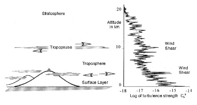
Figure 2.3: Structure of the atmosphere with typical turbulence profile. (Hardy, 1998)

The vertical distribution of the turbulence varies strongly with height (right panel). $C_{n}^{2}$ is a measure for the vertical turbulence strength. On average it is strongest near the ground, the so-called ground layer (GL), because of thermal heating of the ground from sunshine. In the change-over layer between the Troposphere and the Tropopause, at an altitude of around 10 km, the turbulence is dominated by strong winds. A measurement to describe the movement of the air is the Reynolds-number $Re$. It describes whether a flow is laminar or turbulent. $Re$ is given by:

$$Re=\frac{L_{0}\upsilon_{0}}{\eta}$$ (2.3)

Here $L_{0}$ is the characteristic size of a turbulence cell, $\upsilon_{0}$ its characteristic velocity and $\eta$ the kinematic viscosity of the medium, here the air. If the Reynolds-number is smaller than the critical value $10^{3}$, the flow is laminar, otherwise it is turbulent. In air the viscosity is $\eta=15\cdot 10^{-6}m^{2}s^{-1}$ and a typical turbulence cell has a size of $L_{0}=15m$ and a velocity of $\upsilon_{0}=1ms^{-1}$. This yields an average Reynolds-number for the atmosphere of $R_{e}=10^{6}$, which is clearly above the critical value. So the air flow in the atmosphere is mostly turbulent.
To describe and analyze a system as complex as the atmosphere, elaborate models are needed. The most commonly used one in astronomy is the Kolmogorov model (Kolmogorov, 1961). This model describes the turbulence as originating in energy input in large air structures, eddies, with a typical size, the so-called outer scale. This large structures transport the energy loss-free to smaller and smaller structures, the inner scale, till the Reynolds-number is getting smaller than the critical value. The air flow is then laminar and the energy dissipates into thermal heating. Typical sizes of the outer scale are between a few meters at ground level and up to 100 m in the free atmosphere. The inner scale lies between a few millimeters at ground and up to a few centimeters close to the Tropopause.

2.1.1 Fried-Parameter

The Fried-Parameter, also called correlation-length, defines the length over which the mean divergency of the phase-difference to a plane wavefront does not exceed the standard deviation of one radiant (1 rad). It was first introduced and calculated by David L. Fried (Fried, 1965):

$$r_{0}=\left[0.423\left(\frac{2\pi}{\lambda}\right)^{2}\,(\cos\gamma)^{-1}\,\int\limits_{0}^{\infty}C_{n}^{2}(h)dh\right]^{-3/5}$$ (2.4)

$C_{n}^{2}(h)$ is a measure for the vertical strength of the turbulence profile and depends on the height $h$. $\gamma$ is the angle between the line of sight and the zenith. But one can also interpret $r_{0}$ as the size of an aperture that has the same resolution as a diffraction-limited aperture without any turbulence. That means that the resolution of a telescope with a diameter $D$ larger than $r_{0}$, the Full Width at Half Maximum (FWHM), is limited to $FWHM\propto\lambda/r_{0}$ and not anymore $\propto\lambda/D$ as is the case for $D<r_{0}$. The VLT (Very Large Telescope) has a diffraction-limited resolution of $\lambda/D=0.057\hbox{${}^{\prime\prime}$}$ at $\lambda=2.2\mu m$. But the resolution is lowered by the atmosphere to $\lambda/r_{0}\approx 0.7\hbox{${}^{\prime\prime}$}$. One can also see from the equation, that $r_{0}\propto\lambda^{6/5}$, which means the area over which the wavefront error is negligible is growing with wavelength. An $r_{0}$ of typically 10 cm at $0.5\leavevmode\nobreak\ \mu m$ in the visual corresponds to an $r_{0}$ of 360 cm at $10\leavevmode\nobreak\ \mu m$ in the infrared and at $2.2\mu m$ $r_{0}$ is typically 60 cm.

2.1.2 Time Dependent Effects

In the same way as for the spatial case, a time can be defined over which the variance of the wavefront changes account to 1 rad. This time scale is called coherence time $\tau_{0}$. The relation to $r_{0}$ is given over the wind speed $\mathbf{v}$:

$$\tau_{0}=\frac{r_{0}}{|\mathbf{v}|}$$ (2.5)

With an average $r_{0}$ of 60 cm and $\mathbf{v}=10$m/s this yields $\tau_{0}\approx 60$ ms in the infrared at $2.2\mu m$ . To derive a diffraction-limited image, one needs to correct the wavefront errors in this frequency range.
Both $\tau_{0}$ and $r_{0}$ are critical parameters and the larger they are, the more stable the atmosphere is.

2.2 Principles of Adaptive Optics

A powerful technique in overcoming the degrading effects of the atmospheric turbulence is real-time compensation of the deformation of the wavefront by adaptive optics.

2.2.1 General Setup of an AO System

The task of an adaptive optics system is the measurement of the wavefront distortions caused by the atmosphere, the calculation of a correction and its execution. In Fig. 2.4 the principle setup of an AO system is depicted.

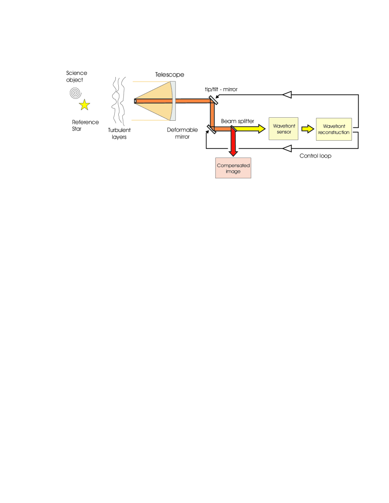
Figure 2.4: Principle setup of an AO system.

The light coming from a star is a plane wavefront (WF) until it is distorted by the Earth’s atmosphere. It passes trough the telescope optics and then reaches the AO system, where it first passes through the correction unit, so that after the first correction only the differential wavefront error between the single measurement cycles has to be corrected. In the ideal case, the wavefront is plane again after the correction. The correction unit often consists of two elements, a tip-tilt mirror that is tiltable in two directions and acts for image stabilization, which is the largest disturbance generated by the turbulence, and a deformable mirror (DM) which is deformed inversely to the incoming WF and compensates for the higher order aberrations.
After the correction unit the light is divided by a beam splitter into two parts. One part, mostly the infrared part of the light, is directly led to the science camera. The other part, mostly the visual light, is led to the wavefront sensor (WFS), which measures the distortions of the WF. If it is necessary to observe and sense in the infrared, for very red objects for example, a intensity-filter is used instead of a dichroic for the beam splitting. With the WF reconstruction unit, wavefront errors are translated into control signals for steering the deformable mirror and the tip/tilt mirror. With sending these steering signals the loop is closed.
Typical frequencies for one cycle of the loop are 1-2 kHz. The frequency depends on the wavelength $\lambda$ in which the observation is conducted, because the time dependent change of the atmospheric disturbance, $\tau_{0}$, is depending on $r_{0}$ and therefore on $\lambda$, see Sec. 2.1. The longer the wavelength, the easier it is to correct the wavefront distortions. Therefore most current AO systems correct for instruments which work in the infrared or even longer wavelengths.

2.2.2 Strehl Ratio

A good way to describe the quality of a partially corrected PSF is the Strehl ratio, which basically corresponds to the amount of light contained in the diffraction-limited core relative to the total flux, (Strehl, 1902). Due to the wavefront distortions, part of the intensity of a PSF (Fig. 2.1) is moved from the peak to the halo. Therefore, the maximum intensity of the PSF is decreased. The Strehl ratio is defined as the ratio between the actual maximum intensity of a point source, $I_{p}$, and the intensity which would be reached by a perfect, diffraction-limited telescope of the same aperture, $I^{*}$. The Strehl ratio can be calculated analytically, if the aberrated wavefront $\Phi(\rho,\theta)$ is known, following (Hardy, 1998):

$$S=\frac{I_{p}}{I^{*}}=\frac{1}{\pi^{2}}\left|\int\limits_{0}^{1}\int\limits_{0}^{2\pi}\exp(ik\Phi(\rho,\theta))\,\rho d\rho\,d\theta\right|^{2}$$ (2.6)

where, $k$ is the wave number and $\rho,\theta$ are polar coordinates. But if the mean quadratic error of the wavefront only amounts up to 2 rad, the Maréchal-Approximation (Maréchal, 1947) is used commonly in astronomy:

$$S\approx\exp^{-\sigma^{2}}$$ (2.7)

Here $\sigma$ stands for the mean-square wavefront error. Typically the Strehl-ratio is less than one percent for a uncorrected system. In case of good conditions and a bright, nearby reference source, the correction is good and the resulting PSF is close to the diffraction limit. A good correction in the K-Band typically corresponds to a Strehl ratio larger than $30\%$.

2.2.3 Anisoplanatism

All adaptive optics systems need a point source to measure the wavefront distortions caused by the atmosphere. Generally this is a suitable reference star, whose wavefront ’records’ on its way through the atmosphere an image of the actual wavefront distortions. Suitable means that the source needs to have a certain magnitude to serve as a guide star. This magnitude is dependent on the AO system and the wavelength in which one observes. Additionally the reference source should be close to the target, so the wavefronts of both objects pass through the same turbulences. If possible the distance of the target and the reference star should not exceed the isoplanatic angle $\theta_{0}$, which is defined as the angle over which the mean quadratic wavefront error $\sigma^{2}$ amounts $1\leavevmode\nobreak\ rad^{2}$ (Fried, 1982). The resulting error varies as a function of the angle $\alpha$ between two light rays (Fig. 2.5).

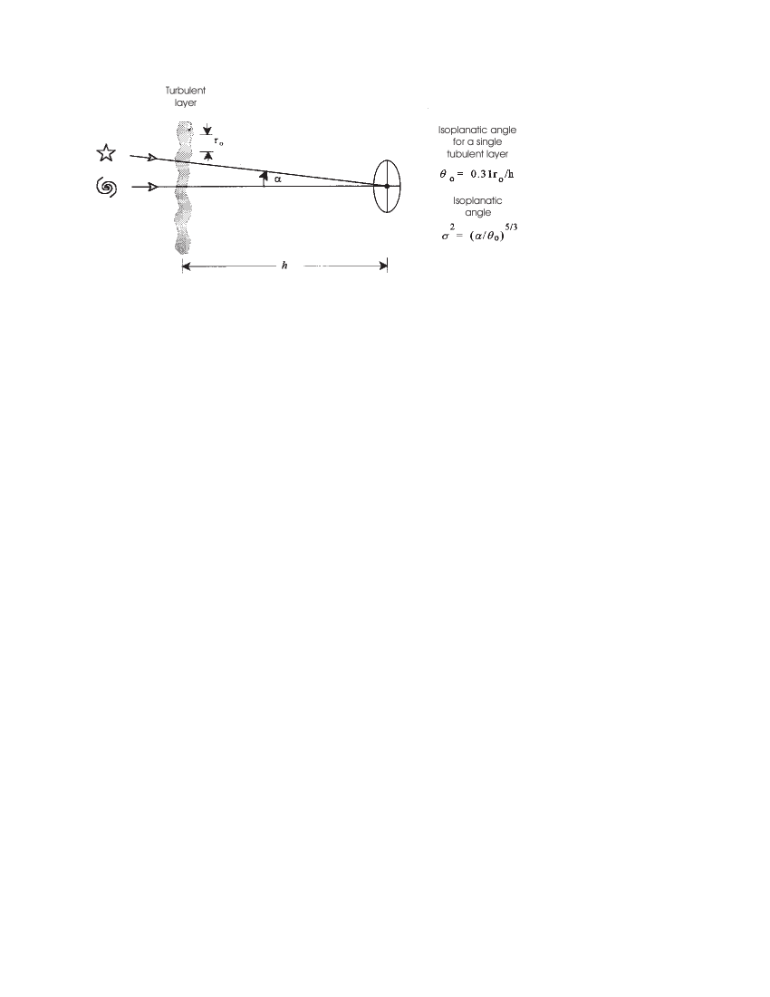
Figure 2.5: Angular anisoplanatism (Hardy, 1998).

Assuming a single turbulence layer at height $h$, $\theta_{0}=0.31r_{0}/h$, with $r_{0}$ being the correlation-length. The isoplanatic angle is very small, on average $\sim 2\hbox{${}^{\prime\prime}$}$ in the visual and up to $20\hbox{${}^{\prime\prime}$}$ in the near infrared.
The correction of the target degrades with the distance to the guide star and the PSF of the target star is elongated in the direction to the guide star.
In some cases the observed target can be used as a guide star itself. In astronomy though, most of the scientific interesting objects are faint or extended objects, like protoplanetary disks, star clusters or galaxies. In the case of protoplanetary disks as well as with observing exoplanets, the host star can mostly be used as guide star. Also in clusters one normally finds a suitable bright star. In the cases where no suitable guide star is close enough, artificial laser guide stars can possibly be used if implemented. This artificial sources are replacing the natural guide star as reference objects for the AO. So the sky-coverage can be enhanced by a huge factor. But laser guide stars are also introducing new problems, for example the cone-effect, which arises because of the finite distance of the laser focus point, which is produced in a height of 90 - 100 km by resonant fluorescence of a layer which is enriched with natural sodium atoms, and the therefore only cone-like sampling of the atmosphere (Bouchez et al., 2004). This effect is even more prominent in the case of the so-called Rayleigh laser beacons. These are produced in a height of 5 - 10 km by Rayleigh scattering of the laser radiation on atmospheric molecules (Fugate et al., 1991).

2.3 NACO

The instrument NACO is the adaptive optics system at the VLT and it is mounted at the UT4, Yepun, at the Nasmyth B focus (Lenzen et al., 2003; Rousset et al., 2003). It consists of two parts, the Nasmyth Adaptive Optics System NAOS and the High-Resolution Near IR Camera CONICA.

The overall tip and tilt of the wavefront is compensated by the tip-tilt plane mirror of NAOS. The higher order aberrations, including static aberrations of NAOS and CONICA, are compensated by the 185 actuators deformable mirror. A dichroic acts as the beam splitter to separate the light between CONICA and the WFS. There are several different dichroics, depending on whether the WF correction is done in the visible or the IR, how bright the guide star is and so on.
NAOS has two WF sensors, one operating in the visible and one in the near-IR. This kind of sensor consists of a lenslet array that samples the incoming WF. Each lens forms an image of the object and the displacement of this image from a reference position gives an estimate of the slope of the local wavefront at that lenslet. This WFS works with white light and also with extended sources and faint stars, although with a lower performance. For the visible sensor, two Shack-Hartmann sensors, one with a 14x14 lenslet array, with 144 valid sub-apertures and one with a 7x7 lenslet array and 36 valid sub-apertures are available and for the infrared sensor three Shack-Hartman sensors are available.
Anywhere within a $110\hbox{${}^{\prime\prime}$}$ diameter field of view an off-axis natural guide star can be selected, leading to a maximum distance between guide star and target of $55\hbox{${}^{\prime\prime}$}$. But due to the anisoplanatism the Strehl ratio is going down to $\sim 9\leavevmode\nobreak\ \%$ for a $V=10$ mag target with a separation to the guide star of $30\hbox{${}^{\prime\prime}$}$, observed in $\lambda=2.2\leavevmode\nobreak\ \mu m$ and a seeing of $0.8\hbox{${}^{\prime\prime}$}$, compared to a Strehl ratio of $\sim 47\leavevmode\nobreak\ \%$ for an on-axis target observed in the same wavelength and under the same seeing conditions.
If no suitable guide star is close enough to the target, a laser guide star (LGS) can be used. The PARSEC instrument is based on a 4W sodium laser guide star. The laser which is tuned on the $D_{2}$-line ($\lambda=589$ nm) of sodium, is focused at 90 km altitude where a thin, natural layer of atomic sodium exists. The backscattered light produces a $V\approx 11$ mag artificial guide star which is used for the AO correction.

The CONICA instrument is an IR imager and spectrograph in the wavelength range $1-5\leavevmode\nobreak\ \mu m$ and it is fed by NAOS. It is capable of imaging, long slit spectroscopy and coronographic and polarimetric observations. Several different plate scales are available, too.
For imaging, a variety of filters and pixel scales are offered. In principle three different plate scales and field of views (FoV) are available, plus one small FoV for spectral differential imaging (SDI). Table 2.1 lists the available cameras with their FoV, pixel scale and spectral range.

Camera	px-scale	FoV	Spectral
	[mas/px]	[arcsec]	range
S13	13.27	14 x 14	$1.0-2.5\leavevmode\nobreak\ \mu m$
S27	27.15	28 x 28	$1.0-2.5\leavevmode\nobreak\ \mu m$
S54	54.6	56 x 56	$1.0-2.5\leavevmode\nobreak\ \mu m$
SDI	17.32	5 x 5	$1.6\leavevmode\nobreak\ \mu m$
L27	27.19	28 x 28	$2.5-5.0\leavevmode\nobreak\ \mu m$
L54	54.6	56 x 56	$2.5-5.0\leavevmode\nobreak\ \mu m$

Table 2.1: List of available cameras for CONICA with plate scales, field of view and spectral range

Five broad band filters ($J,H,K_{s},L^{\prime},M^{\prime}$) and 29 narrow and intermediate band filters are available, plus two neutral density filters which can be combined with the other filters to reduce the flux of very bright sources.
The detector of CONICA is a Santa Barbara Research Center InSb Aladdin 3 array, with a net 1024 x 1024 pixels and a $27\leavevmode\nobreak\ \mu m$ pixel size. The wavelength range is from $0.8-5.5\leavevmode\nobreak\ \mu m$ and it has a quantum efficiency of 0.8 - 0.9. For bright objects, a number of ghosts become apparent (see Chap. 3.3).
A single integration with the detector corresponds to the Detector Integration Time (DIT) and the pre-processor averages $N$ of these exposures, NDIT, before the result is transferred to the disk. The number of counts in the final images always corresponds to DIT and not to the total integration time NDIT x DIT.
Three readout modes are offered. In case of the Uncorr mode the detector is reset and then read once. This mode is used when the background is high. The Double_RdRstRd mode is used when the background is intermediate between high and low and the detector array is read, reset and read again. If the background is low, the FowlerNsamp mode is used. Here the array is reset, read four times at the beginning of the integration ramp and four times at the end of the integration ramp.

A detailed description of the above mentioned characteristics of NACO and more information can be found in the NACO User’s Manual:
http://www.eso.org/sci/facilities/paranal/instruments/naco/doc/

2.3.1 Our Observation Configuration

In our observations, I used the visible dichroic with the 7x7 optical wavefront sensor and near-IR imaging with the narrow-band filter $NB\_2.12$ and the S27 camera. Due to the special arrangement of the stars in our FoV I calculated an own jitter pattern. For readout I chose the Double_RdRstRd mode with an integration time of 0.9 seconds for the target field and 0.4 seconds for the reference field. For more details see Chap. 3.3.

Chapter 3 Observations and Data Reduction

3.1 The Target Field

The target star I observed is an M2.5 V dwarf star in the solar neighborhood. GJ 1046 has an apparent magnitude of V = 11.61 mag and K = 7.03 mag and a stellar mass of $0.398\pm 0.007\leavevmode\nobreak\ \rm M\hbox{${}_{\odot}$}$. It is a high proper motion star with $\mu_{\alpha}=1394.10\leavevmode\nobreak\ \rm mas$ and $\mu_{\delta}=550.05\leavevmode\nobreak\ \rm mas$ and a parallax of 71.56 mas (i.e. a distance of 13.97 pc) (Perryman et al., 1997).
The companion orbiting GJ 1046 was found by radial velocity measurements with the UVES/VLT spectrograph within a search for planets around M dwarfs (Kürster et al., 2008, 2003; Zechmeister et al., 2009). In Figure 2 (from Kürster et al., 2008) the RV time series and best-fit Keplerian orbit of GJ 1046 is plotted. Assuming a stellar mass, from K-band mass-luminosity relationship (Delfosse et al., 2000), of $M=0.398\leavevmode\nobreak\ {\rm M\hbox{${}_{\odot}$}}$, a minimum companion mass $m_{\rm min}=26.9\leavevmode\nobreak\ {\rm M}_{\rm Jup}$ can be calculated for an inclination $i=90\hbox{${}^{\circ}$}$, corresponding to an edge-on view of the orbit and therefore measuring the maximum $RV$ amplitude, from the mass function $f(m)=(m\sin{i})^{3}/(M+m)^{2}=9.5\cdot 10^{-5}\leavevmode\nobreak\ M\hbox{${}_{\odot}$}$. Together with Equ. 1.2 for the $RV$ semi-amplitude $K$ an minimum orbital semi-major axis $a=0.42\leavevmode\nobreak\ {\rm AU}$ was inferred. Its mass and distance to the host star makes this companion a promising candidate for the brown dwarf desert. In Tab. 3.1 the stellar parameters and orbital characteristics inferred from the $RV$ measurements are listed. These parameters are kept fixed later in the astrometric orbit fit.

Table 3.1: Stellar and orbital parameters of GJ 1046

$RV$-derived parameters	value	uncertainty	units
$RV$ semi-amplitude K	1830.7	$\pm 2.2$	$ms^{-1}$
Period P	168.848	$\pm 0.030$	days
Eccentricity e	0.2792	$\pm 0.0015$
Longitude of periastron $\omega$	92.70	$\pm 0.50$	degree
Time of periastron $T_{p}$	3225.78	$\pm 0.32$	BJD-2 450 000
Mass function f(m)	9.504	$\pm 0.024$	$10^{-5}\leavevmode\nobreak\ M\hbox{${}_{\odot}$}$
Inferred parameters
Stellar Mass M	0.398	$\pm 0.007$	$M\hbox{${}_{\odot}$}$
Minimum companion mass $m_{min}$	26.85	$\pm 0.30$	$M_{Jup}$
Min. semi-major axis of companion orbit a	0.421	$\pm 0.010$	AU
Critical inclination  $i_{crit}$	20.4		degree
Probability for $i<i_{crit}$	6.3%
a for $m=0.08\leavevmode\nobreak\ M\hbox{${}_{\odot}$}$

To exceed the upper brown dwarf mass limit of $0.08\leavevmode\nobreak\ \rm M\hbox{${}_{\odot}$}$ the orbital inclination would have to be smaller than $20.4.\hbox{${}^{\circ}$}$ (or larger than $159.6\hbox{${}^{\circ}$}$). But the probability that the inclination angle $i$ is by chance smaller than this value, $p(90\hbox{${}^{\circ}$}\geq i\geq\theta)=\cos{\theta}$ is only 6.3%, assuming random orientation of the orbit in space. Combining the RV data with the HIPPARCOS astrometry of GJ 1046 (Kürster et al., 2008); (see also (Reffert and Quirrenbach, 2006)) a $3\leavevmode\nobreak\ \sigma$ upper limit to the companion mass of $112\leavevmode\nobreak\ M_{Jup}$ was determined. The probability for the companion to exceed the star/BD mass threshold ($0.8\leavevmode\nobreak\ M\hbox{${}_{\odot}$})$ is just 2.9 %. These two constraints make it very unlikely that the companion is stellar, but it rather is a true brown dwarf desert companion.
The expected minimum astrometric signal (see Equ. 1.8) due to the companion is 3.7 mas peak-to-peak, which corresponds to 0.136 pixel on the NACO S27 detector. This value is calculated using the HIPPARCOS parallax of 71.56 mas and holds for the case that the orientation of the system is such that one only sees and measures the minor axis, $2*b_{1}$ of the orbit. But the true effect is possibly much larger. For an object at the brown dwarf/star border the full minor axis would extend 11.5 mas or 0.42 px and the full major axis 12.1 mas, as the orbit is not very eccentric. At the HIPPARCOS derived upper limit for the mass of $112\leavevmode\nobreak\ M_{Jup}$, it would be $2*b_{1}=15.4\rm\leavevmode\nobreak\ mas$ or 0.57 px. This is one of the rare cases where a spectroscopic star-substellar compaion system comes into reach for astrometric observations.

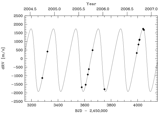
Figure 3.1: RV time series of GJ 1046 from Kürster et al. (2008). The solid line corresponds to the Keplerian solution with a period of 169 d. Note that the average measurement error is $3.63\leavevmode\nobreak\ {\rm ms}^{-1}$, much smaller than the plot symbols. Additional RV measurements with ESO/FEROS from the last years fit very well with this orbit, showing that the signal is indeeed due to a companion orbiting the star.

For astrometric measurements a reference star, preferably close to the observed star is needed. By chance GJ 1046 is located at $\sim 30\hbox{${}^{\prime\prime}$}$ separation from a suitable reference star, see Fig. 3.3 and 3.2. This reference star, 2MASS 02190953 -3646596, has V = 14.33 and K = 13.52 (colors taken from the 2MASS/SIMBAD, catalogues) which makes it from its color V-K = 0.81 an F2 star with an effective temperature of 6̃750 Kelvin (Tokunaga, 2000). Assuming the star to be a main sequence star, one can infer an absolute magnitude in the visual of $M_{V}=3.7$ mag from theoretical isochrones (Marigo et al., 2008) and use the distance modulus $m-M=-5+5\log{\big{(}r[pc]\big{)}}$ to estimate a distance for the reference star of $\sim 1337$ pc. At this distance the star would have a parallax movement of only $\sim 0.75$ mas. Also interstellar reddening occurs at such distances, which makes the color of the star redder, so in reality it is even bluer and therefore further away. So I do not expect a strong influence on the relative parallax between the two stars compared with the parallax of GJ 1046 alone in my measurements within the aimed precision. Also the proper motion of the reference star is not expected to be very high and I therefore use the HIPPARCOS values for the proper motion and parallax of GJ 1046 as a good first estimate for the results in the fit later.

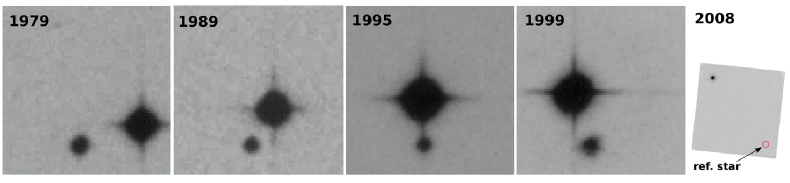
Figure 3.2: Time series of the movement of GJ 1046 on the sky over nearly 30 years. Due to its high proper motion it passes the star which now is used as the reference star in this work. The first, third and fourth image is taken from the SuperCosmos Sky Survey (SSS), the second one from the ESO archive and the last image is one of my own observations with NACO.

3.2 The Reference Field

Adaptive optics corrections during an observation are not constant. It is a dynamical process, whose performance depends on the atmospheric conditions during the observation and changes of these conditions. Also the telescope focus may have changed between two observing epochs, inducing a slightly changed platescale. I rotated the FoV with the derotator, to fit the star asterism onto the detector, but this rotation only has a finite accuracy. To check and calibrate for such effects, I observed a reference field in the rim of the globular cluster 47 Tucanae. This field contains more stars than our target field and is observed very close in time to the target field. It is used to measure the change in platescale between the different epochs. I do not need to know the absolute platescale, but its change between the single epochs must be determined to attain subpixel accuracy. Also the accuracy of the rotation of the detector was monitored with the reference field, to adopt a reasonable error for the rotation angle to our data in the target field. To correct for the uncertainty in the rotation is not possible, because the de-rotator is turned back to the zero position when moving the telescope to the reference field and a fixation of the rotated instrument to the angle of the target field was not possible in service mode, either.
I chose the reference field in the old globular cluster 47 Tucanae, because of its large distance of $4.0\pm 0.35$ kpc (McLaughlin et al., 2006) and accordingly with it the small intrinsic movement of the single stars in the field. The velocity dispersion of the inner parts of the cluster is 0.609 mas in the plane of the sky and the dispersion in the outer parts being slightly smaller (McLaughlin et al., 2006). The reference field contains three bright stars and several fainter ones suitable to check the image scale and the field rotation, see Fig. 3.3, right.

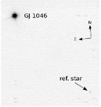
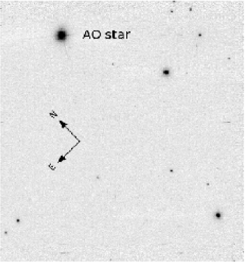
Figure 3.3: NACO image of GJ 1046 (left) and the reference field in the globular cluster 47 Tucanae (right) from July 2008. GJ 1046 is the bright star in the upper left corner, the reference star is located in the lower right corner. Also visible in the frames are ghosts produced by the bright star (elongated features, see Chap. 3.3).

As far as possible I checked the cluster membership of the stars in the field. But for some, especially the faint ones, it was impossible as no 2MASS magnitudes exist, so that I could not confirm their membership via the color-magnitude diagram. McLaughlin et al. observed 47 Tuc with the Hubble Space Telescope (HST) and calculated proper motions and stellar dynamics for the stars in the core of the cluster (McLaughlin et al., 2006). Unfortunately our field lies just outside their radius around the core, where they obtained their high precision measurements. However, they also observed the outer part of the cluster where our field lies and did not mark any of the stars in their tables, meaning they have not measured an uncommon hich velocity compared to the mean cluster motion for these stars. Also, comparing the positions of the single stars in the different epochs in our NACO images did not show any unusual or large motion of one of the stars in one direction. I therefore assume all the stars in the observed reference field to be cluster members with common proper motion.
The asterism in the reference field was chosen to be similar to the configuration of the AO and reference star in our target field plus additional stars for computing the necessary field distortions between the single epochs. For that I had to rotate the FoV by $42\hbox{${}^{\circ}$}$ anticlockwise. Altogether I used 11 stars for the final fit of $x$ and $y$-shift, -scale and rotation between the epochs.

3.3 Adaptive Optics Observations of GJ 1046

The adaptive optics observations of GJ 1046 analyzed here were carried out with the adaptive optics instrument NAos COnica (NACO) at the Very Large Telescope (VLT) of the European Southern Observatory (ESO) with the UT4 Yepun telescope. All observations were executed in Service Mode within a monitoring program from July 2008 till October 2009 to derive the true mass of the companion via astrometric measurements. Altogether I obtained 10 epochs, where the first nine are in roughly three week intervals between July and December 2008 and the last epoch was obtained end of September 2009, see table 3.2 for an overview of the observations. The last row is an indicator for the quality of the data: A = good, B = mostly within specifications, C = outside specifications; with the observing specifications of: seeing better than 0.8^′′ and airmass lower than 1.6. In the target field, GJ 1046 itself was used as the AO guide star, in the reference field the brightest star in the upper left corner was used for wavefront sensing.

Epoch	Date	Target Field		Ref. Field		# jitter	# images per	Quality
		DIT	NDIT	DIT	NDIT	position	position
1	03/07/08	0.9	110	0.4	10	5	5	A
2	02/08/08	0.9	110	0.4	10	5	5	B
3	22/08/08	0.9	110	0.4	10	5	5	C
4	24/08/08	0.9	110	0.4	10	5	5	A
5	27/09/08	0.9	110	0.4	10	5	5	B
6	30/10/08	0.9	122	0.4	10	5	5	A
7	18/11/08	0.9	122	0.4	10	5	5	B
8	07/12/08	0.9	122	0.4	10	5	5	B
9	27/12/08	0.9	122	0.4	10	5	5	B
10	30/09/09	0.9	120	0.4	15	5	5	B

Table 3.2: Overview over the observations, with exposure time, number of jitter positions and quality indicator of the obtained data.

The target star is not visible from the Paranal Observatory between February and June, or only at very high airmass. But as the orbital period of the companion is 169 days, I covered a full orbit between July and December 2008 (epochs 1-9). This was very important to better distinguish the parallactic motion from the half year orbital motion. It was planed to obtain two more epochs in the period between July and September 2009 to better constrain the orbit, but I only got the last epoch in October 2009, which was still important to extend the time baseline for constraining the relative proper motion between GJ 1046 and the reference star. In Fig. 3.4 the observations are shown distributed over one year in the left panel and over one orbital period in the right panel. The plotted ellipses are simulations of the motion of GJ 1046 with parallactic motion, but without proper motion: in the left panel for inclination $i=30\hbox{${}^{\circ}$}$ and ascending node $\Omega=150\hbox{${}^{\circ}$}$ (dashed line), $i=45\hbox{${}^{\circ}$},\leavevmode\nobreak\ \Omega=60\hbox{${}^{\circ}$}$ (solid line) and pure parallax movement without any orbital motion (dotted line). The red squares represent the times of observations overplotted over the simulated motion with $i=45\hbox{${}^{\circ}$},\leavevmode\nobreak\ \Omega=60\hbox{${}^{\circ}$}$, with the number denoting the corresponding epoch. This plot shows how important it is to have a proper sampling of observations to distinguish the orbital motion from the parallax movement. The right panel shows the times of observations overplotted over a simulated orbit with $i=45\hbox{${}^{\circ}$},\leavevmode\nobreak\ \Omega=60\hbox{${}^{\circ}$}$ and proper motion and parallax subtracted. As one can see, the full orbit is coverd by the observations. The open blue square marks the periastron passage, $T_{0}=54745.41$. (Fig. 3.3).

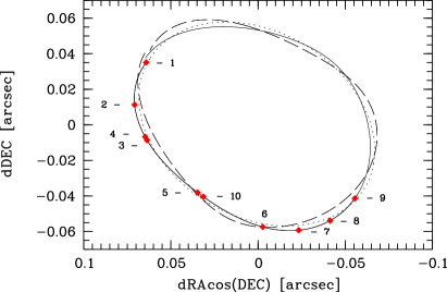
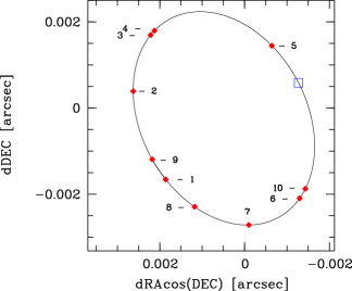
Figure 3.4: GJ 1046 observations distributed over one year in the left panel and over one orbital period in the right panel. In the left panel, the ellipses are simulations with $\varpi=71.56$ and $i=30\hbox{${}^{\circ}$},\leavevmode\nobreak\ \Omega=150\hbox{${}^{\circ}$}$ (dashed line), $i=45\hbox{${}^{\circ}$},\leavevmode\nobreak\ \Omega=60\hbox{${}^{\circ}$}$ (solid line) and pure parallax movement without any orbital motion (dotted line), proper motion has been subtracted. The right panel shows a simulation of an orbit with $i=45\hbox{${}^{\circ}$},\leavevmode\nobreak\ \Omega=60\hbox{${}^{\circ}$}$ and parallax and proper motion subtracted. The red squares represent the times of observations overplotted on the simulated orbits, with the number denoting the corresponding epoch. The open blue square marks the periastron passage, $T_{0}=54745.41$.

The DIT values were chosen, such that the peak counts for the bright star in each field are $\leq 80\%$ of the detector linearity limit of $110,000\leavevmode\nobreak\ e^{-}$ for a small seeing of $0.4\hbox{${}^{\prime\prime}$}$. For the star in the field with the highest separation from the AO guide star I estimated a signal-to-noise (S/N) value integrated over the stellar disk and a formal astrometric precision using photon statistics $(\sigma/(S/N))$ for a seeing of $0.8\hbox{${}^{\prime\prime}$}$. All the performance estimates were made with the NAOS preparation software and the NACO ETC (Exposure Time Calculator). In Tab. 3.3 the estimated performance for an observation in the middle of the epochs is listed.

The observations were made with a narrow-band filter centered on $2.12\leavevmode\nobreak\ \mu m$ and with a FWHM of $0.022\leavevmode\nobreak\ \mu m$ to minimize the effects of differential atmospheric dispersion. The reference field in 47 Tuc was observed each epoch immediately before the science field. I observed the reference field before the target field and not after it, for reasons of visibility of the two fields. 47 Tuc culminates roughly half an hour before GJ 1046 at the location of the Paranal Observatory, hence the conditions were best for both fields when observed in this order.
As one can see in Fig. 3.3 left, the target star GJ 1046 and the reference star just fit in the FoV of the S27 camera of the NACO instrument. GJ 1046 lies in the upper left corner of the detector and the astrometric reference star in the lower right corner when the detector is rotated by $6\hbox{${}^{\circ}$}$ anticlockwise. I chose this camera because of its, for the purpose of this work, suitable pixel-scale of 27 mas/px. I aimed for a precision of 0.5 mas and with the presumption of an accuracy of 1/50 pixel this camera was the one best suited of the three offered ones, as the FoV of the S13 camera is too small.
To avoid a badpixel coincident at the pixel positions of the stars and to better calculate the sky-background, a jitter pattern is necessary for observations in the infrared. Preferable is a pattern with an offset of several arcseconds in different directions, which is difficult with this arrangement of the stars on the detector.

Field	Strehl$[\%]$			FWHM$[$mas$]$			Encircled energy$[\%]$			S/N	$\Delta$
	$0.4\hbox{${}^{\prime\prime}$}$	$0.6\hbox{${}^{\prime\prime}$}$	$0.8\hbox{${}^{\prime\prime}$}$	$0.4\hbox{${}^{\prime\prime}$}$	$0.6\hbox{${}^{\prime\prime}$}$	$0.8\hbox{${}^{\prime\prime}$}$	$0.4\hbox{${}^{\prime\prime}$}$	$0.6\hbox{${}^{\prime\prime}$}$	$0.8\hbox{${}^{\prime\prime}$}$	@ $0.8\hbox{${}^{\prime\prime}$}$	[mas]
GJ1046	53.1	47.8	41.1	72	72	73	59.4	54.6	48.6	-	-
ref	39.7	21.3	7.6	76	87	132	48.6	31.7	16.0	142	0.39
47 Tuc	54.4	49.9	44.4	71	72	73	60.6	56.5	51.7	-	-
field	45.5	30.1	14.6	74	79	94	53.3	39.6	23.7	351	0.11
a @ indicated seeing

Table 3.3: Performance estimates for the middle epoch observation. Calculated for the AO star and the star furthest away from it. The last column lists the astrometric precision $\Delta$ of the fainter star which is $30.14\hbox{${}^{\prime\prime}$}$ separated from GJ 1046 in the target field and $21.28\hbox{${}^{\prime\prime}$}$ separated from the AO star in the reference field 47 Tuc. All the performance estimates were made with the NAOS preparation software and the NACO ETC.

Another problem occurred, because of the brightness of the target star. Bright stars are known to produce a number of electronic and optical ghost features on the NACO detector, depending on their position on the detector. When the position of a bright star is $(xs,ys)$, the electronic ghosts appear approximately at the positions $(1024-xs,ys)$, $(xs,1024-ys)$ and $(1024-xs,1024-ys)$. The last one of these would appear very close to our faint reference star and could therefore influence the positional measurement. An optical ghost which looks like a set of concentric rings may also appear, but I did not see that in the data.
Special care has been taken to calculate a jitter pattern which made sure both stars are always within the FoV and at least 5 sigma afar from the detector edges or any ghost. Because the whole configuration plus the additional jitter pattern brings the two stars close to the edges of the detector, I had to make sure that the reference star was always located on the very same pixel at the beginning of the observations, so the calculated jitter pattern assures a successful observation. In Table 3.4 the position of GJ 1046, the reference star and the closest ghost are listed together with the final jitter pattern, which is shown in Fig. 3.5. I had to differ the last jitter point in the observations of the reference field due to the different positions of the stars and the ghosts of the bright star in this field.

rel. jitter offset	GJ 1046		Ghosts		Ref. star		Dist. to	Dist. to
x [′′]     y [′′]	x [px]	y [px]	x [px]	y [px]	x [px]	y [px]	ref star [px]	ref star [$\sigma$]
0        0	156	854	868	170	917	65	115.8	9.3
1        0.5	193	873	831	151	954	83	140.1	11.2
0        2	193	946	831	78	954	157	145.6	11.7
-1        0.5	156	965	868	59	917	175	125.5	10.0
0       -1.5	119	946	905	78	880	157	82.4	6.6

Table 3.4: Positions of the bright target star, the ghost it is producing closest to the reference star and the distance of the ghost to the reference star.

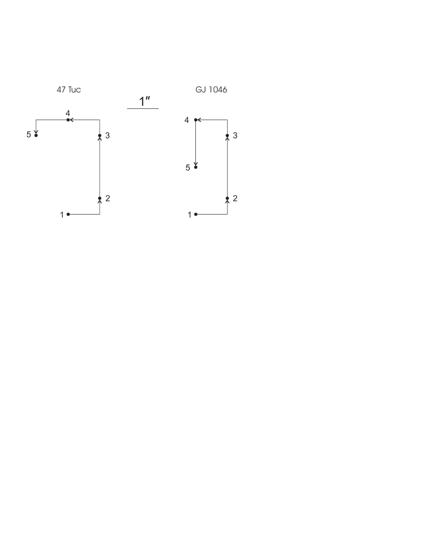
Figure 3.5: Jitter pattern for the target and reference field.

3.4 Data Reduction

I did not use the NACO-pipeline products for our astrometric measurements. Instead I reduced the data on our own. The data reduction is the same for the target and the reference field. So I only describe the principle chain here and name differences directly when they occur.
First I created a badpixel-mask using the badpixel routine included in the eclipse data reduction package. This routine uses the flatfield images to create the badpixel mask. If possible and available I used the badpixel masks created by ESO from sky-flats taken in the same night and in the same filter as our observations. But this was only the case for two observations. In the other cases the dome-flats were used. The mask was then combined with the hotpixel mask, created by ESO during the pipeline data reduction. The so derived strange-pixel mask is then used to correct the flaged pixels with the median of their 8 nearest neighbors in the science frames as well as the dark current frames.
Then the dark frames were multiplied by the gain factor of the S27 camera detector, which is 11 e/ADU. Masterdarks were created by median combining darks with the same exposure times as the target and reference frames respectively.
Also the dome-flats are multiplied by the gain. The masterdark for the target field and the reference field are then subtracted for the corresponding data reduction. Flats with lamps on and flats with lamps off were median combined, respectively, and the off-flat was subtracted from the on-flat. Finally the obtained flat field image is normalized by dividing it through its mean value.
Now I have everything to reduce the science data following the standard technique. The single frames are multiplied by the gain, masterdark subtracted and divided by the normalized flat field. Finally the frames are corrected for the strange-pixels.

3.4.1 Sky Subtraction

I investigated the subtraction of the sky-background in different ways. As I do not have additional sky images I created a sky frame from median combining all science frames in the first step. But this left me with some ’holes’ close to the stars after subtracting the sky frame from the science frames. This is due to the small jitter pattern I used during the observations and the fact that I only have 5 different jitter positions. A bigger and therefore better pattern was not possible, see Chap. 3.3. Light from the wings of the stars is not averaged out and produces somewhat higher values in the sky frame, which then appear as holes in the sky subtracted science frames.
The second step was to remove the influence of the stars by using $\kappa-\sigma$ clipping. If the mean of a single science frame is significantly higher than the median value of the sky created before in step one, pixels in the science frame with values higher or lower than a certain range around the mean, the stars, are substituted by the mean of the pixels left after the $\kappa-\sigma$ clipping. These frames, cleaned for stars, are then used to calculate the sky by median combination of them.
I tested this procedure for different ranges around the mean value, which define the pixels which are substituted. The holes indeed were less pronounced, but they also were more irregular, which introduced a strange pattern into the wings of the PSF of the bright star. This degrades the possibility to measure accurately the position of the stars and I decided not to create the sky this way.
Another test was made by creating the sky only by median combining an inner part of the science frames, where there are no stars. But this did not lead to a huge improvement in the sky subtraction either.
I decided finally to not subtract the sky background at all, as it is not very high and does not show any slope over the frames. It can be therefore assumed as a local constant background which should not disturb the astrometric measurements.

3.4.2 50 Hz Noise

The reduced frames showed a strong noise pattern along the rows. This phenomenon is known as 50 Hz noise and was found to be caused by the fans in the front end electronics of the Infrared Array Control Electronics (IRACE). One can decrease the effect by subtracting the median of each row from the very same row. I created a frame with the same size as the science frames in which the values in the rows have the median value of the corresponding science row. I created the median value not over the whole row, but detector quadrant wide. With this I took care of the fact, that the NACO detector of the S27 camera is read out quadrant wise.

3.4.3 Shift and Add

Now the frames are fully reduced. The frames obtained on the same jitter position are added. This is possible because the telescope was not moved between the single frames of one jitter position. I am left with five frames per epoch and field. These frames are added by simple shift and add using the jitter routine (Devillard, 1999). So I have one frame per target and reference field for every epoch. I also tested shifting and adding all single frames, but this gave no better result than adding the five already stacked frames from the different jitter positions.

Chapter 4 Analysis and Astrometric Corrections

Several corrections have to be applied to the measured positions of the stars before fitting the astrometric orbit. These include converting pixel coordinates to celestial coordinates, differential refraction, differential aberration and change in plate-scale and detector rotation. Logically, these corrections are executed in the inverse order as they appear. The detector distortions have to be corrected as first step in principle, as it is the last effect which results in a displacement in position of the stars on the detector. But to avoid cross-talk between this effect and displacements from aberration and refraction, I corrected for the differential refraction and aberration before. First the differential refraction has to be corrected as it deflects the light rays after the aberration already occurred, then the aberration is corrected. In an iterative way the correction of the detector distortion measured as third step, is applied to the originally measured detector positions of the stars before correction for refraction and aberration. After that, the correction for differential refraction and differential aberration is performed again. Fig. 4.1 shows the stepwise and iterative corrections which are described in the following sections in detail.

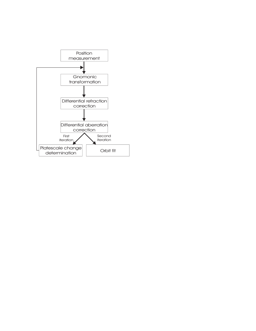
Figure 4.1: Stepwise description of the corrections applied to the measures pixel coordinates of the stars.

4.1 Position Measurements

The positions of the stars were measured by fitting a Moffat-function to the individual stars using the non-linear least square fitting package MPFIT2DPEAK, written in the IDL language and provided by Craig Markwardt (Markwardt, 2009). The Moffat function is a modified Lorentzian with a variable power law index $\beta$ (Moffat, 1969). It better represents the form of a PSF corrected by AO than a simple Gaussian-function, but the Gaussian-function is contained in the Moffat-function as a limiting case with $\beta\rightarrow\infty$:

$$f(x,y)=c+I_{0}\leavevmode\nobreak\ \left[\left(\frac{x-x_{0}}{\rho_{x}}\right)^{2}+\left(\frac{y-y_{0}}{\rho_{y}}\right)^{2}+1\right]^{-\beta}$$ (4.1)

c is a constant, $x_{0},y_{0}$ are the center of the function and $\rho_{x},\rho_{y}$ define the FWHM of the PSF: $FWHM_{x}=\rho_{x}(2\frac{1}{\beta}-1)^{1/2}$. The Moffat-function has two advantages over the Gaussian. It is numerically well behaved in the treatment of narrow PSFs, because of the use of polynomials instead of exponential expressions. But it also allows the wings of the PSF to be fitted. This makes it a better fitting function for AO corrected PSFs.
For the PSF-fit, the stars in the stacked frames were marked and a small box of $15\times 15$ px ($407\times 407$ mas) was cut around them. After finding the px with the maximum, a bigger box with $31\times 31$ px ($842\times 842$ mas) was cut around the star. Then the Moffat was fitted to the PSF. I also tried to just fit the Center of Weight (CoW), but the fitted CoW of the distribution is dependent on the box size, whereas the fitted Moffat peak was very stable for all kinds of box-sizes. I therefore decided to fit a rotated Moffat-function to determine the peak position of the PSFs.
A phenomenon in adaptive optics images which occurs for sources which are not the guide star, is known as radial breathing. The PSFs of the objects are elongated in the direction to the guide star, but not in the direction perpendicular to it. The effect gets stronger the farther away a source is from the guide star, so the shapes of the PSFs get more and more elliptical. This is important to know for photometry, but should not influence the center of the distribution.
The fit routine also outputs values for the Full Width at Half Maximum (FWHM). I could have used this for an estimate of the positional error, if I assumed photon statistics. But to also cover the error, which may arise from the fit itself, I adopted another method for the positional uncertainty.

4.1.1 Positional Error Estimate - Bootstrapping

To estimate the positional error resulting from the fit, I re-sampled the intensity distribution in the cut boxes, PSF plus background, 100 times with the bootstrap method and fitted each single realization again with a Moffat-function. The bootstrap method is a general technique for estimating for example standard errors for estimators and was first introduced by Bradley Efron (Efron, 1979). I numbered all photons in each PSF distribution and generated the same amount of random numbers. The random numbers defined which of the photons was picked and put at the same position in the re-sampled PSF. But after that, the photon is 'put back', so it could be picked up again. To do so, one needs to know the total number of photons, $N_{ph}$, in the box. To get that number, one has to take into account the gain-factor of the detector, ($11\leavevmode\nobreak\ e^{-}/ADU$ for NACO), and the fact that the images are averaged twice. First during the acquisition, when N frames with the exposure time DIT are averaged, and then when the frames are stacked to obtain the final frame (2.3 and 3.4.3). Because of the massive rising computational amount when multiplying the averaged image by NDIT, the number of photons is a lot larger, and because I did not want to underestimate the error, I decided to stay conservative and worked on the averaged image without multiplying by NDIT. Only the gain and the average factor from adding the single frames is taken into account. In this way I generated the re-sampled PSFs by executing the pick and put-back procedure as many times as there were photons in the original distribution. This was done 100 times for each star in the target field as well as in the reference field.
The standard deviations in x and y of the 100 fits from the mean position are used as an estimate for the errors.
To check whether the obtained fitting errors are reasonable, I also fitted a rotated Gaussian distribution to the same PSFs in the boxes and calculated the positional error if we only assume photon statistics, $dx=\frac{\sigma_{x}}{\sqrt{N_{ph}}}$. The errors are of the same order as the ones from the bootstrap re-sampling, but due to the fact that a Gaussian does not represent the form of the AO corrected PSFs very well and that I wanted to include the error contribution of the fit, I used the errors from the bootstrap re-sampling as the positional uncertainties. In Table 4.1 the errors from the bootstrapping and the Gaussian approximation are listed.
Additionally to this error one has to take into account the errors originating from the differential refraction, differential aberration and the plate-scale and rotational errors. These contributions to the error budget are described in the following sections.

			Bootstrap error		Gauss error
			x	y	x	y
		[px]	$2.62\cdot 10^{-4}$	$2.48\cdot 10^{-4}$	$2.15\cdot 10^{-4}$	$2.02\cdot 10^{-4}$
	AO star	[mas]	$7.11\cdot 10^{-3}$	$6.73\cdot 10^{-3}$	$5.84\cdot 10^{-3}$	$5.48\cdot 10^{-3}$
GJ 1046		[px]	$0.70\cdot 10^{-2}$	$0.73\cdot 10^{-2}$	$1.64\cdot 10^{-2}$	$1.61\cdot 10^{-2}$
	ref star	[mas]	0.19	0.70	0.45	0.44
		[px]	$5.48\cdot 10^{-4}$	$5.96\cdot 10^{-4}$	$3.70\cdot 10^{-4}$	$3.47\cdot 10^{-4}$
	AO star	[mas]	0.01	0.02	0.01	$9.42\cdot 10^{-3}$
47 Tuc		[px]	$1.63\cdot 10^{-2}$	$1.60\cdot 10^{-2}$	$1.31\cdot 10^{-2}$	$1.14\cdot 10^{-2}$
	ref star	[mas]	0.44	0.43	0.36	0.31

Table 4.1: Positional error from the PSF fit calculated with bootstrap re-sampling and simple photon statistics. In the 47 Tuc reference field, the star furthest away in the opposite corner of the detector is used as the reference star (ref star).

4.2 Astrometry with FITS-Header Keywords

4.2.1 World Coordinates in FITS

World coordinates are coordinates that serve to locate a measurement, as for example frequency, wavelength or longitude and latitude, in a multidimensional parameter space. The representation of world coordinates in the Flexible Image Transport System (FITS), which is used by all observatories since the General Assembly of the IAU (resolution R11), was first introduced by Wells et al. (1981). This initial description was very simple and Greisen and Calabretta (2002) later described it in more detail with more possible extensions. Keywords in the FITS header are used to describe the parameters necessary to convert the $x$ and $y$ coordinates from the detector into the world coordinates. Each axis of the image has a certain coordinate type and a reference point, for which the coordinate value, the pixel coordinate and an increment are given. The basic keywords are:
CRVALn coordinate value at reference point CRPIXn pixel coordinate at reference point CDELTn coordinate increment at reference point CTYPEn axis type

To convert pixel coordinates to world coordinates a multi-step process is needed, whose principle steps are shown in Fig. 4.2.

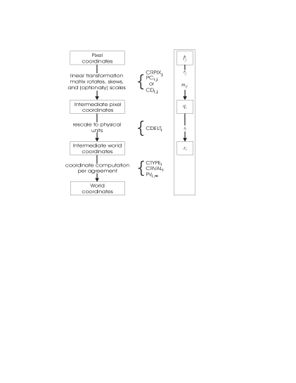
Figure 4.2: Conversion of pixel coordinates to world coordinates (after Calabretta and Greisen (2002)).

The first step is a linear transformation via matrix multiplication from the pixel coordinates $p_{j}$ to intermediate pixel coordinates $q_{i}$:

$$q_{i}=\sum_{j=1}^{N}m_{ij}(p_{j}-r_{j})$$ (4.2)

$r_{j}$ are the pixel coordinates of the reference point, given by the CRPIX_j elements. In the following notation the index $j$ refers to the pixel axis and $i$ to the world coordinate axis. The $m_{ij}$ matrix is a non-singular square matrix with the dimension of $N\times N$. $N$ is given by the keyword value of NAXIS, which gives the dimension of the data array, but not necessarily that of the world coordinates. If the dimensions of the World Coordinate System (WCS) are different, the keyword WCSAXES is used, which then gives the maximum value of the index of any WCS keyword. The resulting intermediate pixel coordinates $q_{i}$ are offsets from the reference point along axes that are coincident with those of the intermediate world coordinates $x_{i}$. The transformation to the corresponding $x_{i}$ is then a simple scaling:

$$x_{i}=s_{i}q_{i}$$ (4.3)

There are two formalisms that describe the transformation matrix in FITS. One is the PCi_j, where the matrix elements of $m_{ij}$ are given by the PCi_j header keywords and $s_{i}$ by CDELTi. If PCi_j and CDELTi are not given in the FITS header, the second formalism is used. This one combines Eqs. 4.2 and 4.3 to :

$$x_{i}=\sum_{j=1}^{N}(s_{i}m_{ij})(p_{j}-r_{j})$$ (4.4)

with the keywords CDi_j$=s_{i}m_{ij}$. This formalism omits the second step on the transformations.
The last step depicted in Fig. 4.2 from the intermediate world coordinates to the world coordinates applies a non-linear transformation, depending on the world coordinate system one is aiming at.

4.2.2 Celestial Coordinates in FITS

For the transformation to celestial coordinates, the intermediate world coordinates are interpreted as Cartesian coordinates in the plane of the projection. The final step is divided into two steps which are a spherical projection defined in terms of a convenient coordinate system, the native spherical coordinates, and a spherical rotation of these coordinates to finally obtain the required celestial coordinates (Calabretta and Greisen, 2002). Depending on the kind of projection, the equations for the transformation to the native longitude and latitude $(\phi,\theta)$ are specified in the keyword CTYPEi. There is a wide variety of projecting a sphere onto a plane and vice versa. The one used in data set of this work is the so-called gnomonic projection. It is described in more detail in Sec. 4.2.3. The values of the keywords are:
CTYPE1 = ’RA - - - TAN’ CTYPE2 = ’DEC - - TAN’

The last three characters define the projection type and the leftmost four characters are used to identify the celestial coordinate system. In this case a gnomonic projection (4.2.3) and equatorial coordinates.
For the last step, the spherical rotation from native coordinates to celestial coordinates, one needs three Euler angles which specify the rotation. The celestial coordinates for the reference point, $(\alpha_{0},\delta_{0})$, specified in the header via the CRVALi keyword, are associated with a native coordinate pair $(\phi_{0},\theta_{0})$, which are defined explicitly for each projection. The difference of these native coordinates for different projections is due to the fact that the projections diverge at different points. The Mercator projection diverges for example at the native pole, while the gnomonic one diverges at the equator. Therefore they cannot have the reference point at these points, because that would mean infinitive values for CRVALi. The projection equations are then constructed in a way so that $(\phi_{0},\theta_{0})$ transform to the reference point $(x,y)$.
There are several other FITS keywords which define the necessary astrometry:
RADECSYS defines the reference frame, e. g. FK5 EQUINOX defines the coordinates epoch, e. g. 2000.0 MJD-OBS defines the Modified Julian Date of the observation start

The combination of CTYPEi, RADECSYS and EQUINOX define the coordinate system of the CRVALi and of the celestial coordinates resulting from the transformations.

4.2.3 Transformation from xy-Coordinates into RA/DEC

To convert the pixel values measured for the peak positions of the stars in the frames to celestial coordinates, I used the astrometry in the FITS header. The projection given by the keyword CTYPEi is a special form of a zenithal projection, the gnomonic projection. The name deduces from the Greek word Gnomon $(\gamma\nu\acute{o}\mu o\nu)$, which stands for a shadow-stick used as an astronomical instrument. The shadow cast by the tip of the stick was already used to measure the time with a sundial in antiquity. The gnomonic projection is the oldest map projection, developed by Thales in the 6th century BC.
The gnomonic projection displays all great circles on a sphere as straight lines. The surface of the sphere is projected from its center, hence perpendicular to the surface, onto a tangential plane and the least distortions occur at the tangent point. In Astronomy, the Earth’s radius is small compared to the distance to the stars and can be neglected, so the observatory can be seen as being in the center of the projection. This directly implies the negligence of the diurnal parallax (see Chap. 4.3.10).

A problem occurred after stacking the images with the jitter routine, as described in Chap. 3.4.3. The image obtained is slightly larger in $x$- and $y$-direction than the single images before. The new size of the image is updated in the FITS header by the jitter routine, but not the resulting coordinate shift of the reference point. Additionally, no information is given on how much the zero-point of the array is shifted. To compute the new pixel coordinates of the reference point in the stacked image, I had to execute some more steps.
As the star I used as a guide star for the AO system is quite bright and also very well corrected in the single frames I could measure its pixel coordinates very accurately. I measured its position in the first stacked image of the first jitter position in the same way as described in Chap. 4.1. Then I calculated the distance to the given coordinates for the reference point. After measuring all positions in the final image, I recalculated the pixel coordinates of the reference point by using the beforehand calculated distance to the AO guide star and updated the CRPIXi values in the FITS header.

The transformation of the coordinates was then performed with the IDL routine xyad.pro from the IDL astrolib which uses the formalism described in detail in paper II of the series of papers describing coordinates in the FITS formalism (Calabretta and Greisen, 2002).

4.3 Astrometric Corrections

The exact position where an object appears on the sky does not only depend on the coordinates of the observed object, but also on various effects which are connected to the relative velocity of the observer, i.e. the aberration, and the atmosphere of the Earth, i.e. the atmospheric refraction.

4.3.1 Theory of Atmospheric Refraction

The atmospheric refraction decreases the true zenith distance of an object. Light, passing a surface that separates two layers with different refractive indices $n$ and $n+dn$ is refracted in a way described by Snell’s Law. Let $\eta$ be the angle of incident in a medium with refractive index $n$. The angle of refraction in a medium with refractive index $n+dn$ is then $\eta+d\eta$ following

$$(n+dn)\sin{(\eta+d\eta)}=n\sin{\eta}$$ (4.5)

The total bending of the light can be expressed as

$$R=z_{t}-z_{0}$$ (4.6)

where $R$ is the total refraction angle experienced by the light ray, $z_{t}$ the true zenith distance in degrees and $z_{0}$ the apparent observed zenith distance. In the infrared wavelength regime, the refraction can reach tens of arcseconds, where the effect is larger in the J-Band than in the K-Band.
In theory one needs to know $n$ at all points of the light-path through the atmosphere to determine $R$. In practice this is normally not possible and one has to represent the atmosphere by a model which leaves $R$ only as a function of atmospheric conditions.
Using a spherical model for the atmosphere means assuming iso-refractive index spheres around the center of the Earth.

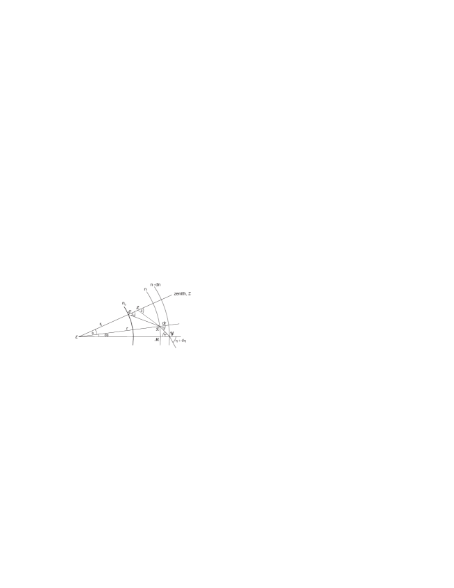
Figure 4.3: Refraction in the atmosphere. For more details see text.

In figure 4.3, $r_{0}$ is the geocentric distance of the observer $\mathcal{O}$ from the center of the Earth $\mathcal{E}$, $n_{0}$ the refractive index at ground level and $z_{0}$ the apparent distance of an celestial object to the local zenith $\mathcal{Z}$.
If one considers a small layer with width $dr$ and the refractive index $n$, then the range $\mathcal{XY}$ is the linear path of the light ray coming from the observed object through this layer. At the point $\mathcal{Y}$ one can apply Snell’s law to the incoming light ray which comes from a medium with the refractive index $n-dn$. $\eta+d\eta$ is then the incident angle in the point $\mathcal{Y}$ and $\Psi$ the refractive angle. This leads to:

$$n\sin{\Psi}=(n-dn)\sin{(\eta+d\eta)}$$ (4.7)

Naming the angle between the two zenith directions of the observer and the one in point $\mathcal{X}$, $\phi$, the increment of this angle towards the direction $\mathcal{M}$, $d\phi$ and the radius vector from $\mathcal{E}$ to $\mathcal{X}$, $r$, one can write:

$$r\sin{\eta}=(r+dr)\sin{\Psi}$$ (4.8)

This equation comes from the sine relation in the triangle $\mathcal{EXY}$.
If one now multiplies respectively the right and left sides of 4.7 and 4.8 one gets

$$nr\sin{\eta}=(r+dr)(n-dn)\sin{(\eta+d\eta)}$$ (4.9)

Again with Snell’s law this proves $nr\sin{\eta}$ to be invariant. Transformed to the observer’s position and together with Equ. 4.7 one can write the important relation:

$$nr\sin{\Psi}=n_{0}r_{0}\sin{z_{0}}$$ (4.10)

If one looks at the triangle $\mathcal{LEX}$ one can see that $z=\phi+\Psi$ and from the triangle $\mathcal{XMY}$ one gets $\tan{\Psi}=\frac{rd\Phi}{dr}$. Combining these two equations one gets

$$dz=d\Psi+\frac{\tan{\Psi}}{r}dr$$ (4.11)

Now one first differentiates 4.10, which yields

$$nr\cos{\Psi}d\Psi+r\sin{\Psi}dn+n\sin{\Phi}dr=0$$ (4.12)

or written in a different way

$$nr\cos{\Psi}\left(d\Psi+\frac{dr}{r}\tan{\Psi}\right)=-r\sin{\Psi}dn$$ (4.13)

Together with Equ. 4.11 one has:

$$dz=-\frac{dn}{n}\tan{\Psi}$$ (4.14)

Now one can look at Equ. 4.10 in a different way and write it, with $nr\cos{\Psi}=\sqrt{r^{2}n^{2}-r^{2}_{0}n^{2}_{0}\sin^{2}{z_{0}}}$, as:

$$\tan{\Psi}=\frac{r_{0}n_{0}\sin{z_{0}}}{\sqrt{r^{2}n^{2}-r^{2}_{0}n^{2}_{0}\sin^{2}{z_{0}}}}$$ (4.15)

This one substitutes into the previously obtained Equ. 4.14 and finally derives after integration over dz

$$R=r_{0}n_{0}\sin{z_{0}}\leavevmode\nobreak\ \int_{1}^{n_{0}}\frac{dn}{n(r^{2}n^{2}-r_{0}^{2}n_{0}^{2}\sin^{2}{z_{0}})^{1/2}}$$ (4.16)

This general refraction formula requires a detailed knowledge of the refractive index $n$ and therefore for the whole atmosphere itself, as $n$ depends on the wavelength $\lambda$ of the incoming light and the temperature $T$, pressure $P$ and water pressure $P_{w}$ of the atmosphere. This formula is an exact description of the refractive index of the air and can be calculated numerically if the variation of the refractive index with height, $r=r(n)$, is postulated. However, a simplification is possible when only modest zenith distances are allowed. One can then expand Equ. 4.16 to (Green, 1985; Gubler and Tytler, 1998):

$$R=A\tan{z_{0}}+B\tan^{3}{z_{0}}$$ (4.17)

$A$ and $B$ are constants and depend on the wavelength $\lambda$, $T$, $P$ and the relative humidity $H$. This expansion makes the calculation of the differential refraction a lot easier, see next section.

4.3.2 Differential Atmospheric Refraction

The differential atmospheric refraction between two stars, $\Delta R$, is due to two main effects: The different color of the stars (meaning different temperature of the stars and therefore different effective wavelength in the used filter) and the different zenith distance of the two stars. The color dependent effect is smaller (around 20 times) than the effect due to the differing zenith distances for moderate zenith distance differences of $\sim 15\hbox{${}^{\prime\prime}$}$ and temperature differences of $\sim 3000$ Kelvin in the K, K’ and H band (Gubler and Tytler, 1998). Assuming two stars with refraction $R_{1}$ and $R_{2}$ respectively, $\Delta R=R_{1}-R_{2}$, and an apparent zenith distance difference of $\Delta z_{0}=z_{1}-z_{2}$, one can write the refraction experienced by star 2 expressed by $z_{1}$ and $\Delta z_{0}$ and (4.17) as:

$$\begin{split}R_{2}(z_{2})&=R_{2}(z_{1}-\Delta z_{0})\\ &=A_{2}\tan{(z_{1}-\Delta z_{0})}+B_{2}\tan^{3}{(z_{1}-\Delta z_{0})}\end{split}$$ (4.18)

Expanding this equation around $z_{1}$ to second order in $\Delta z_{0}$ then yields

$$\Delta R=\Delta R_{\lambda}+\Delta R_{z}$$ (4.19)

where $\Delta R_{\lambda}$ denotes the color dependent effect and $\Delta R_{z}$ the differential zenith distance dependent effect. The two components of $\Delta R$ have the form:

$$\Delta R_{\lambda} =(A_{1}-A_{2})\tan{z_{1}}+(B_{1}-B_{2})\tan^{3}{z_{1}}$$ (4.20)

$$\Delta R_{z} =(1+\tan^{2}{z_{1}})\bigl{(}(A_{2}+3B_{2}\tan^{2}{z_{1}})\Delta z_{0}$$

$$-\left[A_{2}\tan{z_{1}}+3B_{2}(\tan{z_{1}}+2\tan^{3}{z_{1}})\right]\Delta z_{0}^{2}\bigr{)}$$ (4.21)

Usually the constants $A$ and $B$ are determined empirically. Gubler and Tytler did this by first changing the integration variable in Equ. 4.16 from $n$ to $z$ which yields

$$R=-\int_{0}^{z_{0}}\frac{rdn/dr}{n+rdn/dr}\leavevmode\nobreak\ dz$$ (4.22)

Full integration of this integral for two different zenith distances yields the refraction indices corresponding to these two values of $z$. A curve fit to Equ. 4.22 then gives the two constants $A$ and $B$. I am using characteristic but fixed values for the atmospheric parameters hereafter, so the constants $A$ and $B$ are only dependent on the wavelength:

$$T_{0} =278\leavevmode\nobreak\ \rm K$$

$$P_{0} =800\leavevmode\nobreak\ \rm mbar$$

$$H_{0} =10\leavevmode\nobreak\ \%$$

One can then derive an expression for $A$ and $B$ in seconds of arc with only a wavelength dependence. This was done by Gubler and Tytler (Gubler and Tytler, 1998) empirically for the K-Band (centered on $2.2\leavevmode\nobreak\ \mu m$):

$$A(\lambda) = 45.95126+\frac{0.26147}{\lambda^{2}}$$ (4.23)

$$B(\lambda) = -0.05083862-\frac{0.0002622385}{\lambda^{2}}$$ (4.24)

I used during the observations a narrow-band filter centered at $2.12\mu m$. So we could suppress and therefore neglect the color dependent part of the differential refraction, $\Delta R_{\lambda}$, and only corrected for the effect due to the different zenith distances of the stars, $\Delta R_{z}$. With $\lambda=2.12\mu m$, the two constants then take the values $A=46.0094\hbox{${}^{\prime\prime}$}$ and $B=-0.050897\hbox{${}^{\prime\prime}$}$.
Looking at Equ. 4.21 one can see that even with the most extreme values during the observations, $\Delta z_{0}=17.2\hbox{${}^{\prime\prime}$}$ and $z_{1}=48\hbox{${}^{\circ}$}89$, the quadratic term never exceeds $\sim 1.26\leavevmode\nobreak\ \mu as$. The following expression for $\Delta R_{z}$ is therefore a good approximation:

$$\Delta R_{z}=\frac{(1+\tan^{2}{z_{1}})(A_{2}+3B_{2}\tan^{2}{z_{1}})}{206265}\Delta z_{0}$$ (4.25)

The factor in the denominator comes from the fact that $\Delta z_{0}$ is now expressed in arcseconds instead of radians. Also, $\Delta R_{z}$ is now expressed in seconds of arc.

As stated above, the values for $A$ and $B$ are calculated for fixed standard values of atmospheric temperature, pressure and humidity, $T_{0},P_{0},H_{0}$. But in reality, the actual circumstances during the observations are different. Depending on how much the actual temperature, pressure and humidity vary from these standard values, the differential refraction changes, too. Gubler and Tytler (1998) investigated this phenomenon and gave values for the change in $\Delta R$ due to changes differences of temperature, pressure and humidity form the standard values. The relation between the parameters is linear, the differential refraction goes as the inverse of the ground-level temperature and changing the pressure by a given fraction changes $\Delta R$ by the same fraction. A change in the humidity does not change the differential diffraction significantly. Changing the humidity from 10% to 100% only leads to a change in the differential refraction of a few micro-arcseconds.
While I took the change in temperature and pressure into account, I did not correct for any change in the humidity, as it was close to the standard value of 10% anyway during all observations. The correction factors were taken into account as follows. Taking the values given by Gubler and Tytler (tables 3 and 4) I made a linear least-squares approximation in one-dimension to the data, yielding values for the slope $m$ and the interception point with the y-axis $b$ for the relation between temperature and diff. refraction and pressure and diff. refraction, respectively:

$$\Delta R_{T} =m_{T}\cdot\Delta T+b_{T}$$ (4.26)

$$\Delta R_{P} =m_{P}\cdot\Delta P+b_{P}$$ (4.27)

Here $\Delta T$ is the difference to $T_{0}$ in Kelvin, $\Delta P$ the difference to $P_{0}$ in mbar and $\Delta R$ is given in percent. The derived values for $m$ and $b$ are: $m_{T}=-0.363\pm 0.049$, $b_{T}=0.086\pm 0.409$, $m_{P}=0.125\pm 0.018$ and $b_{P}=0.000\pm 0.380$. After converting the changes in $\Delta R$ from percentage to arcseconds, the final differential refraction is given by:

$$\Delta R=\Delta R_{z}+\Delta R_{T}+\Delta R_{P}$$ (4.28)

4.3.3 Correction for Differential Refraction

With the results from Equs. 4.25 and 4.28, one can start to correct the measured positions of the stars for differential refraction. As this is the last distortion before the light arrives on the detector, it has to be corrected first and before the differential aberration.

The celestial coordinates given for the reference point in the FITS header are already refraction and aberration corrected. So one only has to correct for the differential part of the refraction between the reference point and the stars. This is done by first undoing the aberration correction for the reference point (see Chapter 4.3.5), so that one knows at which point the light rays really entered the atmosphere. With these ’new’ coordinates for the reference point, the celestial coordinates of the stars are calculated in the way described in Chapter 4.2. Then the zenith distances $z_{0}$ of the reference point and the stars are given by:

$$\cos{z_{0,i}}=\sin{\delta_{i}}\sin{\varphi}+\cos{\delta_{i}}\cos{\varphi}\cos{HA_{i}}$$ (4.29)

Here $\varphi$ denotes the local latitude of the observatory, which is for the VLT/UT4  $\varphi=-24\hbox{$.\!\!^{\circ}$}6270$, $\delta$ the declination of the star and $HA=LST-\alpha$ the local hour angle of the star. $i$ stands for the different stars. As the zenith distance changes with time, $HA$ and $z_{0}$ were calculated over the whole observing time of one epoch. This means for every single frame of the field in that epoch, which leaves me with 25 (35 for epoch 1, see Tab. 3.2) values for $HA$ and $z_{0}$ for each night. I therefore introduce another index, $j$, which stands for the different frames at an individual epoch.

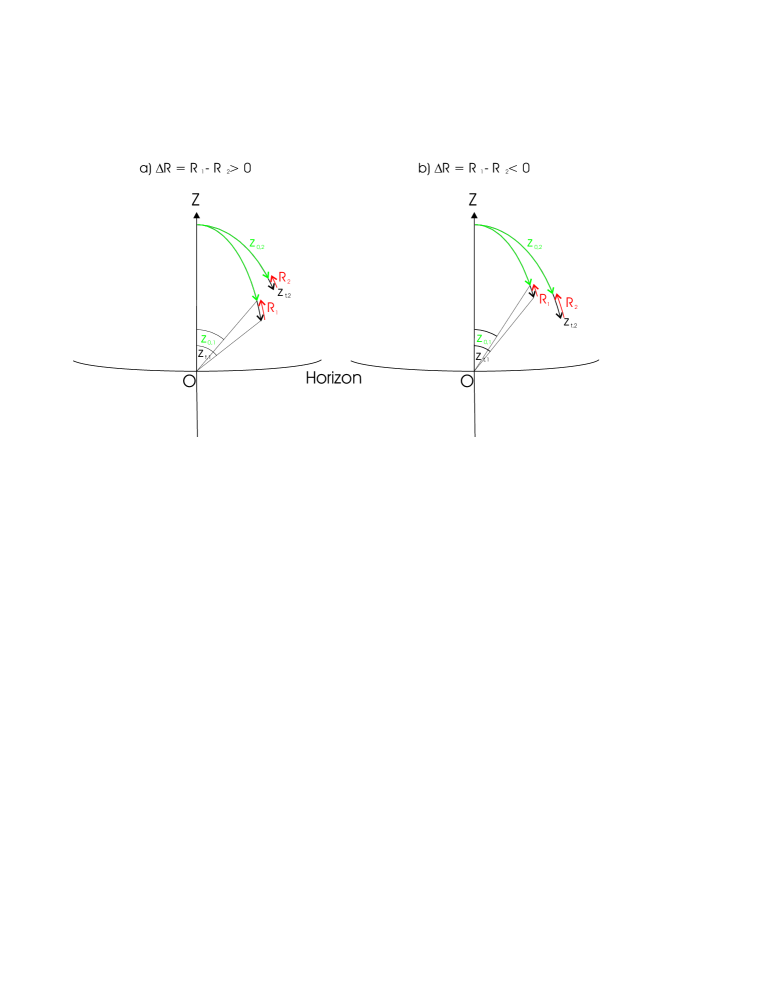
Figure 4.4: Differential refraction

Now one can calculate $\Delta z_{0_{i,j}}=z_{0_{ref,j}}-z_{0_{i,j}}$, and after that $\Delta R_{i,j}$ for each star, using Equ. 4.28 and $z_{1}=z_{0_{ref,j}}$ in Equ. 4.25. $\Delta T$ was in the range between 3.72 and 8.71 K, and $\Delta P$ between -57.3 and -54.7 mbar for all epochs. I calculated $\Delta R_{T{i,j}}$ and $\Delta R_{P{i,j}}$ for each frame in each epoch with the parameters $m_{T},m_{P},b_{T}$ and $b_{P}$ derived from the linear fits. The sign of $\Delta z_{0}$ and therefore $\Delta R$ depends on the time the observation was conducted and therefore the orientation of the star asterism on the local sky relative to the reference point. If the zenith distance $z_{0_{ref}}$ of the reference point is bigger than the zenith distance of any star $z_{0_{i}}$, then $\Delta z_{0_{i}}\leavevmode\nobreak\ \textgreater\leavevmode\nobreak\ 0$ and also $\Delta R_{i}\leavevmode\nobreak\ \textgreater\leavevmode\nobreak\ 0$ for this star. If $z_{0_{ref}}\leavevmode\nobreak\ \textless\leavevmode\nobreak\ z_{0_{i}}$ then $\Delta z_{0_{i}},\Delta R_{i}\leavevmode\nobreak\ \textless\leavevmode\nobreak\ 0$. In Figure 4.4 a and b, the two cases are shown. Depending on whether the observation was carried out before, after, close to or even during the passing of the stars through the local meridian, the time-depending behavior of $\Delta z_{0_{i}}$ and all the following parameters is different. In Fig. 4.5 one can see different cases during different phases of the visibility of the stars. Plotted as the solid curve is the difference in altitude of the two stars in the field: Alt(reference star) - Alt(GJ 1046). The dotted curve shows the visibility of the objects above the local horizon at Paranal Observatory in mid-October. The right $y$-axis gives the altitude in degrees. The vertical dashed line marks the time of the local Meridian Passage of GJ 1046. Due to the slightly different coordinates of the two objects, they overtake each other during the night, leading to a change in the sign of the differential refraction correction. The reference point of the detector, to which the differential refraction is measured, lies between the two stars. The small inlets show the configuration of the two stars at different phases of their visibility; the left one, when the reference star is at a lower altitude, the middle one when they are nearly at the same height above the horizon and the right on when GJ 1046 is at a lower altitude. Also shown are the times of observation in LST (in blue) for all individual epochs.

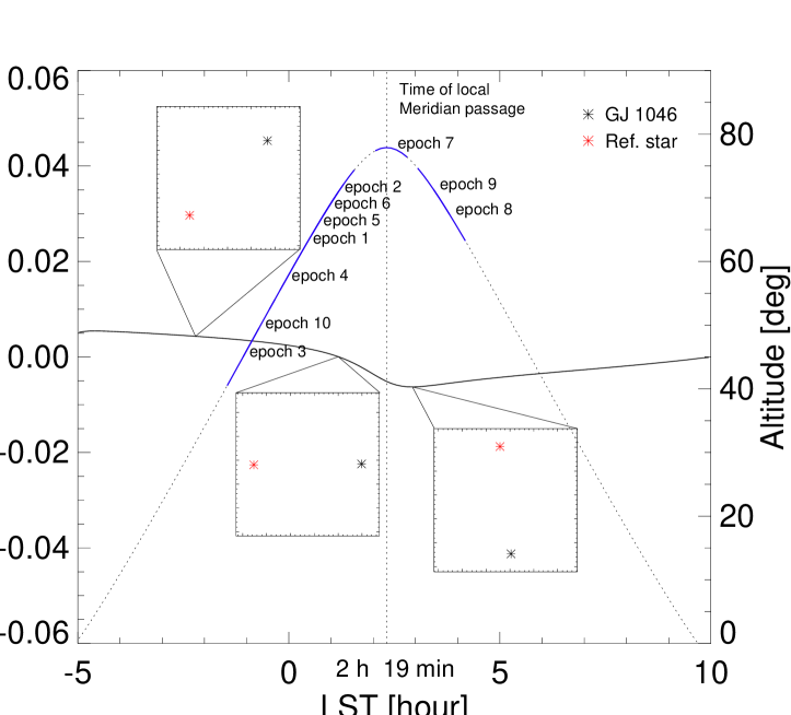
Figure 4.5: Sign of the differential refraction correction during different times of observations. Plotted as the solid curve is the difference in altitude of the two stars in the field: Alt(reference star) - Alt(GJ 1046). The dotted curve shows the visibility of the objects above the local horizon at the Paranal Observatory in mid of October. The right x-axis gives the altitude in degree. The vertical dashed line marks the time of the local Meridian Passage of GJ 1046. The small inlets show the orientation of the two stars at different phases of their visibility; the left one, when the reference star is at a lower altitude, the middle one when they are nearly at the same height above the horizon and the right on when GJ 1046 is at a lower altitude. Also shown in blue are the times of observation in LST for all epochs.

The true zenith distance of the stars is then:

$$z_{t_{i,j}}=z_{0_{i,j}}+\Delta R_{i,j}$$ (4.30)

Now one needs to recalculate $\alpha$ and $\delta$ of the stars. Here the fact that the refraction changes the zenith distance, but not the azimuth of the stars helps. The azimuth $AZ$ of a given frame in a given observation for a star is:

$$\cos{AZ}=\frac{(\sin{\delta}-\cos{z_{0}}\sin{\varphi})}{\sin{z_{0}}\cos{\varphi}}$$ (4.31)

Rearranging this equation and replacing $z_{0}$ with $z_{t}$ lets one calculate the declination corrected for differential refraction:

$$\delta_{corr_{i,j}}=\sin^{-1}\left({\cos{z_{t_{i,j}}}\sin{\varphi}+\sin{z_{t_{i,j}}}\cos{\varphi}\cos{AZ_{i,j}}}\right)$$ (4.32)

To compute the right ascension one needs to recalculate the hour angle $HA$ first, as $\alpha_{i,j}=LST_{j}-HA_{i,j}$:

$$HA_{i,j}=\cos^{-1}\left(\frac{\cos{z_{t_{i,j}}}-\sin{\delta_{corr_{i,j}}}\sin{\varphi}}{\cos{\delta_{corr_{i,j}}}\cos{\varphi}}\right)$$ (4.33)

From this I calculated offsets from the positions in right ascension and declination $(\alpha,\delta)$ without the differential refraction correction:

$$\Delta\alpha_{i,j}=\alpha_{i,j}-\alpha_{corr_{i,j}}$$ (4.34)

Again I had 25 (35) values of $\Delta\alpha$ for each star. To get one value for correction I calculated the mean change in position, $\Delta\alpha_{i}=\frac{\sum_{\scriptstyle j=1}^{\scriptstyle N}\Delta\alpha_{i,j}}{N}$, N = 25 (35), same for $\delta$, and the corresponding error of the mean value, $\sigma_{\alpha_{i}}/\sqrt{N},\leavevmode\nobreak\ \sigma_{\delta_{i}}/\sqrt{N}$, where $\sigma_{\alpha_{i}}$ and $\sigma_{\delta_{i}}$ are the standard deviations of the $\Delta\alpha_{i,j}$ and $\Delta\delta_{i,j}$. The coordinates corrected for differential refraction are then derived by:

$$\alpha_{corr_{i}} = \alpha_{i}-\Delta\alpha_{i}$$ (4.35)

$$\delta_{corr_{i}} = \delta_{i}-\Delta\delta_{i}$$ (4.36)

In Tab. 4.2 the corrections in right ascension and declination are listed for the two stars in the target field for each epoch. Now one has the coordinates of the stars corrected for differential refraction. The next step is then to correct for differential aberration.

	GJ 1046		reference star
epoch	$\Delta\alpha$ [mas]	$\Delta\delta$ [mas]	$\Delta\alpha$ [mas]	$\Delta\delta$ [mas]
1	$0.678\pm 0.141$	$-0.126\pm 0.023$	$-1.891\pm 0.149$	$0.510\pm 0.009$
2	$-0.006\pm 0.066$	$0.043\pm 0.037$	$-0.441\pm 0.010$	$0.195\pm 0.046$
3	$3.553\pm 0.099$	$-0.034\pm 0.019$	$-5.740\pm 0.149$	$0.057\pm 0.030$
4	$1.782\pm 0.061$	$-0.272\pm 0.004$	$-3.114\pm 0.092$	$0.478\pm 0.010$
5	$1.998\pm 0.059$	$-0.275\pm 0.006$	$-1.898\pm 0.087$	$0.531\pm 0.005$
6	$0.349\pm 0.068$	$-0.122\pm 0.025$	$-0.993\pm 0.103$	$0.393\pm 0.028$
7	$0.248\pm 0.141$	$2.123\pm 0.068$	$-0.358\pm 0.184$	$-2.732\pm 0.109$
8	$2.902\pm 0.021$	$1.186\pm 0.046$	$-4.251\pm 0.041$	$-1.733\pm 0.063$
9	$2.780\pm 0.039$	$1.540\pm 0.057$	$-3.960\pm 0.066$	$-2.186\pm 0.047$
10	$3.475\pm 0.101$	$-0.172\pm 0.017$	$-4.743\pm 0.132$	$0.237\pm 0.024$

Table 4.2: Differential refraction corrections applied to the two stars in the target field. Values are given for correction in right ascension and declination plus the error arising from the change in zenith distance of the stars during the observation. The total differential effect between the two stars is the difference between their values.

4.3.4 Errors from Differential Refraction Correction

Correcting for differential refraction can introduce several error terms:

• The first one, which we already showed, is the error coming from neglecting the quadratic term in Equ. 4.21. This error is even for our most extreme observation configurations only $\sim 1.26\leavevmode\nobreak\ \mu as$ and well below our aimed precision.
  

• Another error source are the not perfectly known celestial coordinates of the stars to calculate $z_{0}$. Although the given absolute coordinates may not have a precision better than a few arcseconds, this is no problem as the error in the differential refraction is only about $\sim 5\leavevmode\nobreak\ \mu as$ if the zenith distance $z_{0}$ is only known to a precision of $0\hbox{${}^{\circ}$}01=36\hbox{${}^{\prime\prime}$}$ (Gubler and Tytler, 1998). This is well within the pointing accuracy of the VLT. Also, I am not aiming for absolute astrometry to obtain the orbital motion due to the companion, but instead only need relative astrometry to the reference star in the image.
  

• The biggest error term comes from the linear fit made to calculate the correction factors due to different temperature and pressure during the observations. The deviation of the data from a linear relation can be used to calculate errors for the derived slope and intersection values, which then lead to errors of the correction factor in $\Delta R$ of $\sim 0.5-1.0$%. This translates into a small error of the calculated $\Delta\alpha_{ij}$ and $\Delta\delta_{ij}$. The errors for the coordinate offsets $\Delta\alpha_{i}$ and $\Delta\delta_{i}$ are then calculated by $\sqrt{1/\sum_{\scriptstyle j=1}^{\scriptstyle N}\frac{1}{\sigma_{i,j}}}$, where $\sigma_{i,j}$ stands for the single errors of the $\Delta\alpha_{ij}$ and $\Delta\delta_{ij}$. The errors arising from this fit are between 0.129 - 1.779 mas for $\Delta\alpha_{i}$ and between 0.050 - 0.313 mas for $\Delta\delta_{i}$. The large upper limit results from one epoch, where the temperature and pressure values were deviating a lot stronger than at the other observing epochs. The errors of all other epochs are below the milli-arcsecond range. Still the errors resulting from the correction due to differing atmospheric conditions are pretty high and probably need a better model to correct for if one wants to go down to small micro-arcsecond precision.

• Additional errors arise from the change of the zenith distance during the observation. The observations took around 45 min for the target field, which lead to a change in zenith distance depending on the time of observation, before, close to or after the crossing of the targets through the local meridian. The result is a variation of $z_{0}$ between 0.5^∘ in the best case (epoch 7) and 16.1^∘ in the worst case (epoch 1), which translates into $0.35-2.29\rm\leavevmode\nobreak\ mas$ peak-to-peak difference in the correction $\Delta\alpha_{ij}$ and $0.07-0.98\rm\leavevmode\nobreak\ mas$ in $\Delta\delta_{ij}$ for the different epochs. The larger the zenith distance the stronger the refraction, because of the higher airmass the light has to travel through. The error from calculating the mean value for $\Delta\alpha_{i}$ and $\Delta\delta_{i}$ varies therefore between $21-184\leavevmode\nobreak\ \mu as$ and $4-109\leavevmode\nobreak\ \mu as$ for right ascension and declination, respectively, see also Tab. 4.2.
  This error and the error from the correction necessary due to the different temperature and pressure are taken into account by quadratic addition with the error from the PSF-Fit.

4.3.5 Theory of Aberration

The observer’s velocity through space relative to an observed object is responsible for a phenomenon called Bradley aberration or Stellar aberration. It was discovered by James Bradley in 1727 (Bradley, 1727). He was trying to measure the stellar parallax of g Draconis, in order to confirm the Copernican theory of the Solar System, as it proves the motion of the Earth. Instead he measured an annual variation which was not consistent with the expected parallax. The variation was strongest for stars in the direction perpendicular to the orbital plane of the Earth. As $\gamma$ Draconis passes right through the zenith in Greenwich, where Bradley did his observations, it was by chance a perfect target to detect stellar aberration. Bradley concluded rightly that the displacement he saw was not due to changes in the Earth’s position, but rather due to changes in Earth’s velocity. The aberration is caused by the relative velocity of the source, e.g. star, and the observer and the finite speed of light during the light travel time. The relative positions between the observer on Earth and the source change and the light seems to be coming from a direction different from the direction from which it was emitted. The movement of the observer can be divided into three different motions leading to the following three effects:

• The diurnal aberration caused by the daily rotation of the Earth

• The annual aberration, due to the movement of the Earth around the barycenter of the Solar System

• The secular aberration due to the motion of the Solar System barycenter in space

The secular aberration is a displacement due to the relative motion of the stars and the Solar System barycenter and is equal to the proper motion of the stars multiplied by the light time. Since this is rarely well known and the barycentric position of a star is mostly of marginal interest, this effect is normally ignored.
The absolute effect of the annual aberration can be approximated by

$$A_{year}\approx k_{year}\sin{\theta}$$ (4.37)

Here $k=V/c\approx 10\leavevmode\nobreak\ km\leavevmode\nobreak\ s^{-1}/300000\leavevmode\nobreak\ km\leavevmode\nobreak\ s^{-1}\approx 20.5\hbox{${}^{\prime\prime}$}$ is the annual aberration constant and $\theta$ is the angle between the velocity vector of the Earth and the direction of the light coming from the star, see Fig. 4.6. The differential effect between two stars at a separation of 30^′′ can then reach up to 3 mas over one year and needs to be corrected for. The differential effect of the diurnal aberration is smaller, around $42\leavevmode\nobreak\ \mu as$ per day.
But to derive and correct the effect of the aberration precisely one needs to take the relativistic addition of velocities into account, where the distinction between annual and diurnal aberration is not possible. This is done by applying the Lorentz transformation between two sets of coordinates, $x,y,z,(\mathbf{r})$ and time $t$ in a given reference frame $S$, and $x^{\prime},y^{\prime},z^{\prime},(\mathbf{r^{\prime}})$ and $t^{\prime}$ in another frame $S^{\prime}$ which is moving with the constant velocity $\mathbf{V}$ with respect to $S$. The generalized Lorentz transformation from the moving frame to the stationary one can then be written as:

$$\mathbf{r} =\mathbf{r^{\prime}}+\gamma\mathbf{V}t^{\prime}+(\gamma-1)\frac{\mathbf{V}(\mathbf{V}\cdot\mathbf{r^{\prime}})}{V^{2}}$$ (4.38)

$$t =\gamma\left(t^{\prime}+\frac{\mathbf{V}\cdot\mathbf{r^{\prime}}}{c^{2}}\right)$$ (4.39)

here $\gamma=(1-V^{2}/c^{2})^{-1/2}$, is the Lorentz factor. A point $\mathbf{r}$ in the stationary system $S$ has the velocity $\mathbf{U}=\text{d}\mathbf{r}/\text{d}t$. In the moving system its coordinates are $\mathbf{r^{\prime}},t^{\prime}$ and its velocity would be $\mathbf{U^{\prime}}=\text{d}\mathbf{r^{\prime}}/\text{d}t^{\prime}$. Now one can differentiate Equ. 4.39:

$$\frac{\text{d}\mathbf{r}}{\text{d}t} =\frac{\text{d}\mathbf{r^{\prime}}}{\text{d}t^{\prime}}\frac{\text{d}t^{\prime}}{\text{d}t}+\gamma\leavevmode\nobreak\ \mathbf{V}\frac{\text{d}t^{\prime}}{\text{d}t}+(\gamma-1)\left(\mathbf{V}\cdot\frac{\text{d}\mathbf{r^{\prime}}}{\text{d}t^{\prime}}\frac{\text{d}t^{\prime}}{\text{d}t}\right)\frac{\mathbf{V}}{V^{2}}$$ (4.40)

$$\text{d}t =\gamma\left(\text{d}t^{\prime}+\left(\mathbf{V}\cdot\frac{\text{d}\mathbf{r^{\prime}}}{\text{d}t^{\prime}}\text{d}t^{\prime}\right)/c^{2}\right)$$ (4.41)

And with the new notation

$$\frac{\text{d}t^{\prime}}{\text{d}t}=\frac{1}{\gamma(1+\mathbf{V}\cdot\mathbf{U^{\prime}}/c^{2})}$$ (4.42)

one can than write:

$$\mathbf{U}=\frac{\mathbf{U^{\prime}}+\gamma\mathbf{V}+(\gamma-1)(\mathbf{V}\cdot\mathbf{U^{\prime}})\mathbf{V}/V^{2}}{\gamma(1+\mathbf{V}\cdot\mathbf{U^{\prime}}/c^{2})}$$ (4.43)

This is the formula one needs to correct for aberration.

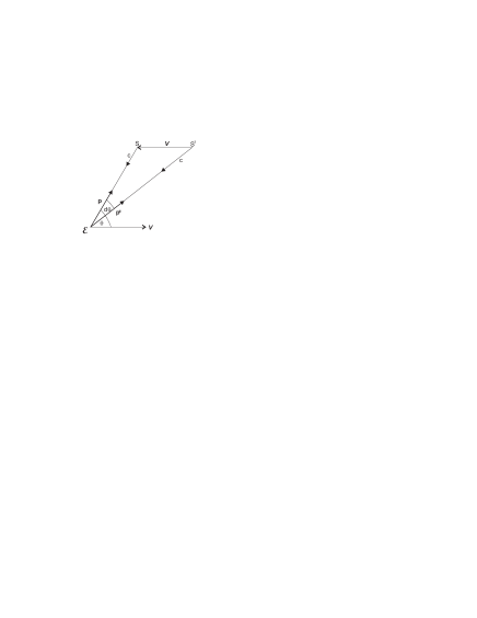
Figure 4.6: Stellar aberration

Now one can apply this result to the case of the moving Earth. The velocity of the Earth, $\mathcal{E}$ with respect to the stationary stars is $\mathbf{V}$. In Fig. 4.6, the unit vector $\mathbf{p}$ is in the direction to the geometric, true position of an object $S$ at time $t$ in the stationary frame. The velocity vector of the light coming from this object in the very same frame is then $-c\mathbf{p}$. But the observer on Earth will see the object at time $t$ at the position $S^{\prime}$ whose direction is defined by adding the velocities of the Earth and the light coming from $S$, $-c\mathbf{p^{\prime}}=\mathbf{V}+c\mathbf{p}$, with the unit vector $\mathbf{p^{\prime}}$. Summarizing the important notations

• velocity of light in the geometric direction: $-c\mathbf{p}$

• velocity of light in the apparent direction: $-c\mathbf{p^{\prime}}$

• velocity of the observer on Earth: $\mathbf{V}$

and applying them to the previously derived equation 4.43 one obtains:

$$c\mathbf{p}=\frac{c\mathbf{p^{\prime}}-\gamma\mathbf{V}+(\gamma-1)(\mathbf{V}\cdot c\mathbf{p^{\prime}})\mathbf{V}/V^{2}}{\gamma(1-c\mathbf{p^{\prime}}\cdot\mathbf{V}/c^{2})}$$ (4.44)

Dividing by $c$ and expanding by $\gamma/\gamma$ one gets:

$$\mathbf{p}=\frac{\gamma^{-1}\mathbf{p^{\prime}}-\mathbf{V}/c+(1-\gamma^{-1})(\mathbf{V}\cdot\mathbf{p^{\prime}})\mathbf{V}/V^{2}}{(1-\mathbf{p^{\prime}}\cdot\mathbf{V}/c)}$$ (4.45)

Using the definition of $\gamma=(a-V^{2}/c^{2})^{-1/2}$ and writing

$$(1-\gamma^{-1})(1+\gamma^{-1})=\mathbf{V}^{2}/c^{2}$$ (4.46)

one finally gets the vector in the geometric direction of the aberration corrected coordinates:

$$\mathbf{p}=\frac{\gamma^{-1}\mathbf{p^{\prime}}-\mathbf{V}/c+(1+\gamma^{-1})(\mathbf{p^{\prime}}\cdot\mathbf{V}/c)(\mathbf{V}/c)}{(1-\mathbf{p^{\prime}}\cdot\mathbf{V}/c)}$$ (4.47)

The inverse formula is:

$$\mathbf{p^{\prime}}=\frac{\gamma^{-1}\mathbf{p}+\mathbf{V}/c+(1+\gamma^{-1})(\mathbf{p}\cdot\mathbf{V}/c)(\mathbf{V}/c)}{(1+\mathbf{p}\cdot\mathbf{V}/c)}$$ (4.48)

In the following correction for aberration these last two equations are used.

4.3.6 Correction for Differential Aberration

Looking at the coordinates given for the reference point in the FITS-Header, the celestial coordinates given by the keyword CRVALi are already corrected for aberration and refraction. So the only thing I have to take care of, is the correction for the differential effect between this reference point and the stars. The correction for differential refraction was already done in the previous step, see Sec. 4.3.3. I did not correct for the differential effect of the aberration directly, as this is not possible, but calculated for each star the celestial coordinates without aberration correction and then corrected for each star for total aberration. This directly corrects also for the differential effect. This is done in two steps.
First I calculated the celestial coordinates of the reference point before they were corrected for aberration. So in practice, I undid the correction for aberration. This was done the following way:
A set of three linearly independent unit-vectors, $X,Y,Z$ was calculated from the celestial coordinates, $\alpha_{1},\delta_{1}$ of the reference point in the aberration corrected frame:

$$X =\cos{\delta_{1}}*\cos{\alpha_{1}}$$

$$Y =\cos{\delta_{1}}*\sin{\alpha_{1}}$$ (4.49)

$$Z =\sin{\delta_{1}}$$

$X,Y,Z$ describe the equatorial system, therefore $X\rm\leavevmode\nobreak\ and\leavevmode\nobreak\ Y$ lie in the equatorial plane and $X$ points to the vernal point with $\alpha=0$ hours and $Y$ points to the direction of $\alpha=6$ hours. $Z$ points to the north pole. Then the current velocity of the Earth is extracted from the JPL DE405 ephemerides. This set of ephemerides is the most recent and precise one. It includes nutations and librations and is tied to the International Celestial Reference Frame (ICRS) through VLBI observations of the Magellan spacecraft in orbit around Venus. The origin of the coordinate system is the barycenter of the Solar System.
To calculate the current velocity of the observer on Earth’s surface, one needs to take into account the position of the observer on the Earth. The observer moves eastwards, as the Earth rotates. For points on the celestial sphere which pass the local Meridian, the right ascension is equal to the Local Siderial Time (LST). As the direction to the East, the direction of the movement of the observer on Earth, is perpendicular to the Meridian, a factor of six hours has to be added to the LST. The velocity in x and y direction then amounts to:

$$V_{x} =V_{x}+V_{r}*\cos{(LST+6)}$$

$$V_{y} =V_{y}+V_{r}*\sin{(LST+6)}$$

where $V_{r}$ denotes the rotational velocity of the Earth at the position of the observer. The z direction is not influenced. Taking Equ. 4.48 and splitting $\mathbf{p}$ into its components $X,Y,Z$, we can calculate the new vector $\mathbf{p^{\prime}}=(X^{\prime},Y^{\prime},Z^{\prime})$. After dividing $X^{\prime},Y^{\prime},Z^{\prime}$ with the length of the calculated vector, $\mid{\mathbf{p^{\prime}}}\mid=X^{\prime}*X^{\prime}+Y^{\prime}*Y^{\prime}+Z^{\prime}*Z^{\prime}$, one has the now unaberrated linearly independent unit vectors $X^{\prime},Y^{\prime},Z^{\prime}$ for the reference point. The declination and right ascension can then simply be computed by:

$$\delta_{0} =\sin^{-1}{Z^{\prime}}$$

$$\alpha_{0} =\tan^{-1}{\frac{Y^{\prime}}{X^{\prime}}}$$ (4.50)

Here the coordinates $\alpha_{0},\delta_{0}$ are the celestial coordinates of the reference point before aberration correction.
I updated the CRVALi values in the FITS header with these coordinates and calculated the celestial coordinates of the other stars in the field. These coordinates are then taken to be corrected for differential refraction afterwards as described in Sec. 4.3.3.
Now one can proceed with the correction for differential aberration. Each star’s set of celestial coordinates is transformed into their corresponding set of linearly independent vectors $X^{\prime},Y^{\prime},Z^{\prime}$. But this time Equ. 4.47 is applied to calculate the vector $\mathbf{p^{\prime}}=(X,Y,Z)$ in the geometric direction of the velocity of light. These Cartesian coordinates are finally transformed with Equ. 4.50 (with only $X^{\prime},Y^{\prime},Z^{\prime}$ exchanged by $X,Y,Z$) into $\alpha,\delta$ of celestial coordinates now corrected for differential refraction and differential aberration.

4.3.7 Errors from Differential Aberration Correction

To calculate the effect of aberration on the coordinates of an object and then correct for it, one has to know the apparent position of the object. The pointing accuracy of VLT/NACO is at least accurate to one second of arc. To estimate the error of the correction of the differential aberration effect we looked at the effect of the total aberration. During our observations the total amount of aberration correction was $d\alpha\sim 10\hbox{${}^{\prime\prime}$}$ in right ascension and $d\delta\sim 12\hbox{${}^{\prime\prime}$}$ in declination. We took these values to estimate the error in the differential effect originating from the inaccuracy of knowing the exact apparent celestial coordinates. We changed the reference coordinates from the reference point by $\alpha_{0}\pm d\alpha$ and $\delta_{0}\pm d\delta$ and calculated the correction again. The absolute values of the coordinates for the stars changed by roughly the amount we added and subtracted, as expected. But the measured distance between the stars almost did not change. The error in the differential aberration correction, introduced by an error in the absolute coordinates is therefore very small. It is in the range of a few micro arcseconds in both directions of right ascension and declination.

4.3.8 Light Time Delay

Light emitted at a time $T_{1}$ takes longer or shorter to reach the observer than light emitted at an earlier time $T_{0}$:

$$\Delta T=(D(T_{1})-D(T_{0}))/c$$ (4.51)

Where $D$ is the distance of the star and $c$ the speed of light. At the time of the second observation the star has moved a little bit closer or further away due to its radial motion in space. Assuming two stars in a field with different radial velocities, then their distances to us change by a different amount. The light reaching us at the same time during the observation was emitted at two different times in the past and also this time difference changes over time, as the two stars move with their own spatial velocity. Together with the proper motion, this leads to a steady change in angular separation observed on the sky. This light time delay typically is of the order of hours or days, leading to a change in angular separation of about $10-100\mu as$ over the course of a few years.
Let us assume a radial velocity difference for my target star and the reference star of 20 km/s and a maximum epoch difference of the observations of 1.5 yrs. That would mean that the two stars are $9.5\cdot 10^{8}$ km further apart (or closer together) in the radial direction at the last observation compared with the first one. This then corresponds to a light travel time of $\Delta T=53\leavevmode\nobreak\ min$. With a proper motion difference of $\sim 1500\leavevmode\nobreak\ mas/yr$ one star travels within this 53 min only $150\mu as$ with respect to the other. So this is the changing angular separation between the two stars over 1.5 yrs and it is way below the aimed measurement precision, especially as the effect is even smaller between the single epochs. I can therefore neglect this effect in my observations and data analysis.

4.3.9 Differential Tilt Jitter

As described previously (Sec. 2.2) a tip/tilt mirror is used in adaptive optics observations to compensate for the image motion of the guide star. The image of the guide star is stabilized with high accuracy with respect to the imager. But as the guide star is not necessarily the target star, or like in my case more than one star in the field is of interest, an effect known as Differential Tilt Jitter (DTJ) comes into play. The difference of the tilt component of turbulence along any two lines of sight in the FoV causes a correlated, stochastic change in their measured separation. Light from the target and the reference star passes through different columns of atmospheric turbulence that are sheared. Arising from this shearing effect, the decorrelation in the tilt component of the wavefront phase aberration yields the DTJ. This leads to a fluctuation in the relative displacement of the two objects, which is random, achromatic and isotropic (Cameron et al., 2009). Turbulence at higher altitudes contributes most to the differential tilt jitter as the light from the two stars traverses more through common parts of the atmosphere near the ground. The effect is bigger along the separation axis than perpendicular to it. The longer the exposure time of the observation, the more the effect of differential tilt jitter averages out. Cameron et al. showed that in their 1.4 seconds exposure already part of the effect averaged out, as the measured magnitude of the tilt jitter was smaller than the expected one from theoretical models.
As I have exposure times of 99 sec for the target field and 4 sec for the reference field, plus I add all single frames to one image before measuring the positions and distances between the stars, I assume the effect to be averaged out in the images.

4.3.10 Parallax

The stars one observes are not at infinity and as a result of their finite distance, the motion of the observer through space produces a displacement of the position of the star with respect to the fixed reference system. This parallactic displacement is due to several motion components of the observer:

• The motion of the geocenter around the barycenter of the Earth-Moon system

• The motion of the barycenter of the Earth-Moon system around the barycenter of Solar system. This combination of motions results in a yearly periodic displacement called annual parallax and a small monthly component and is due to the change in viewing angle from different positions on Earth’s orbit.

• The motion of the observer around the center of mass of the Earth, caused by the daily rotation of the Earth. This motion is called the diurnal parallax.

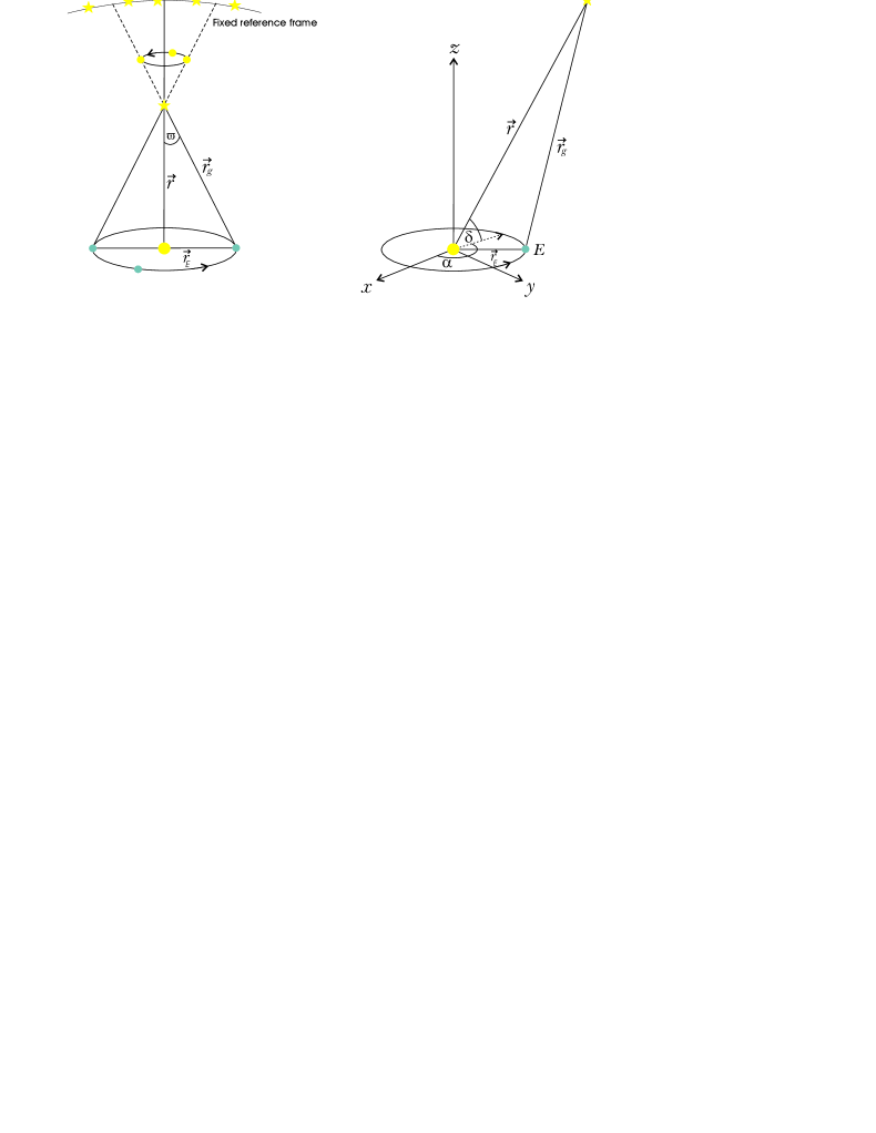
Figure 4.7: Parallax movement and correction of a star’s position

The stellar or trigonometric parallax $\varpi$ is known as the motion of a star with respect to a fixed reference system, e.g. background stars, over one year.

$$\varpi=\frac{k}{r}$$ (4.52)

with $k=\pi/648000$ and $r$, the distance of the star, expressed in astronomical units (AU) and $\varpi$ the angle between the vectors $\vec{r}_{g}$ and $\vec{r}$ in Fig. 4.7, left side. The denominator of k erases from the transformation of $\varpi$ from radians into arcseconds. More conveniently is the expression of $r$ in parsec, $1\leavevmode\nobreak\ pc=648000\rm\leavevmode\nobreak\ AU/\pi=206264.81\rm AU$. The parallax can then be written as  $\varpi=1\leavevmode\nobreak\ AU/r$ and one parsec corresponds to the distance under which an 1 AU displacement is seen as a $1\hbox{${}^{\prime\prime}$}$ angle. The apparent geocentric motion of the star is an ellipse with its semi-major axis equal to the parallax if in a first approximation the Earth orbit is described as an ellipse with its semi-major equal to one AU. As one can see, the parallax decreases with the distance of the source. The approximation $\tan{\varpi}\approx\varpi$ made here is good to about $2\cdot 10^{-17}\text{radians}\approx 10^{-7}\text{mas}$, so in practice it can be used for all parallax applications.

The diurnal parallax effect is smaller than the annual one by a factor equal to the ratio of Earth’s radius $(R_{E}=6378\rm km)$ and the astronomical unit $(1\leavevmode\nobreak\ AU=1.496\cdot 10^{8}\rm km)$. For the parallax motion of my target star (71.56 mas) this would mean a correction of $3\mu as$, which is well below the aimed precision in the measurements, so we can use the geocentric coordinates for our parallax correction.

To correct for all motion effects at once, one should use precise Earth ephemerides, giving the exact position of the Earth, $\vec{r}=\big{(}x_{E}(t),y_{E}(t),z_{E}(t)\big{)}$ in the above defined system of unit vectors (Equ. 4.49), at the time $t$ of observation with respect to the barycenter of the Solar system. The movement of the Earth should never be approximated as a circle. The position of a star in barycentric, $\vec{r}$, and geocentric, $\vec{r}_{g}$, coordinates is given by:

$$\vec{r} =r\hskip 5.69046pt\begin{cases}\cos{\delta}\cos{\alpha}&\hskip 128.0374pt\scriptstyle\alpha:\leavevmode\nobreak\ \rm right\leavevmode\nobreak\ ascention\\ \cos{\delta}\sin{\alpha}&\hskip 128.0374pt\scriptstyle\delta:\leavevmode\nobreak\ \rm declination\\ \sin{\delta}&\hskip 128.0374pt\scriptstyle r:\leavevmode\nobreak\ \rm distance\end{cases}$$

$$\vspace{1.0cm}\vec{r}_{g} =r_{g}\begin{cases}\cos{\delta_{g}}\cos{\alpha_{g}}\\ \sin{\alpha_{g}}\cos{\delta_{g}}&\hskip 119.50148pt\scriptstyle\rm g:\leavevmode\nobreak\ geocentric\\ \sin{\delta_{g}}\end{cases}$$

From Fig. 4.7 one can see that

$$\vec{r}=\vec{r}_{g}+\vec{r}_{E}$$ (4.53)

With the approximation of $r\approx r_{g}$ and $r=1/\varpi$ and plugging this into Equ. 4.53 one obtains:

$$\cos{\delta}\cos{\alpha} =\cos{\delta_{g}}\cos{\alpha_{g}}+x_{E}\varpi$$ (4.54a)

$$\cos{\delta}\sin{\alpha} =\cos{\delta_{g}}\sin{\alpha_{g}}+y_{E}\varpi$$ (4.54b)

$$\sin{\delta} =\sin{\delta_{g}}+z_{E}\varpi$$ (4.54c)

Introducing the parallactic corrections, $\Delta\alpha$ and $\Delta\delta$, which need to be added to the geocentric coordinates to derive the barycentric coordinates $(\alpha,\delta)$ we have:

$$\alpha =\alpha_{g}+\Delta\alpha \Leftrightarrow \Delta\alpha =p_{\alpha}\varpi$$ (4.55a)

$$\delta =\delta_{g}+\Delta\delta \Leftrightarrow \Delta\delta =p_{\delta}\varpi$$ (4.55b)

with $p_{\alpha},p_{\delta}$ called the parallax factors. These factors define the shape of the parallax ellipse, depending on the position on sky and $\varpi$ defines the size of this ellipse. To derive them one has to do some transformations and small angle approximations to Equations 4.54 which yield

$$\Delta\alpha =\frac{y_{E}\varpi\cos{\alpha}-x_{E}\varpi\sin{\alpha}}{\cos{\delta_{g}}}$$ (4.56)

$$\Delta\delta =-(x_{E}\varpi\cos{\alpha}+y_{E}\varpi\sin{\alpha})\sin{\delta}+z_{E}\varpi\cos{\delta}$$

Comparison with Equations. 4.55a and 4.55b yield for the parallax factors the relation:

$$p_{\alpha} =\frac{y_{E}\cos{\alpha}-x_{E}\sin{\alpha}}{\cos{\delta_{g}}}$$ (4.57a)

$$p_{\delta} =-(x_{E}\cos{\alpha}-y_{E}\sin{\alpha})\sin{\delta}+z_{E}\cos{\delta}$$ (4.57b)

The parallax factors change, depending on where on the Earth orbit the observation was taken. One can see this in the dependency of $p_{\alpha}$ and $p_{\delta}$ on $x_{E},y_{E},z_{E}$.

As one notices, to calculate the parallax factors one needs the coordinates one wants to compute. So an iterative approach is necessary, but in practice the difference between the geocentric and barycentric coordinates is mostly negligible for the computation of the parallax factors and one iteration is sufficient.

If one only corrects for the parallax, the position $(\alpha,\delta)$ of a star at epoch T is given by:

$$\alpha =\alpha_{0}+p_{\alpha}\varpi$$

$$\delta =\delta_{0}+p_{\delta}\varpi$$ (4.58)

where $\alpha_{0},\delta_{0}$ are the coordinates of the star at some reference epoch $T_{0}$.

As we will fit the parallax motion in our orbit fit we need the parallax factors, which we can compute with our measured geocentric coordinates for each epoch. We then have to fit only the size of the parallax, $\varpi$. A detailed description of the orbit fit will be given in Sec. 5.3.

4.3.11 Proper Motion

Each star has its own proper motion $\mu$, leading to a displacement on the celestial sphere when observed at an epoch $T$ compared with an observation at epoch $T_{0}$. This displacement can be in any direction. A few stars have a high proper motion of the order of $1\hbox{${}^{\prime\prime}$}/$ per year or more, but mostly the annual movement is only a small fraction of that. A star’s proper motion depends on its space motion relative to the center of the celestial sphere, the barycenter, but also on its distance. So in general the further away a star with a given space velocity, the smaller its proper motion. The velocity of a star, resulting in its proper motion is assumed to be uniform. The path of the star is then an arc of a great circle on the celestial sphere.
Ideally, proper motion is measured by comparing the position of a star in observations many years apart. The longer the baseline, the more accurate the proper motion can be derived. But the positions measured are only relative to the other stars observed with the target star and one has to assume that their positions and proper motions are known for each epoch. The best solution is to measure the positions relative to a fixed reference frame. Most satisfying would be to use objects outside our Milky Way as reference, such as other galaxies or quasars (QSO = Quasi-Stellar Object). QSO are preferable as they are more point like and many of them are also radio sources, whose position can be measured to a very high accuracy with radio interferometry. They are galactic nuclei at enormous distances and are therefore unaffected by any galactic motion.

Taking equatorial coordinates the proper motion in right ascension and declination is the time derivative of the coordinates at epoch $T_{0}$

$$\mu_{\alpha} =\left(\frac{d\alpha}{dt}\right)_{T=T_{0}}$$

$$\mu_{\delta} =\left(\frac{d\delta}{dt}\right)_{T=T_{0}}$$ (4.59)

$\mu_{\delta}$ corresponds to a full (great circle) angle on the sky, but $\mu_{\alpha}$ is reckoned on the equator. Its actual component along the local small circle is given by $\mu_{\alpha}\cos{\delta}$. $\mu_{\alpha}$ and $\mu_{\delta}$ are normally expressed in arcseconds per year, however if $\mu_{\alpha}$ is given in seconds of time per year, one has to multiply it by a factor of 15 to get arcseconds.
A star’s motion can be separated into a radial motion $V_{r}$ (see Sec. 4.3.8) and a transverse motion on a tangent plane to the celestial sphere. The transverse motion equals the proper motion $\mu=\sqrt{\mu_{\alpha}^{2}\cos^{2}{\delta}+\mu_{\delta}^{2}}$. With $\phi$ being the position angle of this motion measured from North over East, the components of the proper motion in right ascension and declination can be written as:

$$\mu_{\alpha}\cos{\delta} =\mu\sin{\phi}$$

$$\mu_{\delta} =\mu\cos{\phi}$$ (4.60)

One can now calculate a star’s position for any given epoch, if one only assumes proper motion and parallactic motion. The position $(\alpha,\delta)$ of a star at epoch T is then given by:

$$\alpha =\alpha_{0}+(T-T_{0})\mu_{\alpha}^{*}+p_{\alpha}\varpi$$

$$\delta =\delta_{0}+(T-T_{0})\mu_{\delta}+p_{\delta}\varpi$$ (4.61)

with $\mu_{\alpha}^{*}$ being short for $\mu_{\alpha}\cos{\delta}$.

Secular Acceleration

The secular acceleration is a variation in the proper motion and is a purely geometric effect, due to an object which is approaching or receding. Writing the proper motion as a function of the object’s space velocity $V$, its angle $\Theta$ with the direction barycenter-star and its distance $r$

$$\mu=\frac{V\sin{\Theta}}{r}$$ (4.62)

and calculating its derivative with respect to time $t$, one gets:

$$\frac{d\mu}{dt}=-\frac{V}{r^{2}}\sin{\Theta}\frac{dr}{dt}+\frac{V}{r}\cos{\Theta}\frac{d\Theta}{dt}$$ (4.63)

With $\frac{d\Theta}{dt}=-\mu$ and $V\cos{\Theta}=V_{r}=\frac{dr}{dt}$ and using Equ. 4.62 one can write

$$\frac{d\mu}{dt}=-\frac{2\mu}{r}V_{r}$$ (4.64)

Expressing $\mu$ in arcseconds per year , the distance $\varpi=\frac{1}{r}$ in arcseconds and $V_{r}$ in km/s, the secular acceleration can be calculated by:

$$\frac{d\mu}{dt}=-2.05\cdot 10^{-6}\mu\varpi V_{r}$$ (4.65)

Using the values for proper motion ($\mu=1.5\hbox{${}^{\prime\prime}$}$/year) and parallax ($\varpi=71.56\rm\leavevmode\nobreak\ mas$) from the HIPPARCOS catalog and a radial velocity $V_{r}=63\rm\leavevmode\nobreak\ km/s$ for our target star, the secular acceleration amounts to $-13.84\cdot 10^{-6}\rm\leavevmode\nobreak\ arcsec\leavevmode\nobreak\ yr^{-1}$. This would result in a change in proper motion of 0.02 mas/yr over the 1.5 yrs time baseline of our observations, which we will not be able to measure. We can therefore stay with the truncation of the Taylor series of the star’s motion after the first term and assume the proper motion of our target as constant in time. As the reference star is much further away and its proper motion therefore is way smaller, the effect for it will be even smaller.

4.4 Plate-scale and Detector Rotation Stability

Doing astrometry with NACO, one has to take care of two effects. The global pixel- or plate-scale can change and field distortions can be present, both effects can change with time. To monitor and correct the possible change of pixel-scale and also the rotation of the detector, I observed a reference field in the globular cluster 47 Tuc every time right before the target field. To minimize these effects, I centered the stars on the same pixel positions at the beginning of each observation in both, the target and reference field, and executed the same jitter pattern each time. As long as the jitter pattern is the same in each observation, I do not have to take care about the absolute distortions, but have to monitor, if they change with time. Experience from other observers using NACO, indicates that the distortion pattern is stable over time. If the distortions are constant with time, they should be the same for each observation, and only the change in pixel-scale has to be corrected. Unfortunately, it is not so easy to separate the change in the globular pixel-scale and the field distortions, which create different local pixel-scales. Also, the final image, on which I work, is the sum of the shifted and added single images. The distortions, present in each single image, are smeared out in the final image, making it very difficult to model them, as they are dependent on the size and distribution of the jitter offsets. NACO is at the Nasmyth focus, but it does not have an optical de-rotator. It rotates as a whole instrument, instead. Therefore variable flexures exist in this Nasmyth instrument and the distortions from the reference field can probably not be used to correct the target field.
The only thing left is to model a global pixel-scale, assuming it only changes on a global scale and has no direct cross-talk with the distortions.

To calculate the changes between the different epochs, I chose the same 11 stars for each epoch in the observed reference field. In Fig. 4.8 the stars used for the distortion fit are marked.

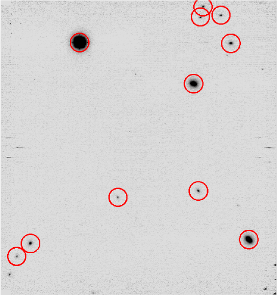
Figure 4.8: Stars in the reference field in 47 Tuc used to calculate the change in pixel-scale and rotation between the different epochs.

As I do not need to measure an absolute plate-scale or rotation of the detector, but only relative values, I chose epoch 9 as the reference epoch to which all other epochs are mapped. This epoch was chosen, because it is the middle one in time of all observations. I then mapped the positions of the stars in each epoch to the positions measured in epoch 9 with a linear coordinate transformation, calculating a shift in $x$ and $y$, scale in $x$ and $y$, and a rotation and skew. The skew is realized by allowing a different rotation for the $x$ and $y$ axes. The parameters were calculated with the geomap program, which is part of the IRAF reduction and data analysis software.

The calculated values for each epoch are shown in Fig. 4.9

Figure 4.9: Calculated distortion parameters of all epochs. The parameters for shift, scale and rotation in $x$ and $y$, respectively, are shown from top to bottom versus the MJD of the observation. For the scale and rotation parameters the mean value and the standard deviation are given, for an impression of the stability of these parameters over time.

The panels show from top to bottom the calculated shift, scale and rotation for the $x$ and $y$ direction versus the Modified Julian Date (MJD), for each epoch mapped to epoch 9. The much larger values for the shift of the first epoch are due to a rotation of the frame about 90^∘, due to an error in the value of the applied rotation of the detector. I corrected the coordinates of the stars to this rotation, but their positions on the frames nevertheless differ by roughly +75 pixel on the $x$-axis and -100 pixel on the $y$-axis. But the shift is not the important parameter, as it does not change the distance between the stars. The more interesting values are the scale and rotation. Here the mean value and the standard deviation are also given in the respective panels. The standard deviation gives an impression of the stability of the parameters over time. It seems the larger the separation in time is for the first nine epochs, the more different is the plate-scale, but this would have to be explored in more detail with more data doing a distortion analysis for NACO. The calculated rotation between the different epochs does not show a trend with time. For the 47 Tuc observations, the detector was rotated by $42\hbox{${}^{\circ}$}$ anticlockwise. The scatter of the measured rotation between the epochs gives the accuracy with which the applied rotation of the detector can be performed. The scatter is quite large, 0.26 - 0.27 degree, but there is no large difference for the two axes, indicating only a very small skew. Because the detector is again rotated between the observations of the reference and the target field, and I cannot assume that the rotation error is the same for both fields in the same night, I cannot correct for the rotation between the epochs. As there are only two stars in the target field, an independent estimate of the differential rotation between the epochs for this field is not possible. I added the scatter of the rotation parameter over time, measured as a mean of the $x$- and $y$-rotation, in the reference field as the uncertainty of the later calculated position angle between the two stars in the target field.

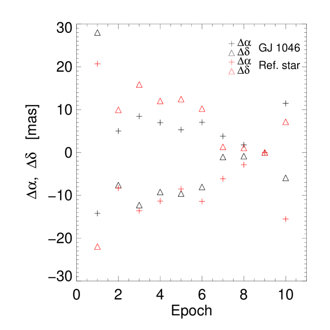
Figure 4.10: Relative change in positions due to the plate-scale correction. Shown are the values for $\Delta\leavevmode\nobreak\ \alpha=\alpha-\alpha_{corr}$ and $\Delta\leavevmode\nobreak\ \delta=\delta-\delta_{corr}$ for both stars in the target field. The opposite directions of the changes for GJ 1046 and the reference star are expected, due to the fact the the coordinates are calculated from the reference point, which is almost in the middle of the detector. The large displacement i n epoch 1 is due to the larger change in pixel-scale compared with the other epochs. The visible trends correspond to ones already visible in Fig. 4.9.

4.4.1 Plate-scale Correction

The detector distortions are the last effect changing the true positions of the stars. Therefore one should correct for them first. I assumed that the change in pixel-scale at any epoch with respect to the one in epoch 9 is the same in the reference field and the target field. To correct for the change in pixel-scale I multiplied the FITS header keywords CDi_j$=s_{i}m_{ij}$ (Equ. 4.4) with the scale factors derived from the distortion fit:

$$\rm new\leavevmode\nobreak\ CD_{11} =\rm CD_{11}*\text{x-scale}$$ (4.66)

$$\rm new\leavevmode\nobreak\ CD_{12} =\rm CD_{12}*\text{x-scale}$$

$$\rm new\leavevmode\nobreak\ CD_{21} =\rm CD_{21}*\text{y-scale}$$

$$\rm new\leavevmode\nobreak\ CD_{22} =\rm CD_{22}*\text{y-scale}$$

This was done for every epoch (for the first epoch the $x$- and $y$-scale are exchanged due to the 90^∘ rotation) and following this, the measured pixel coordinates of the stars were transformed to celestial coordinates, as described in Chap. 4.2.3, using the new plate-scale. After that, the corrections for differential refraction and aberration were calculated and applied again (Chap. 4.3.3 and 4.3.6). That the celestial positions changed indeed due to the plate-scale correction can be seen in Fig. 4.10 where the change, after the transformation from $x/y$ coordinates to celestial coordinates, in right ascension and declination is plotted in milli-arcseconds for each epoch.
A scaling of the image itself before measuring the positions would involve interpolation, which again can introduce errors. I therefore chose the applied way of correction, because here I do not have to work on the images directly to change the pixel-scale. I therefore corrected directly the coordinates of the stars, which is more precise. The RMS given by the fit for the coordinate mapping takes all transformations into account. I cannot use this value as an estimate for the plate-scale correction alone, as it also takes for example the rotation into account. To estimate the precision of the plate-scale correction I took star pairs in the reference field in one epoch and calculated their separation. Taking the separation of the same star pairs in epoch 9, the reference epoch, as the separation with a plate-scale of the theoretical value of 27.15 mas/px, I could calculate the pixel-scale of the other epochs by comparing the separations:

$$\text{plate-scale\_i}=\frac{\text{separation\_epoch\_9}}{\text{separation\_epoch\_i}}*27.15\leavevmode\nobreak\ \frac{mas}{pixel}$$ (4.67)

I did this for 100 random star pairs for each epoch to have good statistics. The standard deviation of the distribution of pixel-scales calculated this way is then taken as the uncertainty in the pixel-scale correction for the later separation measurement of the two stars. In Tab. 4.3 the uncertainties in the pixel-scale are listed for each epoch.

Epoch	pixel-scale	pixel-scale
	uncertainty [$\frac{mas}{px}$]	uncertainty [%]
1	0.046	0.171
2	0.035	0.127
3	0.027	0.100
4	0.018	0.066
5	0.016	0.058
6	0.045	0.164
7	0.014	0.051
8	0.032	0.117
9	0.000	0.000
10	0.029	0.105

Table 4.3: Uncertainties in the pixel-scale. Calculated by randomly taking 100 star pairs in the reference field, calculating the changed pixel-scale relative to epoch 9, and taking the standard deviation of the distribution of derived pixel-scales as uncertainty.

These first results in this chapter show, that in multi-epoch astrometry the most challenging task is to measure and correct the pixel-scale very precisely to obtain milli- or even micro-arcsec astrometric solutions.

Chapter 5 The Orbit Fit

5.1 Preparing the Coordinates for the Orbital Fit

To fit an orbit to the positions of the two stars derived so far, one needs to apply some last transformations and calculations. In a first approach I re-transformed the celestial coordinates of the target star GJ 1046 and the reference star 2MASS 02190953 -3646596 to pixel coordinates with the IDL routine adxy.pro from the IDL astrolib. This routine is the inverse of xyad.pro, which I used to transform pixel coordinates into celestial coordinates in Chap. 4.2.3. I then finally corrected the coordinates for the nominal rotation of 6^∘ of the detector, relative to the North direction. The $x$ and right ascension axes, as well as the $y$ and declination axes are now parallel. One can now work with the separations of the two stars in $x$ and $y$ and their change with time.
Additionally, I calculated the separation and position angle of the two stars. Because of the large separation of the stars, one cannot just calculate the separation in Cartesian coordinates. One has to calculate the separation $\rho$ of the two stars along a great circle using the cosine formula (Green, 1985, p. 12):

$$\rho=\cos^{-1}{\left(\sin{\delta_{1}}\sin{\delta_{2}}+\cos{\delta_{1}}\cos{\delta_{2}}\cos{\Delta\alpha}\right)}$$ (5.1)

Where $\delta_{1}$ and $\delta_{2}$ are the declination of the two stars, star 1 = reference star and star 2 = GJ 1046, and $\Delta\alpha$ is the difference in their right ascension.
The position angle $\Theta$ of GJ 1046 relative to the reference star, measured from North through East from the Meridian containing the reference star is calculated using the four-parts formula (Green, 1985, p. 12):

$$\Theta=\tan^{-1}{\left(\frac{\sin{\Delta\alpha}}{\cos{\delta_{1}}\tan{\delta_{2}}-\sin{\delta_{1}}\cos{\Delta\alpha}}\right)}$$ (5.2)

The errors of the separation and position angle, resulting from the positional uncertainties of the stars, are between 0.22 - 1.45 mas for the separation and between 0.00045^∘- 0.00252^∘ for the position angle. However, a much larger uncertainty due to the pixel-scale variability and the detector rotation uncertainty had to be added for each epoch. The resulting uncertainties in the separation are between 15.30 mas and 50.90 mas and 0.26072^∘ in the position angle with only very small differences for the single epochs. A summary of the calculated separation and position angle values together with their errors is given in Tab. 5.1 for each epoch. In column two the separation and position angle are noted, column three lists the combined errors due to the position measurement and the correction for differential refraction and aberration. In column four the error due to the pixel-scale uncertainty and the detector rotation are given and column five finally lists the combined errors of all these effects.

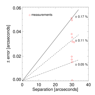
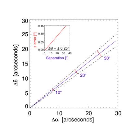
Figure 5.1: Effect of separation between the target and reference star on the precision obtainable for the separation (left panel) and the position angle (right panel). For more details and explanation see text.

This already shows, how crucial it is to measure the pixel-scale and the rotation of the detector very accurately. The large separation of the target and reference star yields this large separation and position angle uncertainty. In Fig. 5.1 the effect of the separation between the target and reference star on the obtainable precision is shown. The left panel shows the error in the separation in arcseconds as a function of pixel-scale uncertainty and separation. The lines represent the errors in the separation between the stars for three different values of uncertainty ($\pm 0.05\%,\leavevmode\nobreak\ \pm 0.11\%,\leavevmode\nobreak\ \pm 0.17\%$) in the pixel-scale. The red diamonds represent my measured uncertainties. The right panel shows the error in the separation in right ascension ($\Delta\alpha$) and declination ($\Delta\delta$) due to the uncertainty in the position angle. Shown is the case for a position angle of 42^∘ (solid line) with an uncertainty of $\pm 2.5\hbox{${}^{\circ}$}$ (dashed lines). This 10 times larger error than measured was taken for reasons of better depiction of the effect. The separation between the stars is indicated along the lines by marks at 10^′′, 20^′′ and 30^′′. Projecting the error onto the directions of right ascension and declination leads to large errors in these two values. In the small inlet the size of the uncertainty of the position angle, $\Theta\pm 0.25\hbox{${}^{\circ}$}$ (red in the big panel), along the direction perpendicular to the separation (blue in the big panel) is shown in seconds of arc as function of the separation.

			Pos., Refrac., Aberr.		pixel-scale, de-rotator		$\sqrt{\sum_{\scriptstyle i}\Delta\rho_{i}^{2}}$	$\sqrt{\sum_{\scriptstyle i}\Delta\Theta_{i}^{2}}$
Epoch	$\rho\leavevmode\nobreak\ [\hbox{${}^{\prime\prime}$}]$	$\Theta\leavevmode\nobreak\ [\hbox{${}^{\circ}$}]$	$\Delta\rho_{1}$ [mas]	$\Delta\Theta_{1}\leavevmode\nobreak\ [\hbox{${}^{\circ}$}]$	$\Delta\rho_{2}$ [mas]	$\Delta\Theta_{2}\leavevmode\nobreak\ [\hbox{${}^{\circ}$}]$	[mas]	[∘]
1	29.7709	37.96	0.23	$4.4\cdot 10^{-4}$	50.91	0.26	50.90	0.26
2	29.8758	38.54	0.54	$9.9\cdot 10^{-4}$	37.94	0.26	38.04	0.26
3	29.9273	38.57	1.06	$19.0\cdot 10^{-4}$	29.93	0.26	29.98	0.26
4	29.9330	38.62	0.28	$5.0\cdot 10^{-4}$	19.76	0.26	19.70	0.26
5	30.0251	38.78	0.40	$7.5\cdot 10^{-4}$	17.41	0.26	17.43	0.26
6	30.1134	38.38	0.47	$8.6\cdot 10^{-4}$	49.39	0.26	49.42	0.26
7	30.1570	38.54	0.33	$6.1\cdot 10^{-4}$	15.38	0.26	15.32	0.26
8	30.2174	38.47	0.36	$6.7\cdot 10^{-4}$	35.35	0.26	35.42	0.26
9	30.2864	38.53	0.40	$7.1\cdot 10^{-4}$	0.00	0.26	0.40	0.26
10	31.3265	38.62	1.45	$25.2\cdot 10^{-4}$	32.89	0.26	33.00	0.26

Table 5.1: Summary of the measured separation $\rho$ and position angle $\Theta$ together with their uncertainties. The third column list the combined errors due to the PSF fit and the correction for differential refraction and aberration. In column four the errors due to the pixel-scale uncertainty and the detector rotation are given and column five finally lists the combined errors of all these effects.

5.2 Theory of Deriving the Orbital Elements

The orbit of a planet around its host star, as well as the motion of the star due to a companion, are ellipses with the common center of mass of the two bodies at one of the focal points of both ellipses. To describe the orbital motion of the companion or the host star, one needs to know where the body is at any time $t$. The orbital elements are the same for the two bodies, except the size of the semi-major axis. To derive the orbital elements one can regard the ellipse as a projection of a circle. In Fig. 5.2 the principal components of such an ellipse are depicted.

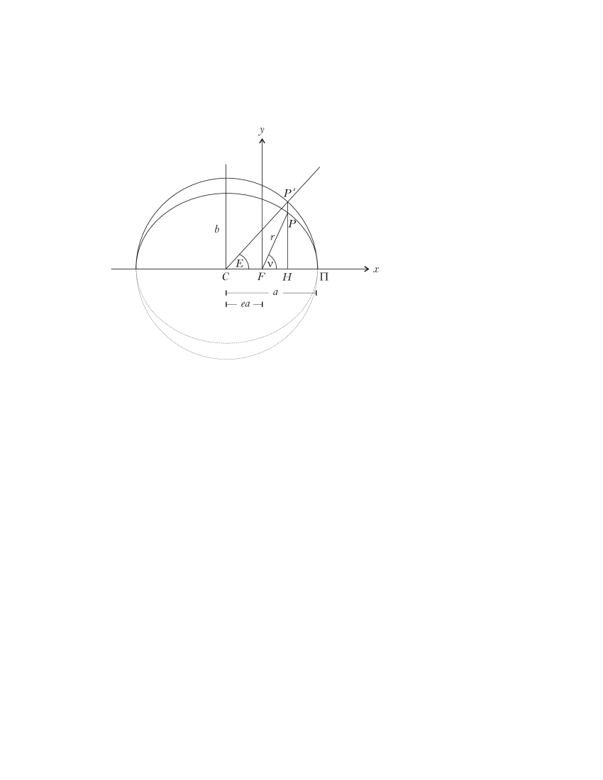
Figure 5.2: Principle elements of an ellipse with the definition of the eccentric anomaly $E$ and the true anomaly $\nu$.

The denotation is as follows:
$C$ center of the ellipse $F$ focal point of the ellipse $\Pi$ periastron $a$ semi-major axis $b$ semi-minor axis $e$ eccentricity $ea$ distance from $C$ to $F$ $P$ point on ellipse at time $t$ $P^{{}^{\prime}}$ point on circle which is projected onto the ellipse $r$ radius vector $E$ eccentric anomaly $\nu$ true anomaly

The eccentric anomaly $E$ is defined as the angle between the semi-major axis $a$ and the direction from the center of the ellipse to the point $P^{{}^{\prime}}$ on the circle. It is zero at the periastron $\Pi$ and increases by $2\pi$ during one orbit. The true anomaly is the angle between the distance $\overline{F\Pi}=a-ae=a(1-e)$ and the distance $\overline{FP}=r$, which is the radius vector at time $t$. Looking at Fig. 5.2, one can see that for a Cartesian coordinate system with its origin at $F$, the $x$ and $y$ values of the point $P$ in polar coordinates in the plane of the orbit are given by:

$$X=r\cos{\nu} =a(\cos{E}-e)$$

$$Y=r\sin{\nu} =a\sqrt{1-e^{2}}\sin{E}$$ (5.3)

and the distance of $P$ from the focal point $F$ is:

$$r=a(1-e\cos{E})=\frac{a(1-e^{2})}{1+e\cos{\nu}}$$ (5.4)

Defining the mean anomaly $M$ at time $T$ by the mean motion $n=\frac{2\pi}{P}$, with $P$ being the period and $T_{p}$ the time of periastron:

$$M=n(T-T_{p})=E-e\sin{E}$$ (5.5)

one can calculate the eccentric anomaly $E$ at any time using an iterative approach. The last expression $M=E-e\sin{E}$ is known as Kepler’s equation. Once $E$ is determined one can compute $r$ and $\nu$ from Equ. 5.4 and from:

$$\tan{\frac{\nu}{2}}=\sqrt{\frac{1+e}{1-e}}\tan{\frac{E}{2}}$$ (5.6)

In the simple case of visual binaries, one centers the primary in the local coordinate system to describe the orbital motion of the companion with respect to the primary star, but the equations are also true for the motion of the primary around the secondary. The coordinates of the companion on the tangential plane on the sky with respect to the primary, expressed in seconds of arc, are then defined by the separation $\rho$ and the position angle $\theta$, starting from North on eastward:

$$x=\rho\sin{\theta}$$

$$y=\rho\cos{\theta}$$ (5.7)

5.2.1 The Thiele-Innes Constants

Each observation of a visual binary yields a pair of coordinates at a given time $T$. These coordinates are the separation of the two stars and the position angle. After a hopefully sufficiently long time interval of observations one has a series of values ($\rho,\theta,T$) or equivalently $(x,y,T)$. These measured values give the apparent orbit in the $x/y$ plane on the sky.
The true orbit of the companion about the primary, which one wants to obtain, is an ellipse with the primary situated at one focus $F$. Projecting this ellipse onto the plane of the sky yields again an ellipse, the apparent orbit. This apparent ellipse is not a Keplerian ellipse anymore. The focus $F$ of the true ellipse doe not coincident with a focus of the apparent ellipse, meaning the primary is not seen at a focus. The semi-major axis of the apparent orbit does not correspond to the semi-major axis of the true orbit either and therefore does not lie along the projection of the diameter that contains the periastron $\Pi$. Only the projection of the center of the true orbit appears at the center of the apparent orbit and the areas on the apparent ellipse are projections of the areas of the true ellipse. Kepler’s $2^{nd}$ law of proportionality of the areas swept by the radius vector still holds.

With the orbital parameters defined in Chap. 1.1 one can transform the local apparent coordinates $(\rho\sin{\Theta},\leavevmode\nobreak\ \rho\cos{\Theta})$ in the coordinate system $OXY$ to the true coordinates in the coordinate system $Oxy$. With the scale of the true orbit in arcseconds, $a\hbox{${}^{\prime\prime}$}=a\varpi$ with the parallax $\varpi$ and the semi-major axis $a$, one can write the true coordinates in the plane of the orbit, also expressed in arcseconds, as

$$\mathbf{B}\begin{cases}X=\varpi r\cos{\nu}\\ Y=\varpi r\sin{\nu}\end{cases}$$

To transform $\mathbf{B}$ into $\mathbf{r}=(\rho\sin{\theta},\rho\cos{\theta})$ one has to perform three transformations.
The first one is a rotation by $-\omega$ around the $Z$-axis which is perpendicular to the $X/Y$-plane, the true orbital plane. After this, one has to account for the projection angle $i$, the inclination, between the true orbital plane and the plane perpendicular to the line of sight. The intermediate coordinates can be written as:

$$X_{inter} =X\cos{\omega}-Y\sin{\omega}$$

$$Y_{inter} =\cos{i}(X\sin{\omega}-Y\cos{\omega})$$ (5.8)

One then has to rotate these coordinates by $-\Omega$ around the z-axis, which is in the direction of the line of sight and perpendicular to the tangential plane. Finally a permutation of the abscissa and ordinate needs to be performed to obtain the coordinate system $Oxy$ in the tangential plane

$$x =X_{inter}\sin{\Omega}+Y_{inter}\cos{\Omega}$$

$$y =X_{inter}\cos{\Omega}+Y_{inter}\sin{\Omega}$$

Combining this with Equ. 5.8 one finally can write the apparent coordinates expressed by the true coordinates as:

$$x= X(\cos{\omega}\sin{\Omega}+\sin{\omega}\cos{\Omega}\cos{i})$$

$$+Y(-\sin{\omega}\sin{\Omega}+\cos{\omega}\cos{\Omega}\cos{i})$$

$$y= X(\cos{\omega}\cos{\Omega}-\sin{\omega}\sin{\Omega}\cos{i})$$

$$+Y(-\sin{\omega}\cos{\Omega}-\cos{\omega}\sin{\Omega}\cos{i})$$

With the Thiele-Innes constants defined as:

$$X_{TI1} =a(\cos{\omega}\sin{\Omega}+\sin{\omega}\cos{\Omega}\cos{i})$$

$$Y_{TI1} =a(-\sin{\omega}\sin{\Omega}+\cos{\omega}\cos{\Omega}\cos{i})$$

$$X_{TI2} =a(\cos{\omega}\cos{\Omega}-\sin{\omega}\sin{\Omega}\cos{i})$$

$$Y_{TI2} =a(-\sin{\omega}\cos{\Omega}-\cos{\omega}\sin{\Omega}\cos{i})$$ (5.9)

one can write in short form:

$$x =\frac{r}{a}\cos{\nu}X_{TI1}+\frac{r}{a}\sin{\nu}X_{TI2}$$

$$y =\frac{r}{a}\cos{\nu}Y_{TI1}+\frac{r}{a}\sin{\nu}Y_{TI2}$$ (5.10)

5.3 The Astrometric Orbit Fit

In the context of this work, I do not measure the companion’s motion around the star directly, but instead the star’s motion about the common center of mass of the system. Therefore the orbital motion ($x_{orbit},y_{orbit}$) I see, is related to the star’s motion and semi-major axis. $x_{orbit}$ and $y_{orbit}$ are the expressions derived in Equ. 5.10 with an index $orbit$ added to point out that this is the orbital motion of the star due to the companion in the following equations.

In my case I already have some of the orbital elements from the radial velocity measurements. These are: the Period $P$, the eccentricity $e$, the longitude of periastron $\omega$ and the time of periastron $T_{p}$. The semi-major axis $a$ is related to the inclination $i$ over Equ. 1.4, so the only two orbital parameters one has to solve for, after fixing the spectroscopic parameters, are the inclination of the orbit and the longitude of the ascending node $\Omega$. These two angles of the orbit of the star are the same for the companion. I could fix the values of $P,\leavevmode\nobreak\ e,\leavevmode\nobreak\ \omega,\rm\leavevmode\nobreak\ andT_{p}$ to the values derived in the spectroscopic orbit fit, because the accuracy from this fit is much higher than the accuracy with which they could be derived in the astrometric fit.

One can write the position of the star on the sky depending on proper motion and parallax of the center of mass and the reflex motion of the star at any time $T$ as:

$$\alpha =\alpha_{0}+(T-T_{0})\mu_{\alpha}+p_{\alpha}\varpi+x_{orbit}$$

$$\delta =\delta_{0}+(T-T_{0})\mu_{\delta}+p_{\delta}\varpi+y_{orbit}$$ (5.11)

where $\alpha_{0},\leavevmode\nobreak\ \delta_{0}$ are the position of the star at epoch $T_{0}$, $\mu_{\alpha}$ and $\mu_{\delta}$ are the proper motion and $p_{\alpha},\leavevmode\nobreak\ p_{\delta}$ are the parallax factors in right ascension and declination, respectively. As I measure relative positions and not absolute ones, the positions $\alpha_{0},\leavevmode\nobreak\ \delta_{0}$ are replaced by the separation of the two stars in right ascension and declination $\Delta\alpha_{0},\leavevmode\nobreak\ \Delta\delta_{0}$ and $\alpha,\leavevmode\nobreak\ \delta$ then correspond to separations, too.

To solve this equation one also has to fit for the proper motion and parallax of the target star relative to the reference star. As seen in the previous sections, the uncertainty in the pixel-scale and the orientation of the detector lead to large errors in the final separation and position angle, with the error in the separation being still a lot smaller than that of the position angle. The orbital period of the companion of GJ 1046, and therefore of GJ 1046 itself, is 169 days, almost half a year. Special care has to be taken to disentangle the orbital motion from the parallax motion. For this, the observations were timed in such a way that measurements over almost a full orbit were obtained. In Fig. 5.3 an example of a simulated astrometric signal of GJ 1046 with proper motion, parallax and orbital motion is shown as a change in right ascension and declination over one year. The HIPPARCOS proper motion and parallax are taken and $i=45\hbox{${}^{\circ}$}$ and $\Omega=60\hbox{${}^{\circ}$}$ are assumed. As the proper motion of GJ 1046 is very high, it totally dominates its motion and pulls the parallax + orbital ellipse apart into a wave-like motion (left panel). Subtracting the proper motion in the simulation, one can see the orbital motion due to the companion, but still dominated by the parallax (middle panel). The curve is not a perfect ellipse as in the case of pure parallax motion and is not closing after one full orbit of the Earth around the sun. Finally the pure orbital motion without parallax and proper motion is displayed (right panel). As one can see, it is very important to know/measure the parallax motion to distinguish the orbital motion from it. Note the different scales in the changes of right ascension and declination in the three different cases.

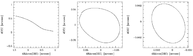
Figure 5.3: Simulated change in declination versus right ascension of the orbit of GJ 1046. The left panel shows a simulated astrometric signal for GJ 1046 (see text for details). The other two panels show the simulated astrometric signal without proper motion and with (middle) and without (right) parallax, respectively. Note the different scales in the changes of right ascension and declination in the three different cases.

The fit for the orbital parameters was performed by Rainer Köhler from the Landessternwarte Heidelberg, who is experienced in deriving orbital solutions, using his orbit fit program. A model is calculated based on Equations 5.11 which is then compared with the actual measurements by minimizing $\chi^{2}$, using a Levenberg-Marquardt algorithm (LMA) to (Press et al., 1992).
A first fit was performed, accounting only for the measurements of the separations of GJ 1046 from the reference star, because of the relatively smaller error of this parameter. No orbital motion was taken into account at this step, so Equations. 5.11 reduce to:

$$\alpha =\Delta\alpha_{0}+(T-T_{0})\mu_{\alpha}+p_{\alpha}\varpi$$

$$\delta =\Delta\delta_{0}+(T-T_{0})\mu_{\delta}+p_{\delta}\varpi$$ (5.12)

We took the values for the proper motion and parallax from the HIPPARCOS catalog for a first test, $\mu_{\alpha}=1394.10$ mas/yr, $\mu_{\delta}=550.05$ mas/yr, $\varpi=71.56$ mas, so the only free parameters are the separation zero-points $\Delta\alpha_{0}\rm\leavevmode\nobreak\ and\leavevmode\nobreak\ \Delta\delta_{0}$. The calculated separations from the model parameters for $\alpha$ and $\delta$ are then compared with the measured ones for each epoch.

The second approach was to include the orbital movement in the fit. This was done by scanning the possible angles for the inclination $i$ and the longitude of the ascending node $\Omega$ in one degree steps and calculating a $\chi^{2}$ value for each ($i,\Omega$) pair. Again, the only free parameters in Equ. 5.11 for the LMA were $\Delta\alpha_{0}\rm\leavevmode\nobreak\ and\leavevmode\nobreak\ \Delta\delta_{0}$, as $i$ and $\Omega$ were given at each step. For each ($i,\Omega$) pair a model was calculated for the separation $\rho$ and this time also for the position angle $\Theta$. Inclination $i$ and ascending node $\Omega$ are needed to calculate the Thiele-Innes constants (Equ. 5.9) to derive the orbital influence on the separation and position angle. After scanning $i$ from 0-180^∘ and $\Omega$ from 0-360^∘ we have a $\chi^{2}$ map for the full parameter space of these two angles. We again used the proper motion and parallax from the HIPPARCOS catalog. We can now search the resulting $\chi^{2}$ map for a minimum.

Chapter 6 Results

Due to the large uncertainties in the detector orientation and pixel-scale correction I was not able to detect any astrometric motion of the star due to its brown dwarf companion. Only a formal value for the inclination of the system and thus for the mass of the companion could be derived, but with low significance of the results, see Sect. 6.1.

Using the HIPPARCOS values for proper motion and parallax and not taking any orbital motion into account for the model fit, results in a good agreement of the model with the measured separation changes. In Fig. 6.1 the measured separation between the stars is plotted versus time. Overplotted as the solid line is the model with the motion calculated from the HIPPARCOS values for parallax and proper motion. The very good agreement indicates that the assumption of a small or negligible parallax and proper motion of the reference star was right and that we only see and detect the motion of GJ 1046 itself. The $\chi^{2}$ value of this model fit is $\chi^{2}=7.63$, with 18 degrees of freedom (DoF) the chance probability of this value is $p(\chi^{2})=0.984$. Therefore the confidence for rejecting the model without orbital motion is onlt 1.6%. In principle one should stop at this point and accept the model, which only takes proper motion and parallax movement of the star into acoount, as precise enough to represent the data. However, from the radial velocity measurements, I know about the presence of a companion, hence also a model including orbital motion is calculated and fit to the data.

Figure 6.1: Measured separation between GJ 1046 and the reference star vs. time for the 10 observed epochs. The error bars represent the uncertainty in the separation due to the pixel-scale uncertainty. Epoch 9 has only a very small error bar as it is the reference epoch for the measurement of the pixel-scale changes (see Sect. 4.4). Overplotted is the model for the separation changes calculated with the HIPPARCOS values for proper motion and parallax (solid line). No orbital motion is taken into account. The good agreement of the measurements with the model shows that the reference star has indeed only a very small intrinsic parallax and proper motion.

6.1 The Orbit

Due to the large uncertainty in the alignment of the detector a transformation of the separation onto the right ascension and declination axes results in large error bars in these two directions. An attempt to fit a model based on Equ. 5.11 with the separation at epoch zero $\Delta\alpha_{0},\leavevmode\nobreak\ \Delta\delta_{0}$, parallax $\varpi$, proper motion $\mu_{\alpha}$ and $\mu_{\delta}$, inclination $i$ and longitude of the ascending node $\Omega$ as free parameters led to resulting values of the proper motion and parallax strongly diverging from the HIPPARCOS values. Even though a small deviation is in principle possible, as only relative motions to the reference star are measured, a deviation of up to 200 mas, as derived in the fit, is not possible. Additionally, the results from the fit without orbital motion using the HIPPARCOS values showed a very good agreement with these values. Therefore, the proper motion and parallax were fixed to the HIPPARCOS values in the following approach to fit the orbital motion, as we are not able to improve these values.
In Fig. 6.2 the resulting $\chi^{2}$ contour map from the model fit with orbital motion to the measured separation and position angle is depicted. The white contour represents the $1\sigma$ (68.3%) and the black contours the $2\sigma$ (95.4%) and $3\sigma$ (99.7%) confidence levels.

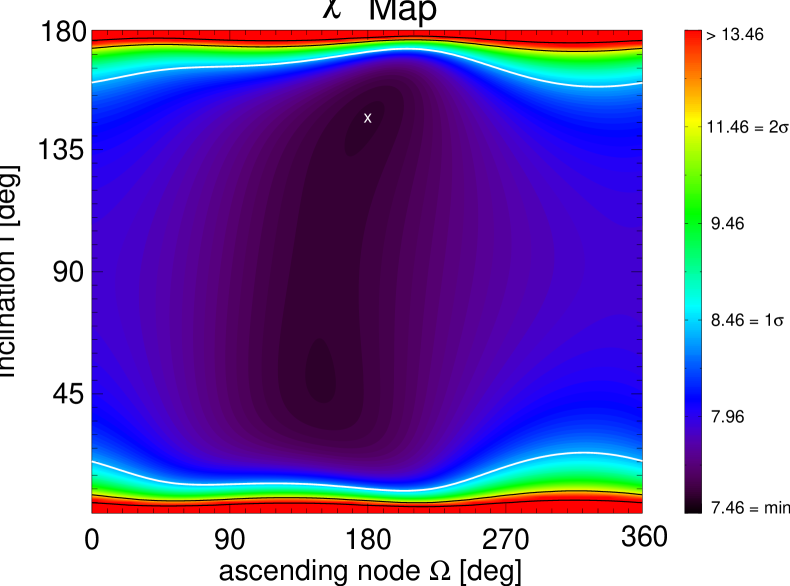
Figure 6.2: $\chi^{2}$ contour map for fitting the orbital motion to the separation and position angle measurements. The spectroscopic parameters were fixed, as well as the parallax and proper motion (HIPPARCOS values). The inclination $i$ and the ascending node $\Omega$ were looped through, leaving the zero-point separation in declination and right ascension as the only free fit parameters. The white contour represents the $1\sigma$ (68.3%) confidence level and the black contours the $2\sigma$ (95.4%) and $3\sigma$ (99.7%) confidence levels. The white cross marks the formally best fit solution found at $i=145\hbox{${}^{\circ}$}$ and $\Omega=180\hbox{${}^{\circ}$}$.

The formally best fit is achieved with an inclination $i=145.0\hbox{${}^{\circ}$}$ ($180\hbox{${}^{\circ}$}-i=35\hbox{${}^{\circ}$}$) and a longitude of the ascending node $\Omega=180\hbox{${}^{\circ}$}$, leading to a formal mass of the companion of $m_{p}=48.5\leavevmode\nobreak\ M_{Jup}$, calculated with the mass function (Equ. 1.3). This would mean that the companion is indeed a brown dwarf, residing in the brown dwarf desert. However, this result cannot be considered significant, as already the simplier model without orbital motion could not be rejected with sufficient confidence. Likewise the model including orbital motion cannot be rejected. The confidence for rejection of this model is only 3.7% (DoF = 16, $\chi^{2}=7.46$), but setting better constraints on the orbital parameters is not possible. This is also indicated by the large formal errors derived for the inclination $i$ and the ascending node $\Omega$. Already within $1\sigma$, inclinations from $8.5\hbox{${}^{\circ}$}-170.5\hbox{${}^{\circ}$}$ are possible. The $1\sigma,\leavevmode\nobreak\ 2\sigma$ and $3\sigma$ levels span the entire parameter space for the ascending node, which is therefore completely undetermined. In Fig. 6.3 the $\chi^{2}$ of the fit as a function of only the inclination is plotted together with the $1\sigma$ and $3\sigma$ confidence levels. Only inclinations smaller than 3^∘ and larger than 175^∘ can be excluded with a $3\sigma$ confidence. The formally best mass estimate is at the same time the lower mass limit for the companion, as both the upper and lower $1\sigma$ limit for the inclination yield higher masses. The $1\sigma$ upper limit for the companion mass is $236\leavevmode\nobreak\ M_{Jup}$ for an inclination of $8.5\hbox{${}^{\circ}$}$. Calculating the $3\sigma$ upper limit of the companion mass leads to the very unlikely case that the 'companion' is more massive than the primary, which is already excluded by the upper limit of $112\rm\leavevmode\nobreak\ M_{Jup}$ derived from the combination of the RV data with the HIPPARCOS astrometric data (Kürster et al., 2008). All masses are calculated with the mass function (see Equ. 1.3 and Tab. 3.1). In Tab. 6.1 the parameters derived from the astrometric orbit fit are summarized.

Figure 6.3: $\chi^{2}$ of the astrometric fit as a function of only the inclination together with the $1\sigma$ and $3\sigma$ confidence levels, represented as the dashed and dash-dotted horizontal lines, respectively. $\Omega$ is treated as uninteresting, therefore the confidence levels correspond only to the single parameter inclination and are located at the levels $\chi^{2}+1$ and $\chi^{2}+9$, respectively. The cross marks the formally best fit solution.

Table 6.1: Parameters derived from astrometry

inclination $i$	145∘	formal optimum
longitude of the
ascending node $\Omega$	180∘	formal optimum
companion mass $m_{p}$	$48.52\leavevmode\nobreak\ M_{Jup}$	formal optimum
minimum $i$	3∘	$3\sigma$ limit
maximum $i$	175∘	$3\sigma$ limit

6.2 Discussion and Conclusion

I have observed an M Dwarf with a known Brown Dwarf desert candidate companion with adaptive optics aided imaging to detect and measure the astrometric signal of the star due to its unseen companion. The observations were conducted with the NACO instrument at the VLT UT4 telescope. A star at 30^′′ separation was used as a reference for the astrometric measurements. The expected astrometric peak-to-peak signal is minimum 3.7 mas and up to 15.4 mas for an object at the upper mass limit derived from HIPPARCOS astrometry (see Chap. 3).
To measure the relative positions of the target star and the reference star very precisely, one has to correct for several effects which change the true positions of the stars. After measuring the positions on the detector by fitting a Moffat function to the PSFs, I calculated the error due to the fit with the bootstrap method. The position accuracy is well below milli-arcsecond accuracy at this step.
To be very precise in the relative positions between the stars, I corrected for differential refraction, which takes the different zenith distances of the two stars into account. As I could not work on the single frames, because of the faintness of the reference star, I calculated a mean correction for the positions in right ascension and declination. The main error contributions in this case come from the long duration of the observations and the correction for different temperature and pressure in the individual observing epochs. Depending on when the observations were conducted, close to, before or after the local Meridian passage, the zenith distance and therefore the differential refraction changes faster or slower with time. I could not correct for the time dependent effect, but rather applied the mean change in right ascension and declination as the correction factor and the standard deviation of the measured values as the error. Additionally, the error from the correction for the different temperature and pressure is taken into account. The positional precision after this correction is still below the milli-arcsecond range, except in one case, where the temperature and pressure during the observation deviated strongest from the standard conditions.
The next correction I applied is the one for differential aberration. Due to the movement of the Earth through space the positions observed are different from the true ones. Depending on the position of the star on the celestial sphere relative to the observer, a correction for aberration has to be applied which is different for each star.
noindent The by far biggest uncertainty in the relative separation of the two stars comes from the change in the plate-scale between the different epochs and the uncertainty of this change. Because of the large separation of the two stars an uncertainty of 0.05% adds a large error to the overall error budget. Also the error in the applied detector rotation amounts to large error bars of the position angle. The detector rotation is stable to about 0.26^∘ as measured in the reference field 47 Tuc. Again, the large separation of the target and reference star leads to large errors.

The formally best fit with fixed spectroscopic parameters and including orbital motion yields an inclination $i=145\hbox{${}^{\circ}$}$ and therefore a companion mass $m_{p}=48.5\leavevmode\nobreak\ M_{Jup}$. The $1\sigma$ upper limit for the mass is $236\leavevmode\nobreak\ M_{Jup}$. Unfortunately the result has no significance, as already the model without orbital motion could not be rejected. The $1\sigma$ limit almost spans the whole parameter space for the inclination, only angles smaller than 3^∘ and larger than 175^∘ can be excluded with $3\sigma$ confidence.
The formal inclination value derived in this work is in rough agreement with the value ($i=125.9\hbox{${}^{\circ}$}$) derived by the combination of the radial velocity data with the HIPPARCOS astrometric data (Kürster et al., 2008). Even though the HIPPARCOS astrometry could also only yield a formal best fit value for the inclination and the ascending node with low significance, they could set stronger constraints on the inclination. A $3\sigma$ upper limit for the companion mass of $112\leavevmode\nobreak\ M_{Jup}$ could be set with a lower limit for the inclination of 15.6^∘ and an upper limit of $i=161\hbox{${}^{\circ}$}$.
I therefore could not detect the astrometric signal of the companion to GJ 1046, nor could I set stronger constraints on its true mass.

Another point one has to keep in mind is the possible light contamination from the companion. When determining the position of GJ 1046, I measured the photocenter of the light distribution. If the companion itself has a certain brightness, the position of the photocenter is shifted from the primary to a position between the two objects. The direction of this shift changes with the orbital motion of the companion and can scale down the observable orbital motion of the primary. The amount of flux the companion contributs to the combined flux distribution depends on the mass and age of the companion. As the energy distribution of very low mass stars and brown dwarfs peaks in the near-IR and my observations are obtained in the K band, the contribution of the companion will be more severe than for example in the V band, where the spectroscopic measurement were conducted by Kürster et al. (2008). For a given age one can calculate flux ratios as a function of the mass ratio of the two objects with theoretical models (see e.g. Burrows et al., 2001, Fig. 1). But as the companion is probably a brown dwarf which cools and dims with time, its age also plays an important role in terms of its brightness. The age of GJ 1046 is likely >1 Gyr, but the brightness of a 1 Gyr and a 5 Gyr old brown dwarf already differs notedly (see e.g. models by Baraffe et al., 2003). This makes it so difficult to conclude masses of isolated brown dwarf from photometry alone. As my measurement are not precise enough to detect any orbital motion, I did not take the possible contamination by the companion into account in my analysis. If, on the other hand, my measurements would have been precise enough to detect the orbital motion, I would have needed to simulate the possible effect on the measurements of the position of GJ 1046 and include the results either by correction of the measured position or by adjusting the error budget.

Current AO imaging instruments have only small FoVs of a few tens of arcseconds. This makes it difficult to find targets for astrometry which have several suitable reference stars close by. The results from this work have shown, how important it is to have more than one star in the same FoV which one can use as astrometric reference points. Even a third star can already help to constrain the rotation of the detector in the very same field and therefore offer the ability to correct for a differential rotation between different observing epochs. Additional reference stars enhance the precision with which the position of the target star is measured with respect to the other stars. The so-called plate-solution can be derived in the target field itself, making it possible to correct for differential distortions and plate-scale changes between the epochs.
Also a smaller separation between target and reference star is preferable. As shown, the uncertainties in the final fitting parameters scale with the separation between target and reference source. Measurements of other groups have shown a similar precision of the plate-scale and detector rotation. Neuhäuser et al. (2008) measured a pixel-scale uncertainty of $\pm 0.05$ mas/px ($=0.38\%$) and a rotation stability of $\pm 0.25\hbox{${}^{\circ}$}$. The calibration was made with a HIPPARCOS astrometric binary and the smaller camera S13 of NACO, which has a FoV of $14\hbox{${}^{\prime\prime}$}\times 14\hbox{${}^{\prime\prime}$}$. Köhler (2008) used images obtained in the Orion Trapezium cluster to monitor and calibrate the pixel-scale and detector orientation. The results are a scatter of the pixel-scale smaller than 1% and a rotator precision of a few tenths of a degree. Here the S13 camera was used, too. In the case of the calibration with the binary, the change in pixel-scale is only measured in one direction and the calibration measurements of both groups are obtained on a smaller FoV than the measurements presented in this work. The scatter of the pixel-scale is roughly the same in mas/px in all measurements, but due to the larger FoV and pixel-scale of the S27 camera the relative scatter is smaller. This shows that a correction for differential refraction and aberration before measuring the change in pixel-scale enhances the precision. On the other hand, my measurements with different scales fitted to the $x$- and $y$-axes show different values for the two directions (Fig. 4.9 and a fit with only one scale yields bigger overall fitting errors. This indicates a differential scale change for different directions in the field, hence the length of a given distance on the detector depends on its location on the detector. The relatively large scatter in the pixel-scale suggests that a global pixel-scale is probably not the correct ansatz for obtaining high precision astrometry over larger separations, as there probably are local pixel-scale changes due to distortions present in the frames. Knowledge of and correction for these distortions, and correction of a left over change in pixel-scale will lead to a higher precision in the separation.
At one epoch, without correction for a change in the pixel-scale to another epoch, the positional precision achieved in this work is already promising. The change-over to multi-epoch astrometry and the involved need for very well known pixel-scales and distortions is the most challenging task. A very well characterized distortion analysis, both spatial and temporal, would enhance the precision additionally.
A group analyzing the galactic center nicely shows the possible precision, but also the limitation of astrometry with NACO (Trippe et al., 2008; Gillessen et al., 2009; Fritz et al., 2010). They use the inner few arcseconds of the S13 camera for their analysis and the S27 camera to set up a reference frame. As they have sufficient reference stars in their FoV ($\sim 100-200$), they are able to calculate and perform a distortion correction, already including a correction for the scale. With this method they are able to obtain position uncertainties for the stars down to 0.6 mas for the S27 camera (Trippe et al., 2008), for the S13 camera and the smaller FoV they get even smaller uncertainties. This shows that with a good distortion correction between the frames a precision sufficient to detect astrometric signals of large planetary companions is possible, but it also shows that astrometry on large scales with NACO will probably not be able to detect or characterize Earth-like planets.

Chapter 7 Introduction to MCAO and MAD

7.1 MCAO - The Next Generation of Adaptive Optics

As seen in the introduction to classical adaptive optics correction with one guide star (Chap. 2.2), the FoV is limited by the effect of anisoplanatism, because only the integrated phase error over the column above the telescope in the direction to the guide star is measured. Turbulence outside this column, e.g. in the direction of the target, if it cannot be used as guide star, is not mapped and cannot be corrected. In the case of a laser guide star as reference source this problem is even more severe, due to the low focussing altitude and the resulting cone-effect (Chap. 2.2.3).

Multi Conjugated Adaptive Optics (MCAO) (Beckers, 1988; Ellerbroek et al., 1994) is an approach to achieve diffraction limited image quality over bigger FoVs of up to 2 arcminutes and hence overcome anisoplanatism. Moderate Strehl-ratios, 10-25%, can be achieved, but with a higher uniformity of the PSF shape over the FoV. This is desired for resolving structures of extended sources, such as galaxies or cores of star clusters. In MCAO the 3-dimensional structure of the turbulence is reconstructed by means of the information coming from several guide stars, i.e. natural or laser guide stars. Instead of correcting the turbulence integrated over the column above the telescope, which size is defined by the isoplanatic patch, at once, turbulence from different layers is corrected with several deformable mirrors conjugated to these layers. Typically two layers are being corrected, the ground layer close to the telescope and a higher layer at around 8 - 10 km height. A full correction for the higher layer is only guaranteed if this layer is fully covered by the footprints of the columns of the beam-paths from the reference stars to the telescope. So the number of needed guide stars depends on the altitude one wants to correct. Two different approaches exist to combine the signals from the different reference stars, the Star Oriented (SO) approach and the Layer Oriented (LO) approach.

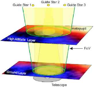
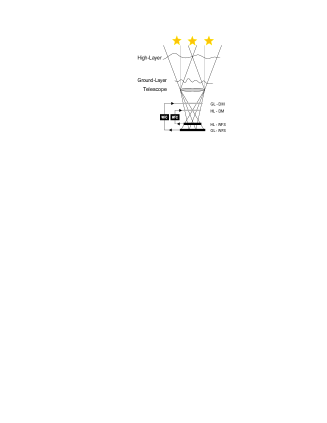
Figure 7.1: Left: Principle of Multi Conjugated Adaptive Optics correction. Several guide stars are used to probe the 3-dimensional structure of the atmosphere By illuminating the volume within the FoV and distinctive layers are corrected. A full correction for the higher layer is only guaranteed if this layer is fully covered by the footprints of the guide star metapupils. (Image taken from Kellner (2005)). Right: Schematics of the layer oriented MCAO approach with two layers. WFS, DM, and WFC are labels for the wavefront sensor, deformable mirror and wavefront computer for the high layer (HL) and ground layer (GL), respectively.

7.1.1 Star Oriented Approach

In the star oriented mode, each reference star is observed by one wavefront sensor and typically one detector. The information from the different directions of the guide stars is combined to generate 3D information of the atmosphere within the mapped FoV. In this approach of turbulence tomography (Tallon and Foy, 1990) the influence of a single layer can be computed and corrected with one deformable mirror conjugated to this layer. The first verification of this approach was done in an open loop measurement at the Telescopio Nazionale di Galileo (TNG) (Ragazzoni et al., 2000b).

7.1.2 Layer Oriented Approach

In the layer oriented approach (Ragazzoni et al., 2000a), each WFS and detector is conjugated to one layer in the atmosphere instead to a single star. The light of several guide stars is optically co-added to increase the SNR on the detector, such that also fainter stars can be used as guide stars. This increases the sky coverage, the fraction of regions on the sky that can offer a suitable asterism, substantially for this approach. Also the number of needed wavefront sensors and detectors is reduced, reducing the detector read-out-noise and the needed computing power compared to the SO approach. Only as many detectors are needed as layers are being corrected and not as many guide stars are used. Information from one WFS, and therefore one layer, can directly be fed to the corresponding DM. This results in a combination of independent control loops for the different layers and allows to adjust the integration time and bin size on the detector independently to the characteristics of the conjugated layer.
Distortions introduced by turbulence in layers close to the layer for which correction is attempted contribute stronger to the measurements than those from layers further away. The further away a layer, the more its introduced aberrations are smoothed out (Diolaiti et al., 2001).

A limitation of this approach can be the different brightnesses of the used guide stars. This can lead to an overestimation of the turbulence from a certain direction, when the light is co-added (Nicolle et al., 2004). An asterism of stars with similar brightness is therefore preferable.

7.1.3 Ground Layer Adaptive Optics

As already pointed out in Chap. 2.1 most of the turbulence in the atmosphere is generated in the ground layer. Correcting only this layer, one can remove the major contributor to the phase aberrations of the incoming wavefronts (Rigaut, 2002). Additionally, the correction is valid over a large FoV, as the light coming from different directions passes through the same region of turbulence near the ground, because of its small distance from the telescope pupil. In principle Ground Layer Adaptive Optics (GLAO) corrections can be operated by any MCAO system, operating just one single correction loop conjugated to the ground layer. In this context a Rayleigh Laser Guide Star (LGS), which is focused to about 5 - 10 km altitude, can be used, as it automatically illuminates only the ground layer and is not usable for correction of higher layers but still valid for ground layer corrections (Morris et al., 2004).

7.1.4 Current and Future MCAO Systems

Several MCAO instruments are planned and being built for different telescopes. The first on-sky tested MCAO system is the MAD instrument at the ESO/VLT. It will be described in detail in the next section.
At the Gemini South observatory on Cerro Pachon, Chile, a laser guide star assisted MCAO System, GeMS, is being installed with first light expected soon. The system will consist of 5 laser guide stars and additionally up to three natural guide stars. The single 50 W laser is split into five beams which are launched from behind the secondary mirror. The laser beacons will be located in the middle and the four corners of the $1.2\hbox{${}^{\prime\prime}$}\times 1.2\hbox{${}^{\prime\prime}$}$ FoV. Three deformable mirrors are going to be used to correct for turbulence in three layers: at ground level, 4.5 km and 9 km altitude. Shack-Hartmann wavefront sensors will be used in this star oriented MCAO approach.
The Fizeau-Interferometer LINC-NIRVANA for the Large Binocular Telescope (LBT) on Mt. Graham in Arizona, will be equipped with four layer oriented correction units, two for each telescope, which will correct the ground layer and a high layer (e.g. Farinato et al., 2008). In the so-called LINC mode the instrument will work with a classical single guide star AO system. In the later implementation phase called NIRVANA, the MCAO system will be able to use up to 12 NGS per side for the GLAO plus up to 8 NGS for the high layer adaptive optics correction (HLAO). The stars for GL correction can be located anywhere in a ring with an inner diameter of $2\hbox{${}^{\prime}$}$ and an outer diameter of $6\hbox{${}^{\prime}$}$ around the central science field of $10.5\hbox{${}^{\prime\prime}$}\times 10.5\hbox{${}^{\prime\prime}$}$ and the guide stars for the HLAO inside a circle with a diameter of 2 arcminutes.

7.2 MAD - Multi conjugated Adaptive optics Demonstrator

Figure 7.2: Examples for jitter offsets with MAD to scan the $2\hbox{${}^{\prime}$}\times 2\hbox{${}^{\prime}$}$ FoV. Left: Mosaic of 5 pointings covering the full $2\hbox{${}^{\prime}$}\times 2\hbox{${}^{\prime}$}$ FoV. Right: Jitter offsets for 5 pointings around the center of the FoV.

The ESO Multi conjugated Adaptive optics Demonstrator (MAD) is a prototype MCAO instrument, which was used to test different MCAO reconstruction techniques in the laboratory and on sky (Hubin et al., 2002; Marchetti et al., 2003; Arcidiacono et al., 2006). After extensive testing in the laboratory it was installed at the Nasmyth-focus platform of the ESO VLT UT3 telescope Melipal in the beginning of 2007. Because the instrument bench is fixed to the Nasmyth-platform, the pupil co-rotates with the field and an optical de-rotator at the entrance of the adaptive optics system is needed, as well as for the science camera.

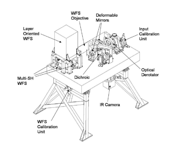
Figure 7.3: 3-dimensional view of the MAD bench with the major instrument components marked. The light beam enters at the de-rotator, passing the two deformable mirrors (DM) and is split by the dichroic into the IR part which is led to the science camera and the visible part which is led to the wavefront sensor objective. The layer oriented wavefront sensor is located above the star oriented multi Shack-Hartmann (SH) sensor.

MAD is designed to characterize the performance of both MCAO approaches, the star oriented one and the layer oriented one. It is optimized for corrections in the $\rm K^{\prime}$ band ($2.2\mu m$) over a circular $2\hbox{${}^{\prime}$}\times 2\hbox{${}^{\prime}$}$ FoV using natural guide stars (NGS). For the SO approach a multi Shack-Hartmann wavefront sensor, consisting of three movable Shack-Hartmann WFS (SHS) to look at any star present in the FoV, is implemented. SHS consist of a lenslet array that samples the incoming WF. Each lens forms an image of the guide star and the displacement of this image from a reference position gives an estimate of the slope of the local wavefront at that lenslet. The guide stars used for sensing the distortions should not be fainter than $m_{v}=14$. The layer oriented approach uses a multi Pyramid wavefront sensor (PWS) which is capable to sense up to 8 NGS simultaneously. The PWS consists of a four-sided glass pyramid which tip is located in the focal point of the telescope and it measures, similar to the SHS, the local slope of the wavefront. A uniform distribution of these stars is preferable but they can be everywhere in the $2\hbox{${}^{\prime}$}\times 2\hbox{${}^{\prime}$}$ FoV. The two different WFSs cannot be used simultaneously, a selector folds the light either to the SO-WFS or the LO-WFS.
Two deformable mirrors conjugated to the ground layer and a layer at 8.5 km altitude correct for the turbulence induced phase errors. A dichroic splits the light into an IR part ($1.0-2.5\leavevmode\nobreak\ \mu m$), led towards the science detector and a visual part ($0.45-0.95\leavevmode\nobreak\ \mu m$) led towards the wavefront sensor path. The CAMCAO (CAmera for MCAO) IR camera, built by the Faculdade de Ciências da Universidade de Lisboa (FCUL), is the science camera of MAD (Amorim et al., 2004). It consists of a $2k\times 2k$ Hawaii2 IR detector with a pixel scale of 0.028 arcsec/pixel and a FoV of $57\hbox{${}^{\prime\prime}$}\times 57\hbox{${}^{\prime\prime}$}$. The CAMCAO optics provide diffraction limited images down to the J ($1.25\leavevmode\nobreak\ \mu m$) band, and it is equipped with standard IR band filters for J ($1.25\leavevmode\nobreak\ \mu m$), H ($1.65\leavevmode\nobreak\ \mu m$), $\rm K_{s}$ ($2.2\leavevmode\nobreak\ \mu m$), Br-gamma ($2.165\leavevmode\nobreak\ \mu m$) and Br-gamma continuum. In Fig. 7.3 a detailed sketch of the layout of the instrument is shown. Unlike other instruments, with MAD the camera and not the telescope is moved to jitter within the field of view. Jitter movements are small offsets from the central pointing to avoid bad pixel coincidences on always the same position in the science field, to better estimate the sky background and/or to scan a larger FoV. The detector can cover the full $2\hbox{${}^{\prime}$}\times 2\hbox{${}^{\prime}$}$ FoV by moving into the four adjacent $1\hbox{${}^{\prime}$}\times 1\hbox{${}^{\prime}$}$ quadrants using linear x-y stages, see Fig. 7.2 for examples of jitter offsets for observations with MAD.

On sky testing of the star oriented mode was started in February/March 2007 with the first closing of the MCAO loop on March 25th (Marchetti et al., 2007). This first demonstration run consisted of 8.5 effective nights spread over 12 nights in total, with another demonstration run following for the SO mode. During the third demonstration run in September 2007 the LO mode was tested (Arcidiacono et al., 2008; Ragazzoni et al., 2008; Falomo et al., 2009). After the very successful demonstrations of the performance of MAD, three public science demonstration runs for the star oriented mode followed in November 2007, January 2008 and August 2008, where high resolution galactic as well as extragalactic science was performed (see e.g. Bouy et al., 2009; Wong et al., 2009).

7.3 Goal of this Work

The reason for analyzing MAD data was the uniqueness of this very first MCAO data. I want to analyze the stability of the multi conjugated adaptive optics correction regarding the potential achievable astrometric precision. MCAO observations offer the advantage of a big field of view with a resolution close to the diffraction limit. Although most of this advantage is seen in the enhancement in photometric studies, there are also some very interesting applications in the field of astrometry. Cluster dynamics, measuring velocity dispersions and common proper motions is just one of the many possibilities. Another very interesting case is the possibility of detecting the astrometric signal of a planetary companion orbiting its star. Limitations of today’s AO based searches are often the small FoV of classical AO imagers. Having an $1\hbox{${}^{\prime}$}\times 1\hbox{${}^{\prime}$}$ FoV with several reference stars will enable more precise astrometric measurements. But before starting with such science, one should check and analyze the performance of these systems, to see which effects this special kind of AO system has on astrometric measurements. When the first observations with such a system, the MAD instrument, were performed I had the chance to analyze some of these data. I decided to work with the data obtained in the layer oriented mode, as this will be the approach the future LBT instrument LINC NIRVANA will work with.
The goal of this work is to see how stable the AO performance of MAD is over time in terms of astrometric stability and to measure the achievable positional precision in the first MCAO layer oriented data.

Chapter 8 Astrometry with MAD

8.1 Observations

The observations analyzed here were conducted with the MAD instrument and the multi pyramid sensor in the LO mode. I analyzed data from two globular clusters, 47 Tucanae (NGC 104) and NGC 6388, which were observed during the demonstration run in September 2007 by our colleagues from the INAF Osservatorio Astronomico di Padova, Italy (Arcidiacono et al., 2008; Ragazzoni et al., 2008; Falomo et al., 2009). Due to bad luck with the observing conditions, these two sets are the best data obtained during the only layer oriented run carried out with MAD. In the case of the data of 47 Tuc I analyzed the data of the central $57\hbox{${}^{\prime\prime}$}\times 57\hbox{${}^{\prime\prime}$}$ FoV in the context of this work. In the case of the NGC 6388 cluster I analyzed a data set observed under good initial seeing conditions $0.46\hbox{${}^{\prime\prime}$}$), which lies at an outer part of the cluster. Another field in the center of the cluster was also observed, but with an initial seeing of $1.76\hbox{${}^{\prime\prime}$}$, which I did not analyze in this work. Unfortunately there will be no more data to compare my results with, as MAD is no longer offered.

I want to emphasize that the MAD instrument, as its name already says, was built to demonstrate that MCAO correction over a big field of view is possible. It did this with great success! But one also has to keep in mind, when interpreting the results shown in the next chapters, that this data is test data with all the possible problems during first observations. Not the full performance of this new AO correction technique can be expected, for this one has to wait for the next generation of MCAO instruments, which will be fully optimized. Nevertheless, this is the first attempt to analyze and characterize a layer oriented MCAO system with respect to its astrometric performance.

8.1.1 GLAO - 47 Tuc

The observations of the globular cluster 47 Tuc were obtained on September 22nd 2007 using only the Ground Layer Adaptive Optics (GLAO) approach. The center of the cluster, RA(J2000)=00:24:05.6, DEC(J2000)=-72:04:49.4, was observed in the Br-$\gamma$ filter. The camera was not moved during the exposures to scan the full FoV but instead stayed at the same position, observing a $57\hbox{${}^{\prime\prime}$}\times 57\hbox{${}^{\prime\prime}$}$ field. Four guide stars with magnitudes V = 11.9, 11.9, 12.4 and 12.5 mag, corresponding to an integrated magnitude of 10.63 (Arcidiacono et al., 2008), positioned around this field with one guide star in the lower left corner of this field were used to sense the wavefront distortions due to the atmosphere, see Fig. 8.1. Altogether I have 19 frames with NDIT = 15 exposures of an integration time of DIT $=2$ seconds. Each frame is averaged to correspond to a 2 seconds exposure. Seven sky frames were obtained before the cluster observation with the same values for DIT and NDIT and also averaged to frames with an exposure time of 2 seconds each. In Table 8.1 the observation is summarized together with the atmospheric conditions during the observations, indicated by the seeing value and the performance of the system indicated by the value of the fitted FWHM.

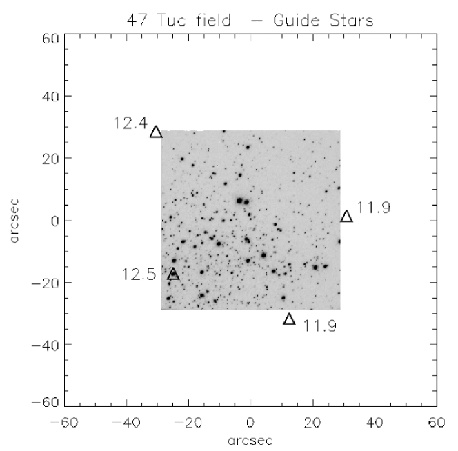
Figure 8.1: MAD image of the core of the globular cluster 47 Tuc. The triangles mark the positions of the AO guide stars relative to center of the observed FoV. The numbers close to the stars correspond to their F606W (visual) magnitude.

Object	frame	DIT	NDIT	rel. jitter		AO correct.	seeing [′′]	FWHM [′′]
				x	y		in $V$	in $Br_{\gamma}$
	1	2	15	0	0	GLAO	1.09	0.178
	2	2	15	0	0	GLAO	1.15	0.186
	3	2	15	0	0	GLAO	1.13	0.206
	4	2	15	0	0	GLAO	1.08	0.169
	5	2	15	0	0	GLAO	1.09	0.178
	6	2	15	0	0	GLAO	1.08	0.147
	7	2	15	0	0	GLAO	1.15	0.157
	8	2	15	0	0	GLAO	1.17	0.193
	9	2	15	0	0	GLAO	1.17	0.173
47 Tuc	10	2	15	0	0	GLAO	1.15	0.178
	11	2	15	0	0	GLAO	1.14	0.145
	12	2	15	0	0	GLAO	1.15	0.148
	13	2	15	0	0	GLAO	1.11	0.144
	14	2	15	0	0	GLAO	1.15	0.166
	15	2	15	0	0	GLAO	1.14	0.183
	16	2	15	0	0	GLAO	1.15	0.183
	17	2	15	0	0	GLAO	1.19	0.187
	18	2	15	0	0	GLAO	1.13	0.200
	19	2	15	0	0	GLAO	1.11	0.174

Table 8.1: Summary of the observations of the cluster 47 Tuc. The seeing value is measured by the DIMM seeing monitor in V band and the FWHM value corresponds to the one measured in the data (see Chap. 8.5)

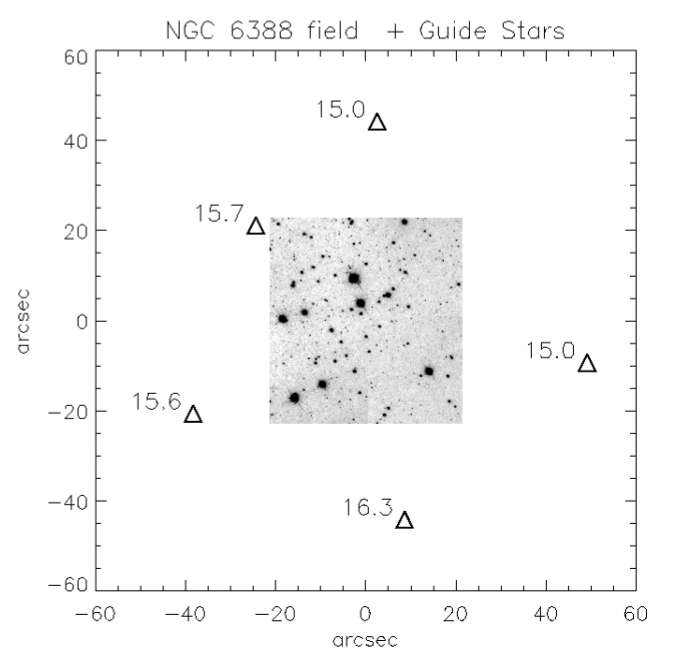
Figure 8.2: MAD image of the globular cluster NGC 6388. The triangles mark the positions of the AO guide stars relative to center of the observed FoV. The numbers close to the stars correspond to their F606W (visual) magnitude.

8.1.2 MCAO - NGC 6388

The data of the globular cluster NGC 6388 was obtained on September 27th 2007 using the full MCAO capability of MAD. The observations are in the $K_{s}$ filter using 5 guide stars with $V=15.0,15.0,15.6,15.7$ and 16.3 mag, corresponding to an integrated magnitude of 13.67 (Arcidiacono et al., 2008). The field together with the guide stars is shown in Fig. 8.2. The observed field lies at the lower left corner of the cluster at RA(J2000)=17:36:22.86, DEC(J2000)=-44:45:35.53. All together 30 frames were obtained, the first five in GLAO and the last 25 in full MCAO. A jitter pattern of five positions was used, repeated six times with three slightly different central points, to scan part of the $2\hbox{${}^{\prime}$}\times 2\hbox{${}^{\prime}$}$ FoV (Fig. 8.3). The first 10 frames were obtained with DIT = 10 seconds and NDIT = 24, and in the last 20 frames the number of exposures was reduced to NDIT = 12. All frames are averaged to correspond to a 10 second exposure.

Object	frame	DIT	NDIT	rel. jitter		AO correct.	seeing [′′]	FWHM [′′]
				x	y		in $V$	in $K_{s}$
	1	10	24	0	7	GLAO	0.43	0.098
	2	10	24	5	12	GLAO	0.41	0.094
	3	10	24	5	2	GLAO	0.49	0.099
	4	10	24	-5	12	GLAO	0.55	0.094
	5	10	24	-5	2	GLAO	0.51	0.090
	6	10	24	0	7	MCAO	0.41	0.095
	7	10	24	5	12	MCAO	0.38	0.097
	8	10	24	5	2	MCAO	0.37	0.098
	9	10	24	-5	12	MCAO	0.39	0.103
	10	10	24	-5	2	MCAO	0.40	0.106
	11	10	12	2	5	MCAO	0.45	0.126
	12	10	12	2	5	MCAO	0.43	0.117
	13	10	12	7	10	MCAO	0.45	0.130
	14	10	12	7	10	MCAO	0.50	0.158
NGC 6388	15	10	12	7	0	MCAO	0.51	0.130
	16	10	12	7	0	MCAO	0.49	0.155
	17	10	12	-3	10	MCAO	0.48	0.170
	18	10	12	-3	10	MCAO	0.49	0.140
	19	10	12	-3	0	MCAO	0.45	0.119
	20	10	12	-3	0	MCAO	0.41	0.133
	21	10	12	-3	6	MCAO	0.42	0.120
	22	10	12	-3	6	MCAO	0.44	0.131
	23	10	12	2	11	MCAO	0.54	0.139
	24	10	12	2	11	MCAO	0.56	0.158
	25	10	12	2	1	MCAO	0.43	0.176
	26	10	12	2	1	MCAO	0.50	0.153
	27	10	12	-8	11	MCAO	0.46	0.143
	28	10	12	-8	11	MCAO	0.48	0.135
	29	10	12	-8	1	MCAO	0.47	0.120
	30	10	12	-8	1	MCAO	0.47	0.134

Table 8.2: Summary of the observations of the cluster NGC 6388. The seeing value is measured by the DIMM seeing monitor in V band and the FWHM value corresponds to the one measured in the data (see Chap. 8.5)

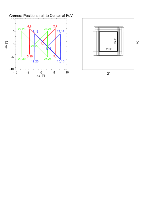
Figure 8.3: Left: Jitter pattern of the observations of NGC 6388. The offsets are in seconds of arc and relative to the center of the FoV. The numbers indicate the frame which was taken at that position. Note the change of taking two images at one position for frames 11-30 and then moving to the next jitter position instead of taking one frame per position and execute the jitter pattern twice for frames 1-10. Right: Frames taken in the $2\hbox{${}^{\prime}$}\times 2\hbox{${}^{\prime}$}$ FoV and the finally cut-out area common to all frames drawn with thick lines. This common area was used to investigate the astrometric precision.

After the science frames, five sky frames were taken outside the cluster using the same jitter pattern as in the science frame. At each position 24 frames with 10 seconds exposure time, averaged to one frame of 10 seconds each, were obtained.

In Table 8.2 the observations are summarized together with the atmospheric conditions during the observations, indicated by the seeing value.

8.2 Data Reduction

NGC 6388

Each science frame of the NGC 6388 cluster data was flatfielded by the flatfield image obtained from sky flats at the beginning of the night and badpixel corrected, by replacing the marked pixels with the median of the pixels themselves and their 8 nearest neighbors, with a badpixel mask obtained from the same flat-field images. I did not create the flatfield and badpixel mask by my own in this case, but used those made by our colleagues from Italy. A description of how these frames were created can be found in (Moretti et al., 2009). Briefly, the obtained sky flats were median combined to one flatfield and also used to create the badpixel mask.

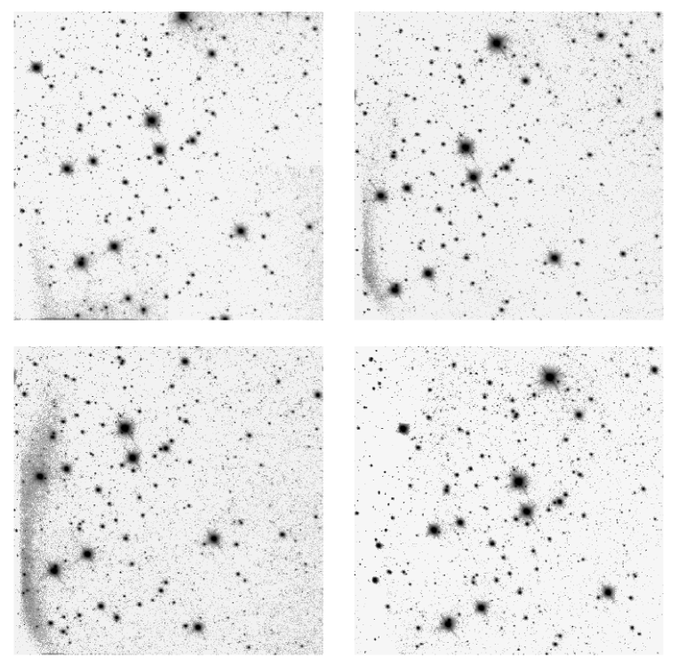
Figure 8.4: Arc in the MAD frames produced by unshielded and unfiltered reflected light. Several examples from different jitter positions show the intensity dependence of this arc on the jitter position. Some frames have a prominent arc, whereas it is not visible in others.

Sky subtraction was done by median combining all sky and science frames to get one single sky frame. Using only the sky frames obtained right after the science frames to create the sky frame, did not work satisfactorily. As only five sky-frames were available, the remaining stars in the frames did not average out perfectly, leaving small holes in the science frames after subtracting the sky frame. Also $\kappa-\sigma$ clipping did not yield a satisfactory result. Using all science frames together with the sky frames to create a median image for the sky estimation yielded the best result. Therefore, this resulting image was used for sky subtraction. This sky frame was then normalized to the median counts of the science frame before subtraction.
Additionally, NaN and infinite values which were still in the frames after the data reduction, were substituted by the median of their 8 nearest neighbors, as the routines for the following analysis had problems with such pixel values.
In the first demonstration runs with MAD a problem occurred. Unfiltered light was reflected on the instrument bench and could enter the science camera, producing a banana like arc on the lower left side of the images. The intensity and position of this arc depends on the position of the camera while jittering to scan the FoV. This reflection could be avoided in the later science demonstration runs by shielding the camera entrance with a tube. Nevertheless, I see this arc in the images, see Fig. 8.4. As it is position dependent, the arc cannot be removed with the flatfield correction or sky subtraction. The distribution of the arc is always close to the border of the detector and only affecting a small portion of the stars. While this extra, unshielded light is for sure a problem for photometry, its influence on the astrometric positions of the stars may be small. Nevertheless, I tried to avoid stars, affected by the arc in my analysis.

In the case of the NGC 6388 data, jittering was used during the observations and I cut the images to the common FoV which was part of all images after the data reduction. That left us with a slightly smaller field of the size of $1517\leavevmode\nobreak\ \rm\leavevmode\nobreak\ px\times 1623\leavevmode\nobreak\ \rm\leavevmode\nobreak\ px$ ($42.5\hbox{${}^{\prime\prime}$}\times 45.4\hbox{${}^{\prime\prime}$}$), see Fig. 8.3, right panel. Only the stars in this common field are taken into account for the following astrometric analysis.

47 Tuc

In the case of 47 Tuc no flat-field images were taken in Br$\gamma$ (central wavelength $=2.116\mu m$) in that night. As I had no other choice I used the same flatfield image for correction as for the NGC 6388 data observed in $K_{s}$ (central wavelength $=2.15\mu m$), assuming that the pixel to pixel variations are the same or very similar in these two filters, whose central wavelength is not too different. As the data I got from our collaborators for the cluster 47 Tuc was already sky subtracted and corrected for the reflecting arc, I only corrected for the flatfield, badpixel and NaN and infinite pixel values in the same way as for the NGC 6388 data. The data of 47 Tuc was obtained without moving the camera. All frames contain the same field and I did not cut the single frames.

8.3 Strehl Maps

As a check of the AO performance I calculated Strehl-maps for each frame. A theoretical diffraction limited PSF for MAD was computed and normalized to a flux of one. With the Source Extractor package (Bertin and Arnouts, 1996) the stars in the frame were detected and aperture photometry was used to calculate the flux of the stars. After normalizing the flux to one, a comparison of the theoretical peak value and the maximum value of the star yields the Strehl ratio. After interpolating values for areas where no stars were found a smooth surface was fitted to the data, leading to a two dimensional Strehl-map for each frame. In Fig 8.5 and 8.6 some of these Strehl-maps are shown, the first, middle and last frame.

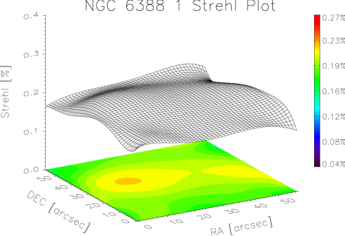
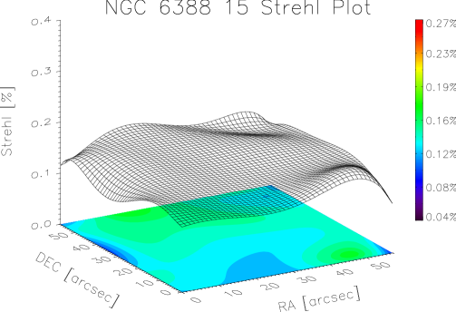
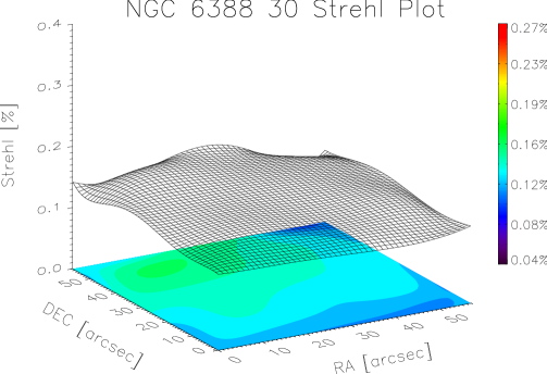
Figure 8.5: Strehl-maps for some of the mad frames of the cluster NGC 6388. Shown are the first (GLAO), middle and last exposure (both MCAO). The degradation in performance with time, as described in the text, can be seen.

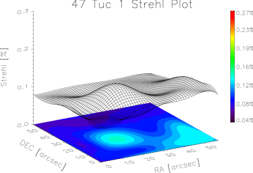
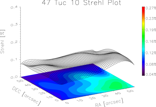
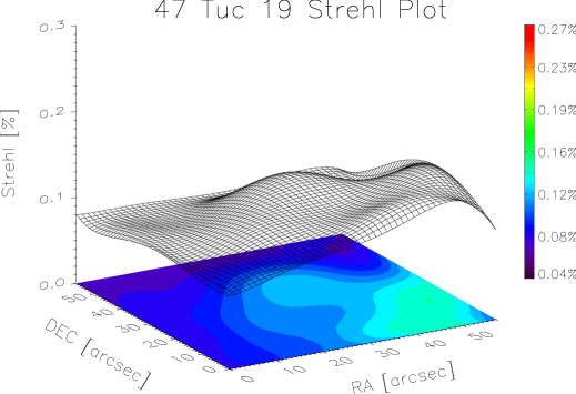
Figure 8.6: Strehl-maps for some of the mad frames of the cluster 47 Tuc obtained with GLAO. Shown are the first, middle and last exposure.

In the case of NGC 6388 a slight degradation in performance with time can be seen, following roughly the change in the seeing. The first five frames obtained with GLAO have the highest Strehl ratio and do not change with the changing seeing conditions. The Strehl is fairly even over the field of view of the camera with a small drop-off to the edges of the field. This shows how well and uniformly the layer oriented MCAO approach corrects wavefront distortions. The drop-off to the edges of the FoV can partly be explained by the MCAO and the atmospheric tomography approach. The light coming from the different directions of the guide stars is optically co-added and a correction is computed based on this light distribution. But the footprints of the columns above the telescope in the direction of the guide stars overlap more in the middle of the field than at the edges in the higher layer. If the control software is not optimized to correct over the whole FoV very evenly, the middle of the field will be corrected better. As the data I am looking at is the first data of MCAO and layer oriented mode, I am not surprised to see such an effect. A performance evaluation of these data can be found in Arcidiacono et al. (2008). In the case of 47 Tuc the Strehl is smaller than in the case of the NGC 6388 data. The main reason for that is not that this data is taken with correcting only the ground layer, but more due to the circumstance that already the initial conditions for the AO correction was very poor with a seeing of 1.09 - 1.19 arcseconds. An AO system can only enhance the performance significantly, if the initial atmospheric conditions are fairly good. Nevertheless, an even Strehl ratio of $\sim 15\leavevmode\nobreak\ \%$ over a $1\hbox{${}^{\prime}$}\times 1\hbox{${}^{\prime}$}$ FoV is already an enhancement compared to the seeing limited case.

8.4 PSF Tests

Before I decided what kind of model or empiric PSF I should use to fit the positions of the stars in the frames, I conducted several tests of the PSFs in the frames. I analyzed the distributions of shape and orientation of the PSF over the field of view, to check if I can fit the same PSF to all stars or have to use different PSFs for different parts of the FoV, which is mostly the case in classic single guide star adaptive optics imaging. As I first only had the data of the cluster NGC 6388, I conducted all these PSF tests with this data set and based the following decisions and steps on the consequential results. Later, after the analysis of the NGC 6388 data set was finished, I got the opportunity to also analyze GLAO data of the cluster 47 Tuc for which I conducted the same tests. Though they show certain differences, I nevertheless analyzed this data set in the same way as the NGC 6388 data, to conserve the possibility of a direct comparison of the results of the two data sets.

Figure 8.7: Distribution of the orientation and eccentricity of the PSF in one of the MCAO frames of the NGC 6388 data as an example. The upper panels show the distribution as function of the distance of the stars from the center of the detector. The middle panels the distribution as function of the distance in x-direction and the lower panels as function of the y-distance.

For the PSF tests I first used the StarFinder program (see next section for details) to measure the positions of the stars in the field. I then cut a quadratic box around each star and fitted a two dimensional, rotatable Moffat function (see Equ. 4.1) to each star, using the non-linear least square fitting package MPFIT2DPEAK, provided by Craig Markwardt (Markwardt, 2009). After flagging those stars which were too close to the frame edges or other stars, as well as those where the fit with the Moffat function obviously gave wrong parameters, I worked with the remaining 780 - 800 stars in both data sets. The fitting routine has some problems if more than one star is present in the box cut around the star which one wants to fit. If the two stars have similar brightness, the valley between them is fitted and if the second star is brighter than the one gained for, always the brighter one is fitted. I therefore checked for large changes in the position and brightness of the fitted Moffat function to the values given by StarFinder and flagged those stars where the fit did not went well.

Looking at the distribution of the rotation angle $\Theta$ of the fitted Moffat function, a small dependency of the orientation of the PSFs with the position of the stars can be seen in the case of the NGC 6388 data. The angle is measured clockwise from the detector x-axis to the major axis and is in the range $[-\frac{\pi}{2},\frac{\pi}{2}]$. In Fig. 8.7, left panels, an example of the distribution of the orientation of the PSF is shown for one frame of the MCAO frames of the NGC 6388 data. The upper panel shows the distribution as function of the distance of the stars from the center of the detector. The middle panel the distribution as function of the distance in $x$-direction and the lower panel as function of the $y$-distance. Although it seems, that fewer orientations near $\Theta=0\hbox{${}^{\circ}$}$ are fitted, this effect is not dependent on the distance of the stars from the center. I calculated correlation coefficients for these plot, yielding values of 0.019, 0.438 and -0.093 for the distance from the center, the $x$-direction and the $y$-direction respectively. Whereas the coefficients for the center distance and the $y$-direction are not significant, the one for the $x$ direction shows a moderate correlation. I plotted the fitted Moffat functions as enlarged ellipses overimposed on the positions of the stars. Fig. 8.9 shows the distribution in the right panel. One can see the different orientation of the stars in the lower right corner compared to the ones in the upper left corner. This behavior changes only slightly over the different frames. In the case of plotting angles, one has to be careful with the interpretation of the correlation coefficient, because of the periodicity of the angle. Plotting the distribution with different cut values, as for example $[0,\pi]$ or $[\frac{\pi}{2},\frac{3}{2}\pi]$, can yield different correlation coefficients. I therefor calculated the coefficient for different cut values. The correlation coefficients changes slightly, but yielded all to the same interpretation as above.

Figure 8.8: Correlation of the eccentricity and orientation of the PSF in one of the MCAO frames of the NGC 6388 data.

I also looked at the shape, i.e. the eccentricity, of the fitted Moffat functions. In Fig. 8.7, right panels, the distribution of the eccentricity, $e=\frac{\sqrt{a^{2}-b^{2}}}{a}$ as a function of distance to the detector center is shown. Here $a$ is the half width at half maximum (HWHM) of the larger axis and $b$ the HWHM of the smaller axis. Although the mean eccentricity is $\sim 0.4$, no dependency of the shape of the PSF with the position of the stars on the detector is observable. The calculated correlation coefficients are 0.125, -0.216 and 0.115 for the distance from the center, the $x$ direction and the $y$ direction respectively. All these values show a very weak correlation. I also looked at the distribution of the eccentricity in the four quadrants of the detector, to check if there is any correlation, as for example one of the guide stars is located close to the upper left quadrant for the NGC 6388 observations (see Fig. 8.2). Each quadrant shows a similar distribution of eccentricities.

As a last check I looked for a correlation between the orientation of the PSF and its eccentricity. As one can see in Fig. 8.8 there is no preferred eccentricity for a specific angle.

Compared to the single guide star AO correction, where the stars are elongated in the direction to the guide star and the effect is stronger the further away the star is from the guide star, these results already show the advantage and improvement of observing with MCAO.

Figure 8.9: Fitted Moffat functions, displayed as enlarged ellipses at the positions of the stars, showing the orientation and shape of the PSFs in the 47 Tuc data in the left panel. The different sizes of the ellipses reflect the different fitted FWHM of the Moffat functions. The red ellipse marks the guide star contained in the detector FoV. For comparison the same plot is shown for a MCAO frame of the NGC 6388 data in the right panel with the same enlargement factor.

And although I see some small spatial correlations, I decided to use one PSF model to fit all stars in the field in the way as described in the next section (8.5). Using the Moffat fit in all frames was also not an option, because of the above mentioned fitting problems with close stars pairs.

Figure 8.10: Distribution of the orientation and eccentricity of the PSF in one frame of the 47 Tuc data as an example. The upper panel shows the distribution as function of the distance of the star from the center of the detector. The middle panel the distribution as function of the distance in x-direction and the lower panel as function of the y-distance.

When I later analyzed the data of the cluster 47 Tuc, I performed the same tests. As the initial observing conditions were worse than in the case of the NGC 6388 data, also the overall performance was a bit worse (compare Tables 8.1 and 8.2 and Figs. 8.5 and 8.6). Already in the image one can see an elongation of the stars in one direction. The analysis of the orientation of the fitted Moffat function confirms this impression, see Fig. 8.10. A clear preference of orientation angles between $\Theta=-30\hbox{${}^{\circ}$}$ and $\Theta=-50\hbox{${}^{\circ}$}$, with an average of $\overline{\Theta}=-43.5\hbox{${}^{\circ}$}$, is recognizable, with a small dependency on the $y$-positions of the stars in the field. Stars in the upper part of the detector seem to be oriented a bit more to the y-direction than the stars in the lower part of the field, see also Fig. 8.9. The eccentricity distribution, with a mean eccentricity of 0.55, also does only show a very weak dependency on the position on the detector. But the mean eccentricity is higher than in the case of the NGC 6388 data obtained under good initial conditions. One of the used guide stars is in the lower left corner of the FoV. If the shape of the stellar PSFs depended on the position of this guide star, $\Theta$ should change over the field depending on the position angle between the stars and the guide star. Instead the guide star itself is elongated and oriented in the same way as the stars around it ($\Theta=30.25\hbox{${}^{\circ}$},e=0.59$). In the left panel of Fig. 8.9 the fitted Moffat functions are displayed as ellipses at the positions of the stars, showing the orientation and shape of the PSFs. This shows nicely the principle of the layer oriented correction approach, where the light of all guide stars is added and measured for the correction of a certain layer and the correction itself is not so much dependent on the single position of the guide stars, as in the classical, single guide star approach. On the other hand it also shows, that the correction was not yet perfect in this data set, leaving this residual elongation and orientation of the stars.

Nevertheless I continued measuring the positions of the stars and their uncertainties in the same way as in the case for the data of the cluster NGC 6388 to compare the two sets later under the aspect of GLAO versus MCAO correction. Most of the stars in the 47 Tuc data show the same orientation and eccentricity, making it again feasible to work with one PSF model for the full FoV.

8.5 Position Measurements

To measure the positions of the stars in the single images of both clusters I used the program StarFinder (Diolaiti et al., 2000b, a), which is an IDL based code to analyze AO images of stellar fields. The following description is for 47 Tuc, but it is the same for the NGC 6388 data.

I directly extracted the Point Spread Functions (PSF) for the star fits from the images, by using in each frame the same 30 stars. In Fig. 8.11 the stars used for the PSF extraction are marked for both fields.

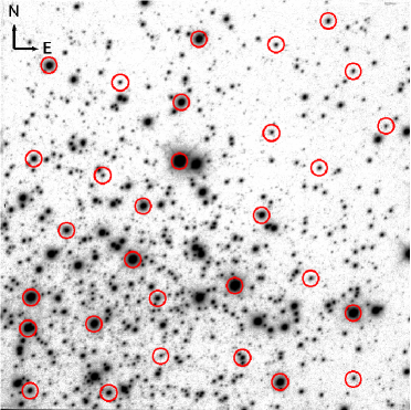
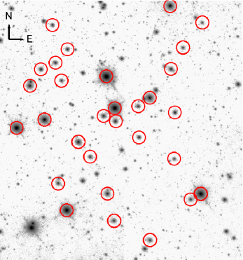
Figure 8.11: Stars used for PSF extraction in the fields 47 Tuc (left) and NGC 6388 (right). Note the different scales: The 47 Tuc field is $57\hbox{${}^{\prime\prime}$}\times 57\hbox{${}^{\prime\prime}$}$ and the NGC 6388 field is cut to $42.5\hbox{${}^{\prime\prime}$}\times 45.4\hbox{${}^{\prime\prime}$}$.

I assumed here that the PSF does not vary strongly over the FoV, as would be the case in single guide star adaptive optics. But as seen in the analysis before (Sect. 8.4), the PSF did not show a huge variation over the field and as I do not intend to do photometry, I assume that the center of the PSF can still be determined accurately enough from a fit with an averaged PSF. In Fig. 8.12, (left), an example of such an extracted PSF is shown. The flux is normalized to one. The 30 stars were chosen to be equally distributed over the entire field and to give a good mixture of brighter and fainter stars. After marking the stars, StarFinder provides the opportunity to remove secondary sources such as close stars, which may be in the box cut around the marked stars. The final PSF is then generated by a median combination of the selected stars. At the end I cut the square box containing the PSF into a round one of 80 pixel diameter, which corresponds more to the base of a PSF.
Some of the brighter stars are saturated. In the case of MAD with its IR detector these saturated stars do not have a flat plateau in place of the PSF tip, but instead have a hole in the middle (Fig. 8.12, right).

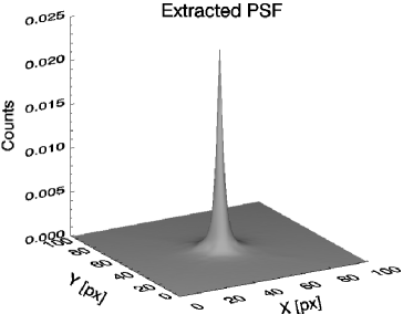
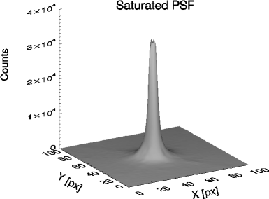
Figure 8.12: Left: Example of a with StarFinder extracted PSF. The flux is normalized to one. Right: Example of a saturated PSF. The PSF has a hole instead of a tip. The different peaks at the ’top-ring’ can clearly be seen, causing StarFinder to fit several stars instead of one.

StarFinder had some problems, fitting those stars, as the remaining ring of the PSF is not constant in flux. Several stars were fitted along the ring. In principle it should be possible to also fit the extracted PSF to the saturated stars by first filling the holes and then using a function of StarFinder, which repairs the PSF during the fit. But as it is difficult to evaluate how the position measurement is affected by this procedure and I had only a few saturated stars in the field, I decided to not use these stars in the following analysis. After deleting the false detections in all frames, $\sim 1450$ stars remained in the 47 Tuc data and $\sim 1500$ stars in the first 10 frames of the NGC 6388 data and $\sim 600$ in the last 20 frames. The huge difference in the numbers for the NGC 6388 data is due to the change in integration time after the first 10 frames (see Tab. 8.2), that led to a lower signal to noise ratio in the averaged frame and therefore to fewer detections of the faint stars.

The position uncertainties for the stars were computed with photon statistics as an estimate. The extracted PSF from each frame was cut at the value of half maximum. Then a rotatable ellipse was fitted to the slice-plane, giving values for the semi-major and -minor axes of this ellipse, corresponding to the HWHM of the two axes. After parametrization the ellipse equation I calculated the maximum projection values, $x_{max},y_{max}$, of the semi-major axis onto the $x$- and $y$-axes. The positional errors, $\Delta x,\leavevmode\nobreak\ \Delta y$, for the single stars of each frame were then computed following photon statistics by:

$$\Delta x =\frac{x_{max}}{\sqrt{n}}$$ (8.1)

$$\Delta y =\frac{y_{max}}{\sqrt{n}}$$

where $n$ is the total number of photons. To derive $n$ one has to take into account the gain factor of the detector, $g=2.9\rm e^{-}/ADU$ for the CAMCAO camera, and the number of exposures, NDIT, averaged to create this frame. In Tab. 8.1 and 8.2, last column, the mean FWHM value, calculated as the mean of the FWHM of the minor- and major-axis, is noted. This approach is somewhat conservative compared to the classical approach, calculating the error by $\sigma/\sqrt{n}$, but I did not want to underestimate the errors. The positional errors from the fit derived like this range from 0.010 mas (0.00034 px) to 0.555 mas (0.020 px) for the brightest and faintest star, respectively, in the 47 Tuc data set and from 0.004 mas to 0.141 mas (0.0001 - 0.005 px) in the NGC 6388 data set. The difference in these values for the two data sets comes mainly from the smaller FWHM of the PSFs in the NGC 6388 data, which itself is mainly due to the better initial observing conditions.

8.6 Ensquared Energy

In adaptive optics observations often the encircled or ensquared energy is taken as a measure of performance besides the FWHM. The encircled energy in percent is defined as the flux of a PSF contained in a certain radius from the middle point divided by the total flux. In the case of an image where the flux is given as flux per pixel, like any detector image, the ensquared energy is used, which is the flux within a certain quadratic box with the size of $n$ pixel times $n$ pixel. To correctly calculate the comprised flux one needs to know how the program used to calculate the ensquared energy, defines the pixel center. I used IDL in my analysis, where a pixel is defined from -0.5 to 0.5. For instance, a peak of a PSF given by the coordinates 50, 50 is therefore defined in the middle of the pixel and not for example at its lower left corner. Knowing this, I measured the flux in square boxes with $1\times 1,\leavevmode\nobreak\ 3\times 3,\leavevmode\nobreak\ 5\times 5...79\times 79$ pixel in diameter, covering the full size of the extracted PSFs. In Fig. 8.13 (left), an example of the development of the ensquared energy with pixel distance from the center pixel is shown. Here radius denotes the half diameter of the box. Finally I calculated the radius in pixels within which 50% of the energy of the PSF is contained and used this radius as a performance indicator. The smaller the radius the better the AO correction, moving flux from the seeing halo of the PSF into the central peak. As comparison I show in Fig. 8.13, right panel, the relation between the measured FWHM of the PSF and the radius of 50% ensquared energy, $r_{50}$. Clearly visible is a relation, the larger the FWHM, the larger $r_{50}$. For the MCAO data this relation is sharper and better defined as for the ground layer data, reflecting the better initial observing conditions and therefore the better correction in the single frames.

Figure 8.13: Left: Example of the development of the ensquared energy with box size for the MCAO and the GLAO case. The radius containing 50% of the energy is marked. Right: Relation between measured FWHM and radius containing 50% of the energy for the MCAO and GLAO correction.

8.7 Distortion Mapping

To investigate the stability of the MCAO and GLAO performance in terms of astrometric precision over time, I first had to correct for distortions of the field. During the observations problems with the de-rotator occurred due to a software problem, leading to a bigger rotational error in several frames. If the AO correction is very stable over time, the relative positions of the stars should be the same after correcting for effects such as the de-rotator problem.
The first thing I did, was to set up a coordinate reference frame to which I mapped the single frame coordinates. For this I set up some criteria for the stars chosen to create this reference frame: After the measurement of the positions of the stars in each field following the procedure described in Sect. 8.5, I compared the lists of stars found in the individual frames and identified the subset common to all frames of the NGC 6388 and 47 Tuc data, respectively. The next step was to exclude faint stars from the list, namely those that had less than 10000 counts, i.e. a peak value around 85 ADU in the case of 47 Tuc and those with less than 2800 counts, peak $\sim 50$ ADU, in the case of NGC 6388. These values were chosen, because in the NGC 6388 data there are fewer bright stars than in the 47 Tuc data. Additionally, all stars that have a close neighbor at less than 2 HWHM separation were excluded. This left $\sim$ 280 stars for the 47 Tuc field and $\sim$ 130 stars for the NGC 6388 field, still absolutely enough to calculate the transformations.
In order to create the reference frame, I started to use the best frame I had, chosen according to the highest mean Strehl in the images, as a first reference frame and mapped all the positions from each individual frame onto this reference frame. I then calculated the shift and scale in $x$ and $y$ and the rotation between these frames using the MIDAS

data reduction software and simple affine transformations. I was not applying any interpolation directly to the images, but instead just worked with the measured coordinates. After correcting for the derived rotation, as well as for the shift and scale in $x$ and $y$ of each stellar position I created a master-coordinate-frame by averaging the position of each star over all frames. This was my new masterframe for the coming analysis. I then mapped all coordinates from each frame to this masterframe, leading to a better transformation. One could think that one can get even better transformations between the frames by applying this method iteratively, creating once more a master-coordinate-frame by calculating mean positions and averaging those positions. If the distortions in the images, left over from the AO or systematic, were homogeneous over the FoV the transformations should not change or enhance a lot. But if the distortions are not homogeneous, but depend, for example, on the camera position in the FoV, I would introduce warpings in the master-coordinate-frame which I cannot map with a simple shift, scale and rotation anymore. I therefore stopped after one iteration.
I then calculated the residual separations between the positions of the stars in the master-coordinate-frame to the new positions in every frame calculated with the obtained transformation parameters and analyzed them as a measure of astrometric precision.

Chapter 9 Results

To set my results concerning the astrometric precision achievable with MCAO into a context, I looked at overall performance indicators, such as the FWHM of the fitted PSF and seeing. This led to several interesting results. In Fig. 9.1 I have plotted the FWHM calculated from the extracted PSF over the measured mean DIMM seeing for each frame. The seeing is measured in the $V$ band, while the observations were made in $Br_{\gamma}$ (47 Tuc) and $K_{s}$ (NGC 6388). Hence the difference between the seeing and the measured FWHM cannot be directly taken as the correction factor achieved. Nevertheless, the principal relation between these two values is preserved as Fig. 9.1 demonstrates. In the case of the NGC 6388 data (right panel), where the first 5 frames were obtained with GLAO correction and the last 25 with full MCAO correction, I marked the GLAO frames in red. Interestingly, the FWHM does not change significantly in the GLAO frames, although the seeing does, but in the MCAO case, I see a correlation between seeing and FWHM, as expected. A similar behavior of the FWHM can be seen in the 47 Tuc data, which is also in ground layer mode. The FWHM gets only slightly larger, the larger the seeing does. On the one hand the different FWHM values for nearly the same seeing may be explained by slightly different eccentricities of the PSFs in the different frames, leading to different mean FWHM values when calculated as the mean of the FWHM values of the minor- and major-axes. On the other hand, this can be interpreted as a sign of the non-correlation of these two parameters during GLAO correction. But this has to be seen with caution, as I have no other data set confirming or disproving this interpretation. A possible reason for the behavior in the NGC 6388 data is that the AO system was optimized for the ground layer correction in the nights before. The GLAO correction alone worked very well and even better than expected. Switching on the full MCAO correction can in a first attempt lead to a small degradation in the performance, if the controller of the system has not yet been optimized for the correction of two layers. Also in the case of MAD, the subsystems for the correction of the two layers are nested, meaning that one sensor 'sees 'the correction applied to the distortions of the other layer. This could lead to a degradation of the overall performance, if the system is not yet fully optimized. As this is the first time the full MCAO approach was tested, this resulting behavior of the performance is interesting but comprehensible and should not lead to wrong conclusions about the full capacity of the MCAO correction. To analyze this behavior further, one would need more data and more detailed information about the applied correction parameters of the system, both of which we do not have. Also our goal is not a performance analysis, this is done by the group that built the layer oriented part of MAD (Arcidiacono et al., 2008), but to see how precise astrometric measurements can be conducted under the given observing circumstances and corrections. Altogether the seeing does not change a lot during the observing time in both cases, but rather varies between $1.08\hbox{${}^{\prime\prime}$}-1.19\hbox{${}^{\prime\prime}$}$ in the case of the 47 Tuc data and $0.37\hbox{${}^{\prime\prime}$}-0.56\hbox{${}^{\prime\prime}$}$ during the NGC 6388 observations (see also Tables 8.1 and 8.2).

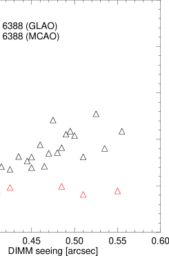
Figure 9.1: FWHM over seeing plotted for the 47 Tuc (left) and NGC 6388 (right) data. The five ground layer frames are marked in red in the right panel with the NGC 6388 data.

9.1 Separation Measurements

One test I performed, was to measure the relative separation between various pairs of stars all over the FoV. I wanted to derive a time sequence of the separation, to see how stable it is. If only a steady distortion were present in the single frames, then the separations should be stable over time or only scatter within a certain range given by the accuracy of the determination of the position of the stars. If differential distortions between the single frames are present, but these distortions are random, the scatter of the separations should increase. A not perfectly corrected defocus for example would change the absolute separation between two stars, but, to first order, not the relative one measured in the frames, if this defocus is stable. An uncorrected rotation between the frames would change the separation of two stars in the x and y direction, but not their full separation, $r$.

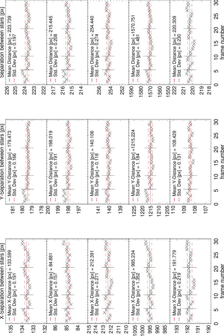
Figure 9.2: Separation between pairs of stars plotted against frame number. The left panel shows the separation in x-direction, the middle panel in y-direction and the right panel the full separation $r=\sqrt{\Delta x^{2}+\Delta y2}$. The small straight lines mark the frames after which a new five points sequence of jitter movements was started.

Performing this test for several stars with short and large separations and with different position angles between the stars showed in the case of the NGC 6388 data a recurring pattern in the separation in $x,y,r$, which is not observable in the 47 Tuc data. Fig. 9.2 shows the separation in $x,y$ and $r$ over the frame number for five representative pairs of stars in the NGC 6388 data. Looking at the pattern, which repeats after five frames for the first 10 frames and after 10 frames for the following frames (where always two images were taken at the same jitter position before moving to the next position), this change in separation seems to be correlated with the jitter movement during the observations which also has a five points pattern with an additional change of center position (see Fig. 8.3). In the case of the MAD instrument the camera itself is moved in the focal plane to execute the jitter pattern. This can lead to vignetting effects, if the jitter offset is too large and it seems to introduce distortions dependent on the position of the camera in the field of view. It is unlikely that this pattern is due to the problems with the de-rotator, because of the uniform repetition of the pattern. Also this pattern is not seen in the 47 Tuc data, which was obtained without jitter movements, but experienced the same de-rotator problems.
I performed this test with the same star pairs after applying the calculated distortion correction for shift, scale and rotation (see Sect. 8.7). The strong pattern is gone, leaving a more random variation of the separation. Also the calculated standard deviation is much smaller, ranging from a factor of $\sim 3$ up to a factor of $\sim 19$ times smaller! Comparing the single standard deviations shows a smaller scatter among their values than before the distortion correction. All this yields to the conclusion, that the calculated and applied distortions remove a large amount of the separation scatter, but not all of it. The remaining scatter of the separations between the stars in the single frames still ranges from $\sim 1.2-2.8$ mas, well above the scatter expected from photon statistics, pointing to uncorrected higher order distortions. But the values here are only calculated for a small fraction of the stars in the frames. I therefore also had a look on a more global scale of the positional residuals.

9.2 Residual Mapping

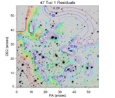
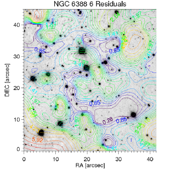
Figure 9.3: Example contour plots of the residuals (in mas) of the positions of the stars after the distortion correction in the upper panels. In the lower panels, the corresponding arrow maps are shown. The arrows are extended by a factor of 1000. The left panels show the data of the cluster 47 Tuc and the right panels the data of the cluster NGC 6388. The empty areas in the 47 Tuc data are due to the applied selection criterias for the stars.

To look at the spatial distribution of the residuals after the distortion correction, where I corrected for $x\rm and\leavevmode\nobreak\ y$-shift, $x\rm and\leavevmode\nobreak\ y$-scale and rotation relative to the masterframe, I created contour plots of the residuals by fitting a minimum curvature surface to the data of each frame. In Fig 9.3, upper panels, an example of such a contour plot is shown for the two data sets. The maps for the other frames look pretty much the same with small variations in distribution and size of the residuals. But the main goal of this test was to check for any strong spatial variation of the residuals over the FoV. Similar to the Strehl maps and the PSF tests I made in Chap. 8.4, no strong spatial variation can be seen, such as for example a strong gradient in one direction. The high residuals in the two left corners of the 47 Tuc data are an artifact of the surface fit, as there were not enough data points in these areas for a good surface fit. Additionally I created arrow diagrams showing not only the strength, but also the direction of the residuals for each star used to calculate the transformation. Looking at these maps, Fig. 9.3 lower panels, the orientation of the arrows is random. I corrected for scale and rotation, so I do not expect any prominent residual due to these parameters. A residual scale would lead to a pattern, where the arrows all point radially away from one area and a residual rotation would leave arrows arranged on circles, all facing in the direction of the rotation. No pattern of this kind can be seen.

I plotted the calculated distortion parameters for $x$-scale, $y$-scale and rotation over the frame number, which can be seen as a time-series, in Fig. 9.4 for both data sets.

Figure 9.4: Applied distortion parameters over frame number for the 47 Tuc (left) and NGC 6388 data (right). The panels show from top to bottom the calculated distortion parameters for $x$ scale, $y$ scale and rotation for each frame. While the rotation parameter is random, the scale parameter of the NGC 6388 data show a pattern which is not visible in the 47 Tuc data.

Whereas the parameter for the rotation correction looks random, but with some high values, indicating the de-rotator problem, the correction parameters for the scale in $x$ and $y$ show a pattern in the case of the NGC 6388 data set (right). This pattern repeats after five (10) frames, as does the pattern for the separation measurement. As these are the applied correction parameters, they show nicely the existence of the pattern and the ability of correcting for these major distortions. In the 47 Tuc data there is also some scatter, which is expectable, but no repeating pattern can be seen. Additionally, the values are smaller in the case of the ground layer data which was obtained without jitter (note the different scaling of the two plots).

Finally, I calculated the mean residuals over the full FoV for both data sets separately for the $x,y$ and $r$ direction for each frame. The mean values are very close to zero ($\sim 10^{-5}-10^{-6}$), supporting the results from the arrow plots of random orientation, but looking at the mean of the absolute values of the residuals shows how large they still are. In Fig. 9.5 the mean of the absolute residuals over the full FoV in the $x$ and $y$ direction and in the separation are plotted over the radius of 50% ensquared energy of the corresponding extracted PSF of each frame and each data set.

Figure 9.5: Mean absolute positional residuals over the radius of 50% ensquared energy. In the left panel for the 47 Tuc data set and in the right panel for the NGC 6388 data set. The plot shows from top to bottom the mean of the absolute values of the residuals to the masterframe in the $x$- and $y$-direction and the separation after the correction of $x$ and $y$-shift, $x$ and $y$-scale and rotation. The overplotted error bars correspond to the error of the mean value $\left(\sigma/\sqrt{n}\right)$, with n equal to the number of stars used to calculate the mean value and $\sigma$ being the standard deviation. The left y-axis shows the residuals in units of pixel and the right one in units of mas.

No correlation of the size of the residuals with the ensquared energy can be seen in the 47 Tuc data set but a small correlation in the $x$-direction in the NGC 6388 data. What is visible, is that the absolute values of the residuals and their scatter are larger in the case of the NGC 6388 data set compared to the 47 Tuc data set, even though the initial observing conditions were better and the measured FWHM values are smaller. This gives a first impression on how precise the astrometry is in these MAD data. The mean absolute residuals are between 0.025 px and 0.092 px (0.7 - 2.6 mas) in the case for the ground layer corrected 47 Tuc data set and between 0.028 px and 0.114 px (0.8 - 3.2 mas) in the MCAO corrected NGC 6388 data set. With photon statistics alone, the positions should vary in a way smaller range. Taking the positional accuracy calculated from photon statistics for the faintest stars used in this set, the residuals should be within 0.005 px (0.14 mas) in the 47 Tuc case and 0.012 (0.33 mas) in the NGC 6388 case. The calculated values show a residual positional scatter that cannot be explained by simple statistical uncertainties. It rather shows that even after a basic distortion correction, the remaining positional scatter is fairly large for the purpose of high precision astrometry. This scatter seems to have its origin in higher order distortions present in the images, as it seems largely independent from the size of the PSF. Additionally, the residuals and scatter are larger in the case where the camera was jittering to scan a bigger field of view. This jitter movement introduced distortion, which I already saw in the separation measurements and in the distortion correction parameters calculated for scale and rotation. But also the AO correction can introduce higher order distortions as it dynamically adapts to atmospheric turbulence changes.

9.3 Mean Positions

As a last step I calculated the mean position for each star over all frames. This is one way to measure the astrometric positions and their uncertainties. In Fig. 9.6 the achieved astrometric precision is plotted over the K magnitude for each star in the final lists of both data sets. The given magnitude is not an accurate value, calculated with careful photometry, but rather represents the from the measured flux estimated 2MASS K magnitude of the stars. For the conversion from counts to magnitudes I used the counts of the stars calculated by starfinder. For the brighter isolated stars I took the corresponding K magnitudes from the 2MASS catalog and calculated with theses values the zero point of the conversion for each of these bright stars. After taking the mean of these zero points I could convert the measured counts for all stars into their corresponding K magnitude ($\rm mag=\rm zero-point-2.5\leavevmode\nobreak\ \log(\rm flux)$). These values are not meant to be understood as being exact, but will be good enough to see the principal relation between precision and intensity. For completeness I indicated the exact counts at the upper x-axis of the plots. I made this conversion also for the data set of the globular cluster 47 Tuc even though it was observed in $Br_{\gamma}$. Therefore note that the given numbers for the K magnitudes in the plots are not measured, but are related to a certain measured flux.

Figure 9.6: MAD positional RMS over Magnitude

As one can see in the plots for the NGC 6388 data set (right panels), the fainter stars have less precision in their position than the brighter ones. The mean positional precision of the stars between 14 and 18 mag is $\pm 0.073$ pixel or $\pm 2.057$ mas, calculated as a mean value of the $x$- and $y$-directions. This is the achievable astrometric precision with the available MAD data in full MCAO mode. Theoretically, as stated above, the faintest stars in this regime should have a precision of about $\pm 0.012$ px ($\pm 0.33$ mas) assuming only photon statistics. The measured precision is a factor of 6.2 worse. This is a quite large discrepancy, although one has to take more than photon statistics into account for calculating a correct error budget. On the other hand, aiming at a in astrometry reasonable measurement accuracy of 1/25 - 1/50 pixel (1.127 - 0.564 mas) the achieved mean astrometric precision is still a factor of 1.8 - 3.6 larger than the expected possible precision.
In the GLAO data set of 47 Tuc the mean astrometric precision for stars between 9 and 12 mag is $\pm 0.051$ pixel ($\pm 1.437$ mas). Although the fainter stars seem to have slightly larger uncertainties, this correlation is less distinctive than in the MCAO case (NGC 6388). And again, comparing these values with the theoretically achievable values of $\sim 1/25$ pixel shows, by a factor of 1.3, a less precise position measurement than expected.
In Tab. 9.1 the expected and achieved results for the astrometric precision in the two data sets are summarized.
Comparing the results for the ground layer correction with those of the MCAO correction shows a higher precision in the GLAO data. One could expect it the other way round as the initial observing conditions and the average Strehl are better in the MCAO data. Also the FWHM and the radius of 50% ensquared energy are smaller in the MCAO data. Additionally, the exposure time was longer for the NGC 6388 cluster. But this is no advantage in the sense of better signal, as NGC 6388 is further away, 9.5 kpc, than 47 Tuc, 4.0 kpc, and is fainter. In Fig. 9.6 one can see by comparing the upper $x$-axes, that the final counts distribution is the same for the two sets of stars. One of the main differences in the two data sets is the jitter movement. As could already be seen, this movement introduces distortions. I corrected for shift, scale and rotation, but still the afterwards achieved precision is smaller, indicating distortions of higher order, quadratic or even higher.

GJ 1046	Photon	$\frac{1}{25}$ pixel	47 Tuc	Photon
	statistics			statistics
$\pm 0.073$ px	$\pm 0012$ px	$\pm 0.040$ px	$\pm 0.051$ px	$\pm 0.005$ px
$\pm 2.057$ mas	$\pm 0.326$ mas	$\pm 1.127$ mas	$\pm 1.437$ mas	$\pm 0.137$ mas

Table 9.1: Summary of the expected and achieved astrometric precisions. The first and fourth columns list the measured mean astrometric precision for the NGC 6388 and 47 Tuc data, respectively. The second and last columns list the expected precision from photon statistics for the faintest star in the respective magnitude ranges for the two data sets, second column for the NGC 6388 data and the last column for the 47 Tuc data. The middle column lists the corresponding pixel and milli-arcsecond values for a precision of 1/25 pixel.

9.4 Discussion and Conclusion

I have analyzed the first multi conjugated adaptive optics data available in the layer oriented approach with respect to astrometric performance. The data were taken with the MCAO demonstrator MAD at the VLT. Two sets of data of globular clusters, observed in two different approaches were analyzed: The globular cluster 47 Tucanae with only ground layer correction and the globular cluster NGC 6388 in full MCAO correction.

The first data analyzed was those of the globular cluster NGC 6388 taken with full MCAO correction. I calculated Strehl maps for each frame. The Strehl is fairly uniform over the FoV with a small degradation to the edges of the FoV and average values between 11% and 23%. The performance was slightly degrading over the time of the observation which can be seen in the lower Strehl values and larger FWHM values in the later frames. The first five frames were obtained with only the ground layer corrected. The FWHM and Strehl are stable in these frames, even though the seeing measured by the DIMM seeing monitor, changed slightly.
I created a master frame with positions of bright isolated stars in the field and calculated distortion parameters for a shift and scale in $x$ and $y$ direction and a rotation for each frame to this master frame. Separation measurements between stars before and after the distortion correction showed that this correction is indeed reducing the scatter in the separations measured over all frames. But it also shows a residual scatter, which is probably due to higher order distortions. A pattern visible in the separation measurements as well as in the applied distortion parameters is thought to be due to the jitter movement of the camera during the observations. This movement introduced additional distortions which could partly be corrected with the distortion correction.
The precision of the positions of the stars, calculated by the scatter of the mean position of the stars over all frames, is $\pm 0.073$ pixel or $\pm 2.057$ mas in the corresponding 2MASS K magnitude range from 14 to 18 mag. The positions are calculated in the detector coordinate system.
The positional precision, as well as the scatter in the separation measurements and the mean residuals of the positions of the stars after the distortion correction to the positions in the master frame, all lie in the same range, showing the astrometric precision achievable with these data.
I compared my results with the unpublished ones calculated by Alessia Moretti. She analyzed the same data set photometrically with the DAOPHOT reduction package (Stetson, 1987). DAOPHOT uses a variable Penny function to fit the PSFs of the stars. The main goal of her work is the photometric analysis of the cluster data, but she also performed astrometric measurements. Her calculated mean astrometric precision of stars with a K magnitude between 14 and 18 mag is 0.061 pixel. The precision was calculated in a final image which was created by combining the four best frames, allowing for translation, scale and rotation of the images before addition. Our results are conforming, showing that the use of a mean PSF for fitting the positions of the stars is not the reason for the uncertainty in the astrometric precision, and the scatter seen in my results is really in the data and not an artefact of the fitting procedure.

The second data set I analyzed was conducted with only correcting the ground layer turbulences. The calculated Strehl maps yielded smaller but still fairly uniform values between 9% and 14%. The lower Strehl in the 47 Tuc data set can partly be explained by the fact that only the distortions due to the ground layer were corrected, but also the initial atmospheric conditions were worse, which leads to a degradation in the possible performance of an AO system. To disentangle these two possible causes, one needs to analyze more data sets.
I also created a master frame and calculated distortion parameters for each frame to this master frame. The separation measurements and distortion parameters did not show a pattern as was the case in the NGC 6388 data set.
The precision of the positions of stars in the corresponding 2MASS K magnitude range between 9 and 12 mag is $\pm 0.051$ pixel ($\pm 1.437$ mas) in this data set.
Astrometric analysis of the core of 47 Tuc were also performed by McLaughlin et al. (2006), who used several epochs of Data from the Hubble Space Telescope (HST). They derived positional precisions in the single epoch data, taken with the High Resolution Camera (HRC) of the Advanced Camera for Surveys (ACS) for most stars in the range of 0.01-0.05 pixel. With a plate-scale of 0.027 arcsec/pixel this corresponds to 0.27-1.35 mas. The errors were calculated in the same way as in this work, taking the standard deviation of the positions in all frames as uncertainties. Detailed distortion corrections were computed for ACS by Anderson (2002), which were applied to the data in the work of McLaughlin et al.. This shows that the precision derived with MAD is already comparable to HST astrometry and with a good distortion characterization, future instruments will yield even higher astrometric precision.

Although the Strehl is smaller and the FWHM is larger in the GLAO data of the cluster 47 Tuc, the achieved astrometric precision is higher. Also the observing conditions were worse during the GLAO observations compared to the MCAO observations with a mean seeing of $1.13\hbox{${}^{\prime\prime}$}$ and $0.46\hbox{${}^{\prime\prime}$}$, respectively. All this leads to the conclusion that the degradation of the astrometric precision in the MCAO data set is mainly due to the jitter movement during the observations, which introduced additional distortions. But also the more complex correction of two layers could have introduced higher order distortions, which we could not correct for. To verify this one needs to compare all the results with the applied correction parameters. But going more into detail would be a distortion characterization, which is indeed a very interesting task, but not goal of this work. To fully characterize the remaining distortions, one would need more data, taken under various seeing conditions and observation configurations. As MAD will not be offered again, a fully satisfactory analysis is not possible.

For future MCAO observations one should try to either build an instrument, where the camera is not moved to execute the jitter movement or completely avoid jittering. As the latter one is often not possible in IR observations, one should take great care of the distortions present in the frames and fully characterize those for high precision astrometric observations.
All the results presented here are still given in detector coordinates, as I analyzed the data in matters of the adaptive optics correction and instrumentation stability over the time of the full length of the observation. Going to celestial coordinates would involve the correction for effects such as differential aberration and differential refraction to derive the true positions of the stars. As the observed FoV is large, these effects can reach several milliseconds of arc of displacement between stars at different points on the detector. These transformations introduce additional position uncertainties, degrading the astrometric precision further, but need to be done when comparing data from different epochs (as seen in Chap. 4).

Chapter 10 Acronyms

AO	Adaptive Optics
AU	Astronomical Unit
DIMM	Differential Image Motion Monitor
DIT	Detector Integration Time
DM	Deformable Mirror
ESO	European Southern Observatory
FCUL	Faculdade de Ciências da Universidade de Lisboa
FoV	Field of View
GLAO	Ground Layer Adaptive Optics
HLAO	High Layer Adaptive Optics
HST	Hubble Space Telescope
LGS	Laser Guide Star
LO	Layer Oriented
MAD	Multi conjugated Adaptive optics Demonstrator
MCAO	Multi Conjugative Adaptive Optics
NACO	NAOS-CONICA
NDIT	Number of Detector Integration Time
NGC	Natural Guide Star
PSF	Point Spread Function
PWS	Pyramid Wavefront Sensor
RV	Radial Velocity
SDI	Spectral Differential Imaging
SHS	Shack-Hartmann Sensor
SNR	Signal to Noise Ratio
SO	Star Oriented
SR	Strehl Ratio
TNG	Telescopio Nationale Galileo
VLT	Very Large Telescope
WCS	World Coordinate System
WF	Wavefront
WFS	Wavefront Sensor

References

- Amorim et al. (2004) Amorim, A., Melo, A., Alves, J., Rebordao, J., Pinhao, J., Bonfait, G., Lima, J., Barros, R., Fernandes, R., Catarino, I., Carvalho, M., Marques, R., Poncet, J., Duarte Santos, F., Finger, G., Hubin, N., Huster, G., Koch, F., Lizon, J., and Marchetti, E. (2004). The CAMCAO infrared camera. In A. F. M. Moorwood & M. Iye, editor, Society of Photo-Optical Instrumentation Engineers (SPIE) Conference Series, volume 5492 of Society of Photo-Optical Instrumentation Engineers (SPIE) Conference Series, pages 1699–1709.
- Anderson (2002) Anderson, J. (2002). Astrometry with the Advanced Camera: PSFs and Distortion in the WFC and HRC. In S. Arribas, A. Koekemoer, & B. Whitmore, editor, The 2002 HST Calibration Workshop : Hubble after the Installation of the ACS and the NICMOS Cooling System, pages 13–+.
- Arcidiacono et al. (2006) Arcidiacono, C., Lombini, M., Diolaiti, E., Farinato, J., and Ragazzoni, R. (2006). Laboratory testing the layer oriented wavefront sensor for the multiconjugate adaptive optics demonstrator. In Society of Photo-Optical Instrumentation Engineers (SPIE) Conference Series, volume 6272, page 627227.
- Arcidiacono et al. (2008) Arcidiacono, C., Lombini, M., Ragazzoni, R., Farinato, J., Diolaiti, E., Baruffolo, A., Bagnara, P., Gentile, G., Schreiber, L., Marchetti, E., Kolb, J., Tordo, S., Donaldson, R., Soenke, C., Oberti, S., Fedrigo, E., Vernet, E., and Hubin, N. (2008). Layer oriented wavefront sensor for MAD on sky operations. In Society of Photo-Optical Instrumentation Engineers (SPIE) Conference Series, volume 7015 of Society of Photo-Optical Instrumentation Engineers (SPIE) Conference Series.
- Baraffe et al. (2003) Baraffe, I., Chabrier, G., Barman, T. S., Allard, F., and Hauschildt, P. H. (2003). Evolutionary models for cool brown dwarfs and extrasolar giant planets. The case of HD 209458. A&A, 402:701–712.
- Basri et al. (2005) Basri, G., Borucki, W. J., and Koch, D. (2005). The Kepler Mission: A wide-field transit search for terrestrial planets [review article]. New Astronomy Review, 49:478–485.
- Bate and Bonnell (2005) Bate, M. R. and Bonnell, I. A. (2005). The origin of the initial mass function and its dependence on the mean Jeans mass in molecular clouds. MNRAS, 356:1201–1221.
- Bean et al. (2007) Bean, J. L., McArthur, B. E., Benedict, G. F., Harrison, T. E., Bizyaev, D., Nelan, E., and Smith, V. V. (2007). The Mass of the Candidate Exoplanet Companion to HD 33636 from Hubble Space Telescope Astrometry and High-Precision Radial Velocities. AJ, 134:749–758.
- Bean et al. (2010) Bean, J. L., Seifahrt, A., Hartman, H., Nilsson, H., Reiners, A., Dreizler, S., Henry, T. J., and Wiedemann, G. (2010). The Proposed Giant Planet Orbiting VB 10 Does Not Exist. ApJL, 711:L19–L23.
- Beckers (1988) Beckers, J. (1988). Increasing the Size of the Isoplanatic Patch with Multiconjugate Adaptive Optics. In Very Large Telescopes and their Instrumentation, ESO Conference and Workshop Proceedings, p.693, Garching, March 21-24, 1988, edited by Marie-Helene Ulrich., page 693.
- Benedict et al. (2010) Benedict, G. F., McArthur, B. E., Bean, J. L., Barnes, R., Harrison, T. E., Hatzes, A., Martioli, E., and Nelan, E. P. (2010). The Mass of HD 38529 c from Hubble Space Telescope Astrometry and High-Precision Radial Velocities. ArXiv e-prints.
- Benedict et al. (2002) Benedict, G. F., McArthur, B. E., Forveille, T., Delfosse, X., Nelan, E., Butler, R. P., Spiesman, W., Marcy, G., Goldman, B., Perrier, C., Jefferys, W. H., and Mayor, M. (2002). A Mass for the Extrasolar Planet Gliese 876b Determined from Hubble Space Telescope Fine Guidance Sensor 3 Astrometry and High-Precision Radial Velocities. ApJL, 581:L115–L118.
- Benedict et al. (2006) Benedict, G. F., McArthur, B. E., Gatewood, G., Nelan, E., Cochran, W. D., Hatzes, A., Endl, M., Wittenmyer, R., Baliunas, S. L., Walker, G. A. H., Yang, S., Kürster, M., Els, S., and Paulson, D. B. (2006). The Extrasolar Planet Eridani b: Orbit and Mass. AJ, 132:2206–2218.
- Bertin and Arnouts (1996) Bertin, E. and Arnouts, S. (1996). SExtractor: Software for source extraction. A&AS, 117:393–404.
- Bonfils et al. (2004) Bonfils, X., Delfosse, X., Udry, S., Mayor, M., Perrier, C., Beuzit, J., Forveille, T., Ségransan, D., Bouchy, F., and Queloz, D. (2004). A Radial Velocity Survey for Planet Search around M-dwarfs. In J. Beaulieu, A. Lecavelier Des Etangs, & C. Terquem, editor, Extrasolar Planets: Today and Tomorrow, volume 321 of Astronomical Society of the Pacific Conference Series, pages 101–+.
- Bordé et al. (2003) Bordé, P., Rouan, D., and Léger, A. (2003). Exoplanet detection capability of the COROT space mission. A&A, 405:1137–1144.
- Borucki et al. (2010) Borucki, W. J., Koch, D., Basri, G., Batalha, N., Brown, T., Caldwell, D., Caldwell, J., Christensen-Dalsgaard, J., Cochran, W. D., DeVore, E., Dunham, E. W., Dupree, A. K., Gautier, T. N., Geary, J. C., Gilliland, R., Gould, A., Howell, S. B., Jenkins, J. M., Kondo, Y., Latham, D. W., Marcy, G. W., Meibom, S., Kjeldsen, H., Lissauer, J. J., Monet, D. G., Morrison, D., Sasselov, D., Tarter, J., Boss, A., Brownlee, D., Owen, T., Buzasi, D., Charbonneau, D., Doyle, L., Fortney, J., Ford, E. B., Holman, M. J., Seager, S., Steffen, J. H., Welsh, W. F., Rowe, J., Anderson, H., Buchhave, L., Ciardi, D., Walkowicz, L., Sherry, W., Horch, E., Isaacson, H., Everett, M. E., Fischer, D., Torres, G., Johnson, J. A., Endl, M., MacQueen, P., Bryson, S. T., Dotson, J., Haas, M., Kolodziejczak, J., Van Cleve, J., Chandrasekaran, H., Twicken, J. D., Quintana, E. V., Clarke, B. D., Allen, C., Li, J., Wu, H., Tenenbaum, P., Verner, E., Bruhweiler, F., Barnes, J., and Prsa, A. (2010). Kepler Planet-Detection Mission: Introduction and First Results. Science, 327:977–.
- Bouchez et al. (2004) Bouchez, A. H., Le Mignant, D., van Dam, M. A., Chin, J., Hartman, S., Johansson, E., Lafon, R., Stomski, P., Summers, D., and Wizinowich, P. L. (2004). Keck laser guide star adaptive optics: science verification results. In Advancements in Adaptive Optics. Edited by Domenico B. Calia, Brent L. Ellerbroek, and Roberto Ragazzoni. Proceedings of the SPIE, Volume 5490, pp. 321-330.
- Bouy et al. (2009) Bouy, H., Huélamo, N., Barrado Y Navascués, D., Martín, E. L., Petr-Gotzens, M. G., Kolb, J., Marchetti, E., Morales-Calderón, M., Bayo, A., Artigau, E., Hartung, M., Marchis, F., Tamura, M., Sterzik, M., Köhler, R., Ivanov, V. D., and Nürnberger, D. (2009). A deep look into the core of young clusters. II. -Orionis. A&A, 504:199–209.
- Bradley (1727) Bradley, J. (1727). Giving an Account of a New Discovered Motion of the Fix’d Stars. Royal Society of London Philosophical Transactions Series I, 35:637–661.
- Brown et al. (2001) Brown, T. M., Charbonneau, D., Gilliland, R. L., Noyes, R. W., and Burrows, A. (2001). Hubble Space Telescope Time-Series Photometry of the Transiting Planet of HD 209458. ApJ, 552:699–709.
- Burrows et al. (2001) Burrows, A., Hubbard, W. B., Lunine, J. I., and Liebert, J. (2001). The theory of brown dwarfs and extrasolar giant planets. Reviews of Modern Physics, 73:719–765.
- Caballero et al. (2007) Caballero, J. A., Béjar, V. J. S., Rebolo, R., Eislöffel, J., Zapatero Osorio, M. R., Mundt, R., Barrado Y Navascués, D., Bihain, G., Bailer-Jones, C. A. L., Forveille, T., and Martín, E. L. (2007). The substellar mass function in Orionis. II. Optical, near-infrared and IRAC/Spitzer photometry of young cluster brown dwarfs and planetary-mass objects. A&A, 470:903–918.
- Calabretta and Greisen (2002) Calabretta, M. R. and Greisen, E. W. (2002). Representations of celestial coordinates in FITS. A&A, 395:1077–1122.
- Cameron et al. (2009) Cameron, P. B., Britton, M. C., and Kulkarni, S. R. (2009). Precision Astrometry With Adaptive Optics. AJ, 137:83–93.
- Catanzarite et al. (2006) Catanzarite, J., Shao, M., Tanner, A., Unwin, S., and Yu, J. (2006). Astrometric Detection of Terrestrial Planets in the Habitable Zones of Nearby Stars with SIM PlanetQuest. PASP, 118:1319–1339.
- Chabrier et al. (2000) Chabrier, G., Baraffe, I., Allard, F., and Hauschildt, P. (2000). Deuterium Burning in Substellar Objects. ApJL, 542:L119–L122.
- Chabrier et al. (2007) Chabrier, G., Baraffe, I., Selsis, F., Barman, T. S., Hennebelle, P., and Alibert, Y. (2007). Gaseous Planets, Protostars, and Young Brown Dwarfs: Birth and Fate. Protostars and Planets V, pages 623–638.
- Charbonneau et al. (2000) Charbonneau, D., Brown, T. M., Latham, D. W., and Mayor, M. (2000). Detection of Planetary Transits Across a Sun-like Star. ApJL, 529:L45–L48.
- Charbonneau et al. (2002) Charbonneau, D., Brown, T. M., Noyes, R. W., and Gilliland, R. L. (2002). Detection of an Extrasolar Planet Atmosphere. ApJ, 568:377–384.
- Clifford (1978) Clifford, S. (1978). The Classical Theory of Wave Propagation in Turbulent Medium. Springer-Verlag, Heidelberg.
- Deleuil et al. (2010) Deleuil, M., Moutou, C., and The COROT Exoplanet Science Team (2010). News of the CoRoT space mission and first results. In T. Montmerle, D. Ehrenreich, & A.-M. Lagrange, editor, EAS Publications Series, volume 41 of EAS Publications Series, pages 85–94.
- Delfosse et al. (2000) Delfosse, X., Forveille, T., Ségransan, D., Beuzit, J., Udry, S., Perrier, C., and Mayor, M. (2000). Accurate masses of very low mass stars. IV. Improved mass-luminosity relations. A&A, 364:217–224.
- Devillard (1999) Devillard, N. (1999). Infrared Jitter Imaging Data Reduction: Algorithms and Implementation. In D. M. Mehringer, R. L. Plante, . D. A. R., editor, Astronomical Data Analysis Software and Systems VIII, volume 172 of Astronomical Society of the Pacific Conference Series, pages 333–+.
- Diolaiti et al. (2000a) Diolaiti, E., Bendinelli, O., Bonaccini, D., Close, L., Currie, D., and Parmeggiani, G. (2000a). Analysis of isoplanatic high resolution stellar fields by the StarFinder code. 147:335–346.
- Diolaiti et al. (2000b) Diolaiti, E., Bendinelli, O., Bonaccini, D., Close, L. M., Currie, D. G., and Parmeggiani, G. (2000b). StarFinder: an IDL GUI-based code to analyze crowded fields with isoplanatic correcting PSF fitting. In P. L. Wizinowich, editor, Society of Photo-Optical Instrumentation Engineers (SPIE) Conference Series, volume 4007 of Presented at the Society of Photo-Optical Instrumentation Engineers (SPIE) Conference, pages 879–888.
- Diolaiti et al. (2001) Diolaiti, E., Ragazzoni, R., and Tordi, M. (2001). Closed loop performance of a layer-oriented multi-conjugate adaptive optics system. A&A, 372:710–718.
- Duquennoy and Mayor (1991) Duquennoy, A. and Mayor, M. (1991). Multiplicity among solar-type stars in the solar neighbourhood. II - Distribution of the orbital elements in an unbiased sample. A&A, 248:485–524.
- Efron (1979) Efron, B. (1979). Bootstrap Methods: Another look at the jackknife. Annals of Statistics, 7:1–26.
- Ellerbroek et al. (1994) Ellerbroek, B. L., van Loan, C., Pitsianis, N. P., and Plemmons, R. J. (1994). Optimizing closed-loop adaptive optics performance using multiple control bandwidths. In M. A. Ealey & F. Merkle, editor, Society of Photo-Optical Instrumentation Engineers (SPIE) Conference Series, volume 2201 of Society of Photo-Optical Instrumentation Engineers (SPIE) Conference Series, pages 935–948.
- Falomo et al. (2009) Falomo, R., Pian, E., Treves, A., Giovannini, G., Venturi, T., Moretti, A., Arcidiacono, C., Farinato, J., Ragazzoni, R., Diolaiti, E., Lombini, M., Tavecchio, F., Brast, R., Donaldson, R., Kolb, J., Marchetti, E., and Tordo, S. (2009). The jet of the BL Lacertae object PKS 0521-365 in the near-IR: MAD adaptive optics observations. A&A, 501:907–914.
- Farinato et al. (2008) Farinato, J., Ragazzoni, R., Arcidiacono, C., Brunelli, A., Dima, M., Gentile, G., Viotto, V., Diolaiti, E., Foppiani, I., Lombini, M., Schreiber, L., Bizenberger, P., De Bonis, F., Egner, S., Gässler, W., Herbst, T., Kürster, M., Mohr, L., and Rohloff, R. (2008). The Multiple Field of View Layer Oriented wavefront sensing system of LINC-NIRVANA: two arcminutes of corrected field using solely Natural Guide Stars. In Society of Photo-Optical Instrumentation Engineers (SPIE) Conference Series, volume 7015 of Society of Photo-Optical Instrumentation Engineers (SPIE) Conference Series.
- Fried (1965) Fried, D. (1965). Statistics of a Geometric Representation of Wavefront Distortion. J. Opt. Soc. Am., 55:1427–1435.
- Fried (1982) Fried, D. (1982). Anisoplanatism in Adaptive Optics. J. Opt. Soc. Am., 72:52–61.
- Fritz et al. (2010) Fritz, T., Gillessen, S., Trippe, S., Ott, T., Bartko, H., Pfuhl, O., Dodds-Eden, K., Davies, R., Eisenhauer, F., and Genzel, R. (2010). What is limiting near-infrared astrometry in the Galactic Centre? MNRAS, 401:1177–1188.
- Fugate et al. (1991) Fugate, R. Q., Higgins, C. H., Wynia, J. L., Lange, W. J., Slavin, A. C., Wild, W. J., Jelonek, M. P., Donovan, M. T., Cusumano, S. J., Anderson, J. M., Spinhirne, J. M., Boeke, B. R., Ruane, R. E., Moroney, J. F., Nickerson, K. S., Swindle, D. W., and Cleis, R. A. (1991). Experimental Demonstration of Real Time Atmospheric Compensation with Adaptive Optics Employing Laser Guide Stars. In Bulletin of the American Astronomical Society, page 898.
- Gillessen et al. (2009) Gillessen, S., Eisenhauer, F., Trippe, S., Alexander, T., Genzel, R., Martins, F., and Ott, T. (2009). Monitoring Stellar Orbits Around the Massive Black Hole in the Galactic Center. ApJ, 692:1075–1109.
- Gizis et al. (2001) Gizis, J. E., Kirkpatrick, J. D., Burgasser, A., Reid, I. N., Monet, D. G., Liebert, J., and Wilson, J. C. (2001). Substellar Companions to Main-Sequence Stars: No Brown Dwarf Desert at Wide Separations. ApJL, 551:L163–L166.
- Goodwin and Whitworth (2007) Goodwin, S. P. and Whitworth, A. (2007). Brown dwarf formation by binary disruption. A&A, 466:943–948.
- Green (1985) Green, R. (1985). Spherical Astronomy. Cambridge University Press.
- Greisen and Calabretta (2002) Greisen, E. W. and Calabretta, M. R. (2002). Representations of world coordinates in FITS. A&A, 395:1061–1075.
- Grether and Lineweaver (2006) Grether, D. and Lineweaver, C. H. (2006). How Dry is the Brown Dwarf Desert? Quantifying the Relative Number of Planets, Brown Dwarfs, and Stellar Companions around Nearby Sun-like Stars. ApJ, 640:1051–1062.
- Gubler and Tytler (1998) Gubler, J. and Tytler, D. (1998). Differential Atmospheric Refraction and Limitations on the Relative Astrometric Accuracy of Large Telescopes. PASP, 110:738–746.
- Han et al. (2001) Han, I., Black, D. C., and Gatewood, G. (2001). Preliminary Astrometric Masses for Proposed Extrasolar Planetary Companions. ApJL, 548:L57–L60.
- Hardy (1998) Hardy, J. (1998). Adaptive Optics for Astronomical Telescopes. Oxford University Press.
- Hubin et al. (2002) Hubin, N., Marchetti, E., Fedrigo, E., Conan, R., Ragazzoni, R., Diolaiti, E., Tordi, M., Rousset, G., Fusco, T., Madec, P., Butler, D., Stefan, H., and Esposito, S. (2002). The ESO demonstrator MAD: a European collaboration. In E. Vernet, R. Ragazzoni, S. Esposito, & N. Hubin, editor, European Southern Observatory Astrophysics Symposia, volume 58 of European Southern Observatory Astrophysics Symposia, pages 27–+.
- Janson et al. (2010) Janson, M., Bergfors, C., Goto, M., Brandner, W., and Lafrenière, D. (2010). Spatially Resolved Spectroscopy of the Exoplanet HR 8799 c. ApJL, 710:L35–L38.
- Jones (2008) Jones, B. W. (2008). Exoplanets search methods, discoveries, and prospects for astrobiology. International Journal of Astrobiology, 7:279–292.
- Kellner (2005) Kellner, S. (2005). Novel Adaptive Optics Concepts: Wavefront Sensing with Sodium Laser Guide Stars at Extremely Large Telescopes and Simultaneous Differential Imaging. PhD thesis, University of Heidelberg.
- Köhler (2008) Köhler, R. (2008). High spatial resolution observations of the T Tau system – I. Astrometry in the near-infrared. Journal of Physics Conference Series, 131(1):012028–+.
- Kolmogorov (1961) Kolmogorov, A. (1961). Turbulence, Classical Papers on Statistical Theory. Friedlander, S.K. and Tooper, L. (eds.), Wiley-Interscience, New York.
- Kürster et al. (2008) Kürster, M., Endl, M., and Reffert, S. (2008). A probable close brown dwarf companion to GJ 1046 (M 2.5V). A&A, 483:869–874.
- Kürster et al. (2006) Kürster, M., Endl, M., and Rodler, F. (2006). In Search of Terrestrial Planets in the Habitable Zone of M Dwarfs. The Messenger, 123:21–+.
- Kürster et al. (2003) Kürster, M., Endl, M., Rouesnel, F., Els, S., Kaufer, A., Brillant, S., Hatzes, A. P., Saar, S. H., and Cochran, W. D. (2003). The low-level radial velocity variability in Barnard’s star (= GJ 699). Secular acceleration, indications for convective redshift, and planet mass limits. A&A, 403:1077–1087.
- Kürster et al. (1999) Kürster, M., Hatzes, A. P., Cochran, W. D., Döbereiner, S., Dennerl, K., and Endl, M. (1999). Precise radial velocities of Proxima Centauri. Strong constraints on a substellar companion. A&A, 344:L5–L8.
- Lenzen et al. (2003) Lenzen, R., Hartung, M., Brandner, W., Finger, G., Hubin, N. N., Lacombe, F., Lagrange, A., Lehnert, M. D., Moorwood, A. F. M., and Mouillet, D. (2003). NAOS-CONICA first on sky results in a variety of observing modes. In Moorwood, M. I. . A. F. M., editor, Society of Photo-Optical Instrumentation Engineers (SPIE) Conference Series, volume 4841, pages 944–952.
- Lineweaver and Grether (2003) Lineweaver, C. H. and Grether, D. (2003). What Fraction of Sun-like Stars Have Planets? ApJ, 598:1350–1360.
- Luhman (2008) Luhman, K. L. (2008). Distinguishing Giant Planets and Brown Dwarfs. In D. Fischer, F. A. Rasio, S. E. Thorsett, & A. Wolszczan, editor, Astronomical Society of the Pacific Conference Series, volume 398 of Astronomical Society of the Pacific Conference Series, pages 357–+.
- Luhman et al. (2007) Luhman, K. L., Joergens, V., Lada, C., Muzerolle, J., Pascucci, I., and White, R. (2007). The Formation of Brown Dwarfs: Observations. pages 443–457.
- Marchetti et al. (2007) Marchetti, E., Brast, R., Delabre, B., Donaldson, R., Fedrigo, E., Frank, C., Hubin, N., Kolb, J., Lizon, J.-L., Marchesi, M., Oberti, S., Reiss, R., Santos, J., Soenke, C., Tordo, S., Baruffolo, A., Bagnara, P., and The CAMCAO Consortium (2007). On-sky Testing of the Multi-Conjugate Adaptive Optics Demonstrator. The Messenger, 129:8–13.
- Marchetti et al. (2003) Marchetti, E., Hubin, N. N., Fedrigo, E., Brynnel, J., Delabre, B., Donaldson, R., Franza, F., Conan, R., Le Louarn, M., Cavadore, C., Balestra, A., Baade, D., Lizon, J., Gilmozzi, R., Monnet, G. J., Ragazzoni, R., Arcidiacono, C., Baruffolo, A., Diolaiti, E., Farinato, J., Vernet-Viard, E., Butler, D. J., Hippler, S., and Amorin, A. (2003). MAD the ESO multi-conjugate adaptive optics demonstrator. In P. L. Wizinowich & D. Bonaccini, editor, Society of Photo-Optical Instrumentation Engineers (SPIE) Conference Series, volume 4839 of Society of Photo-Optical Instrumentation Engineers (SPIE) Conference Series, pages 317–328.
- Marcy and Butler (2000) Marcy, G. W. and Butler, R. P. (2000). Planets Orbiting Other Suns. PASP, 112:137–140.
- Maréchal (1947) Maréchal, A. (1947). . Rev. d’Opt, 26:257.
- Marigo et al. (2008) Marigo, P., Girardi, L., Bressan, A., Groenewegen, M. A. T., Silva, L., and Granato, G. L. (2008). Evolution of asymptotic giant branch stars. II. Optical to far-infrared isochrones with improved TP-AGB models. A&A, 482:883–905.
- Markwardt (2009) Markwardt, C. B. (2009). Non-linear Least-squares Fitting in IDL with MPFIT. In D. A. Bohlender, D. Durand, & P. Dowler, editor, Astronomical Society of the Pacific Conference Series, volume 411 of Astronomical Society of the Pacific Conference Series, pages 251–+.
- Marois et al. (2008) Marois, C., Macintosh, B., Barman, T., Zuckerman, B., Song, I., Patience, J., Lafrenière, D., and Doyon, R. (2008). Direct Imaging of Multiple Planets Orbiting the Star HR 8799. 322:1348–.
- Martioli et al. (2010) Martioli, E., McArthur, B. E., Benedict, G. F., Bean, J. L., Harrison, T. E., and Armstrong, A. (2010). The Mass of the Candidate Exoplanet Companion to HD1̃36118 from Hubble Space Telescope Astrometry and High-Precision Radial Velocities. ApJ, 708:625–634.
- Mayor and Queloz (1995) Mayor, M. and Queloz, D. (1995). A Jupiter-mass companion to a solar-type star. Nature, 378:355–359.
- Mazeh et al. (1992) Mazeh, T., Goldberg, D., Duquennoy, A., and Mayor, M. (1992). On the mass-ratio distribution of spectroscopic binaries with solar-type primaries. ApJ, 401:265–268.
- Mazeh et al. (2000) Mazeh, T., Naef, D., Torres, G., Latham, D. W., Mayor, M., Beuzit, J., Brown, T. M., Buchhave, L., Burnet, M., Carney, B. W., Charbonneau, D., Drukier, G. A., Laird, J. B., Pepe, F., Perrier, C., Queloz, D., Santos, N. C., Sivan, J., Udry, S., and Zucker, S. (2000). The Spectroscopic Orbit of the Planetary Companion Transiting HD 209458. ApJL, 532:L55–L58.
- Mazeh et al. (1999) Mazeh, T., Zucker, S., dalla Torre, A., and van Leeuwen, F. (1999). Analysis of the HIPPARCOS Measurements of upsilon Andromedae: A Mass Estimate of Its Outermost Known Planetary Companion. ApJL, 522:L149–L151.
- McCarthy and Zuckerman (2004) McCarthy, C. and Zuckerman, B. (2004). The Brown Dwarf Desert at 75-1200 AU. AJ, 127:2871–2884.
- McElwain et al. (2007) McElwain, M. W., Metchev, S. A., Larkin, J. E., Barczys, M., Iserlohe, C., Krabbe, A., Quirrenbach, A., Weiss, J., and Wright, S. A. (2007). First High-Contrast Science with an Integral Field Spectrograph: The Substellar Companion to GQ Lupi. ApJ, 656:505–514.
- McLaughlin et al. (2006) McLaughlin, D. E., Anderson, J., Meylan, G., Gebhardt, K., Pryor, C., Minniti, D., and Phinney, S. (2006). Hubble Space Telescope Proper Motions and Stellar Dynamics in the Core of the Globular Cluster 47 Tucanae. ApJS, 166:249–297.
- Moffat (1969) Moffat, A. F. J. (1969). A Theoretical Investigation of Focal Stellar Images in the Photographic Emulsion and Application to Photographic Photometry. A&A, 3:455–+.
- Moretti et al. (2009) Moretti, A., Piotto, G., Arcidiacono, C., Milone, A. P., Ragazzoni, R., Falomo, R., Farinato, J., Bedin, L. R., Anderson, J., Sarajedini, A., Baruffolo, A., Diolaiti, E., Lombini, M., Brast, R., Donaldson, R., Kolb, J., Marchetti, E., and Tordo, S. (2009). MCAO near-IR photometry of the globular cluster NGC 6388: MAD observations in crowded fields. A&A, 493:539–546.
- Morris et al. (2004) Morris, T. J., Berry, P., Butterley, T., Clark, P., Dunlop, C. N., Myers, R. M., Saunter, C. D., and Wilson, R. W. (2004). A ground-layer AO system demonstrator for the William Herschel Telescope. In Advancements in Adaptive Optics. Edited by Domenico B. Calia, Brent L. Ellerbroek, and Roberto Ragazzoni. Proceedings of the SPIE, Volume 5490, pp. 891-904 (2004).
- Nakajima et al. (1995) Nakajima, T., Oppenheimer, B. R., Kulkarni, S. R., Golimowski, D. A., Matthews, K., and Durrance, S. T. (1995). Discovery of a cool brown dwarf. Nature, 378:463–465.
- Neuhäuser and Guenther (2004) Neuhäuser, R. and Guenther, E. W. (2004). Infrared spectroscopy of a brown dwarf companion candidate near the young star GSC 08047-00232 in Horologium. A&A, 420:647–653.
- Neuhäuser et al. (2008) Neuhäuser, R., Mugrauer, M., Seifahrt, A., Schmidt, T. O. B., and Vogt, N. (2008). Astrometric and photometric monitoring of GQ Lupi and its sub-stellar companion. A&A, 484:281–291.
- Nicolle et al. (2004) Nicolle, M., Fusco, T., Michau, V., Rousset, G., Blanc, A., and Beuzit, J.-L. (2004). Ground layer adaptive optics: analysis of the wavefront sensing issue. In Advancements in Adaptive Optics. Edited by Domenico B. Calia, Brent L. Ellerbroek, and Roberto Ragazzoni. Proceedings of the SPIE, Volume 5490, pp. 858-869.
- Perryman et al. (1996) Perryman, M. A. C., Lindegren, L., Arenou, F., Bastian, U., Bernstein, H., van Leeuwen, F., Schrijver, H., Bernacca, P. L., Evans, D. W., Falin, J. L., Froeschle, M., Grenon, M., Hering, R., Hoeg, E., Kovalevsky, J., Mignard, F., Murray, C. A., Penston, M. J., Petersen, C. S., Le Poole, R. S., Söderhjelm, S., and Turon, C. (1996). HIPPARCOS distances and mass limits for the planetary candidates: 47 Ursae Majoris, 70 Virginis, and 51 Pegasi. A&A, 310:L21+.
- Perryman et al. (1997) Perryman, M. A. C., Lindegren, L., Kovalevsky, J., Hoeg, E., Bastian, U., Bernacca, P. L., Crézé, M., Donati, F., Grenon, M., van Leeuwen, F., van der Marel, H., Mignard, F., Murray, C. A., Le Poole, R. S., Schrijver, H., Turon, C., Arenou, F., Froeschlé, M., and Petersen, C. S. (1997). The HIPPARCOS Catalogue. A&A, 323:L49–L52.
- Pourbaix (2001) Pourbaix, D. (2001). The Hipparcos observations and the mass of sub-stellar objects. A&A, 369:L22–L25.
- Pourbaix and Arenou (2001) Pourbaix, D. and Arenou, F. (2001). Screening the Hipparcos-based astrometric orbits of sub-stellar objects. A&A, 372:935–944.
- Pravdo and Shaklan (2009) Pravdo, S. H. and Shaklan, S. B. (2009). An ultracool Star’s Candidate Planet. ApJ, 700:623–632.
- Press et al. (1992) Press, W. H., Teukolsky, S. A., Vetterling, W. T., and Flannery, B. P. (1992). Numerical recipes in C. The art of scientific computing.
- Queloz et al. (2000) Queloz, D., Mayor, M., Weber, L., Blécha, A., Burnet, M., Confino, B., Naef, D., Pepe, F., Santos, N., and Udry, S. (2000). The CORALIE survey for southern extra-solar planets. I. A planet orbiting the star Gliese 86. A&A, 354:99–102.
- Ragazzoni et al. (2008) Ragazzoni, R., Almomany, Y., Arcidiacono, C., Falomo, R., Farinato, J., Gullieuszik, M., Diolaiti, E., Lombini, M., Moretti, A., Piotto, G., Marchetti, E., Donaldson, R., and Turolla, R. (2008). Layer oriented: science with MAD and beyond. In Society of Photo-Optical Instrumentation Engineers (SPIE) Conference Series, volume 7015.
- Ragazzoni et al. (2000a) Ragazzoni, R., Farinato, J., and Marchetti, E. (2000a). Adaptive optics for 100-m-class telescopes: new challenges require new solutions. In P. L. Wizinowich, editor, Society of Photo-Optical Instrumentation Engineers (SPIE) Conference Series, volume 4007 of Presented at the Society of Photo-Optical Instrumentation Engineers (SPIE) Conference, pages 1076–1087.
- Ragazzoni et al. (2000b) Ragazzoni, R., Marchetti, E., and Valente, G. (2000b). Adaptive-optics corrections available for the whole sky. Nature, 403:54–56.
- Reffert and Quirrenbach (2006) Reffert, S. and Quirrenbach, A. (2006). Hipparcos astrometric orbits for two brown dwarf companions: HD 38529 and HD 168443. A&A, 449:699–702.
- Reipurth and Clarke (2001) Reipurth, B. and Clarke, C. (2001). The Formation of Brown Dwarfs as Ejected Stellar Embryos. AJ, 122:432–439.
- Rigaut (2002) Rigaut, F. (2002). Ground Conjugate Wide Field Adaptive Optics for the ELTs. In Beyond conventional adaptive optics : a conference devoted to the development of adaptive optics for extremely large telescopes. Proceedings of the Topical Meeting held May 7-10, 2001, Venice, Italy. Edited by E. Vernet, R. Ragazzoni, S. Esposito, and N. Hubin. Garching, Germany: European Southern Observatory, 2002 ESO Conference and Workshop Proceedings, Vol. 58, ISBN 3923524617, p.11.
- Rousset et al. (2003) Rousset, G., Lacombe, F., Puget, P., Hubin, N. N., Gendron, E., Fusco, T., Arsenault, R., Charton, J., Feautrier, P., Gigan, P., Kern, P. Y., Lagrange, A., Madec, P., Mouillet, D., Rabaud, D., Rabou, P., Stadler, E., and Zins, G. (2003). NAOS, the first AO system of the VLT: on-sky performance. In P. L. Wizinowich & D. Bonaccini, editor, Society of Photo-Optical Instrumentation Engineers (SPIE) Conference Series, volume 4839, pages 140–149.
- Saumon et al. (1996) Saumon, D., Hubbard, W. B., Burrows, A., Guillot, T., Lunine, J. I., and Chabrier, G. (1996). A Theory of Extrasolar Giant Planets. ApJ, 460:993–+.
- Scholz et al. (2006) Scholz, A., Jayawardhana, R., and Wood, K. (2006). Exploring Brown Dwarf Disks: A 1.3 mm Survey in Taurus. ApJ, 645:1498–1508.
- Seifahrt et al. (2007) Seifahrt, A., Neuhäuser, R., and Hauschildt, P. H. (2007). Near-infrared integral-field spectroscopy of the companion to GQ Lupi. A&A, 463:309–313.
- Setiawan et al. (2008) Setiawan, J., Henning, T., Launhardt, R., Müller, A., Weise, P., and Kürster, M. (2008). A young massive planet in a star-disk system. Nature, 451:38–41.
- Skrutskie et al. (2006) Skrutskie, M. F., Cutri, R. M., Stiening, R., Weinberg, M. D., Schneider, S., Carpenter, J. M., Beichman, C., Capps, R., Chester, T., Elias, J., Huchra, J., Liebert, J., Lonsdale, C., Monet, D. G., Price, S., Seitzer, P., Jarrett, T., Kirkpatrick, J. D., Gizis, J. E., Howard, E., Evans, T., Fowler, J., Fullmer, L., Hurt, R., Light, R., Kopan, E. L., Marsh, K. A., McCallon, H. L., Tam, R., Van Dyk, S., and Wheelock, S. (2006). The Two Micron All Sky Survey (2MASS). AJ, 131:1163–1183.
- Sozzetti et al. (2001) Sozzetti, A., Casertano, S., Lattanzi, M. G., and Spagna, A. (2001). Detection and measurement of planetary systems with GAIA. A&A, 373:L21–L24.
- Stamatellos and Whitworth (2009) Stamatellos, D. and Whitworth, A. P. (2009). The properties of brown dwarfs and low-mass hydrogen-burning stars formed by disc fragmentation. MNRAS, 392:413–427.
- Stetson (1987) Stetson, P. B. (1987). DAOPHOT - A computer program for crowded-field stellar photometry. PASP, 99:191–222.
- Strehl (1902) Strehl, K. (1902). Über Luftschlieren und Zonenfehler. Zeitschrift für Instrumentenkunde, 22:213–217.
- Stumpf (2004) Stumpf, M. (2004). Laboratory setup for an infrared pyramid wavefront sensor.
- Swain et al. (2010) Swain, M. R., Deroo, P., Griffith, C. A., Tinetti, G., Thatte, A., Vasisht, G., Chen, P., Bouwman, J., Crossfield, I. J., Angerhausen, D., Afonso, C., and Henning, T. (2010). A ground-based near-infrared emission spectrum of the exoplanet HD189733b. Nature, 463:637–639.
- Tallon and Foy (1990) Tallon, M. and Foy, R. (1990). Adaptive telescope with laser probe - Isoplanatism and cone effect. A&A, 235:549–557.
- Tinney et al. (2001) Tinney, C. G., Butler, R. P., Marcy, G. W., Jones, H. R. A., Penny, A. J., Vogt, S. S., Apps, K., and Henry, G. W. (2001). First Results from the Anglo-Australian Planet Search: A Brown Dwarf Candidate and a 51 Peg-like Planet. ApJ, 551:507–511.
- Tokunaga (2000) Tokunaga, A. T. (2000). Infrared Astronomy, pages 143–+.
- Trippe et al. (2008) Trippe, S., Gillessen, S., Gerhard, O. E., Bartko, H., Fritz, T. K., Maness, H. L., Eisenhauer, F., Martins, F., Ott, T., Dodds-Eden, K., and Genzel, R. (2008). Kinematics of the old stellar population at the Galactic centre. A&A, 492:419–439.
- Udalski et al. (1993) Udalski, A., Szymański, M., Kaluzny, J., Kubiak, M., Mateo, M., Preston, G. W., Krzemiński, W., Stanek, K. Z., and Paczyński, B. (1993). The Warsaw-Carnegie-Princeton Optical Gravitational Lens Experiment. In Texas/PASCOS ’92: Relativistic Astrophysics and Particle Cosmology, volume 688 of New York Academy Sciences Annals, pages 626–+.
- Umbreit et al. (2005) Umbreit, S., Burkert, A., Henning, T., Mikkola, S., and Spurzem, R. (2005). The Decay of Accreting Triple Systems as Brown Dwarf Formation Scenario. ApJ, 623.
- Unwin et al. (2008) Unwin, S. C., Shao, M., Tanner, A. M., Allen, R. J., Beichman, C. A., Boboltz, D., Catanzarite, J. H., Chaboyer, B. C., Ciardi, D. R., Edberg, S. J., Fey, A. L., Fischer, D. A., Gelino, C. R., Gould, A. P., Grillmair, C., Henry, T. J., Johnston, K. V., Johnston, K. J., Jones, D. L., Kulkarni, S. R., Law, N. M., Majewski, S. R., Makarov, V. V., Marcy, G. W., Meier, D. L., Olling, R. P., Pan, X., Patterson, R. J., Pitesky, J. E., Quirrenbach, A., Shaklan, S. B., Shaya, E. J., Strigari, L. E., Tomsick, J. A., Wehrle, A. E., and Worthey, G. (2008). Taking the Measure of the Universe: Precision Astrometry with SIM PlanetQuest. PASP, 120:38–88.
- Wells et al. (1981) Wells, D. C., Greisen, E. W., and Harten, R. H. (1981). FITS - a Flexible Image Transport System. A&AS, 44:363–+.
- Whitworth and Zinnecker (2004) Whitworth, A. P. and Zinnecker, H. (2004). The formation of free-floating brown dwarves and planetary-mass objects by photo-erosion of prestellar cores. A&A, 427:299–306.
- Wolszczan (1994) Wolszczan, A. (1994). Confirmation of Earth-Mass Planets Orbiting the Millisecond Pulsar PSR B1257+12. Science, 264:538–542.
- Wolszczan and Frail (1992) Wolszczan, A. and Frail, D. A. (1992). A planetary system around the millisecond pulsar PSR1257 + 12. Nature, 355:145–147.
- Wong et al. (2009) Wong, M. H., Marchis, F., Marchetti, E., Amico, P., Bouy, H., and de Pater, I. (2009). A Shift in Jupiter’s Equatorial Haze Distribution Imaged with the Multi-Conjugate Adaptive Optics Demonstrator at the VLT. In Bulletin of the American Astronomical Society, volume 41 of Bulletin of the American Astronomical Society, pages 561–+.
- Zechmeister et al. (2009) Zechmeister, M., Kürster, M., and Endl, M. (2009). The M dwarf planet search programme at the ESO VLT + UVES. A search for terrestrial planets in the habitable zone of M dwarfs. ArXiv e-prints.
- Zucker and Mazeh (2000) Zucker, S. and Mazeh, T. (2000). Analysis of the Hipparcos Measurements of HD 10697: A Mass Determination of a Brown Dwarf Secondary. ApJL, 531:L67–L69.
Acknowledgment
At this point I would like to thank all those people who helped me on my way to finally hand in this thesis.
First of all I would like to thank my supervisor Martin Kürster for his patience and guidance over the last three years. A big thank you also for proofreading this thesis and all the helpful comments.
Thank you to Prof. Hans-Walter Rix and Prof. Joachim Wambsganß agreeing to referee the thesis.
PD Henrik Beuther and Prof. Werner Aeschbach-Hertig for being jury members at the defense.
Rainer Köhler for fitting and fitting and fitting… and for explaining so much and always having time for me and never get hacked off :)
Emiliano Arcidiacono for helping me so much with all my MAD questions. And for squeezing me in in his and Jacopo’s office for two weeks to help define the goals of the MAD analysis.
Roberto Ragazzoni and the full MAD team for providing me with the MAD data.
My former and present office mates for all the conversations in- and outside daily science life. And the great MPIA studends coffee break members for having everyday 30 min to relax and chat.
Markus for giving me so much support during all my smaller and bigger problems during the last years and for running from printer to printer to find the best printed version of the thesis.
Thank you for loving me and asking me to marry you *
A big thank you to my family, who is always supporting me. My brother for reading part of the thesis. My mother for always believing in me. My father, who cannot celebrate this day with me, for being the best Dad in the world!
Finally a heartily thank you to all the people I have not mentioned specifically here, but who helped me on my long way.
Thank you!