How to circumvent the size limitation of liquid metal batteries due to the Tayler instability

Abstract

Recently, a new type of battery has been proposed that relies on the principle of self-assembling of a liquid metalloid positive electrode, a liquid electrolyte, and a liquid metal negative electrode. While this configuration has been claimed to allow arbitrary up-scaling, there is a size limitation of such a system due to a current-driven kink-type instability that is known as the Tayler instability. We characterize this instability in large-scale self-assembled liquid metal batteries and discuss various technical means how it can be avoided.

1 Introduction

With growing deployment of intermittent renewable energy sources, such as wind and solar, large scale electricity storage becomes an issue of increasing importance.

In a recent patent application [1] (see also [2] for more details) a new type of battery has been proposed that has the potential to become a key ingredient in balancing supply and demand of electrical energy. Its working principle relies on reversible ambipolar electrolysis within a self-assembled layered structure of a liquid metal, an electrolyte, and a metalloid. Historically it is worth to note that the idea of self-assemblage due to appropriate density differences was already discussed in [3]. Such an assembly of three purely liquid layers, without the interference of any solid phase, allows for the highest possible reaction rates known in electrochemistry. The absence of any vulnerable ceramic electrolyte, as it is used in sodium-sulfur (NaS) batteries [4], makes the liquid metal battery a promising candidate for almost unlimited upward scalability, which appears to be essential for economic competitiveness.

In this paper we will discuss a possible limitation of the upward scalability of liquid metal batteries due to magnetohydrodynamic (MHD) instabilities in conducting fluids under the influence of externally applied electrical currents. The first problem that comes to mind here is the interfacial instability that is well known in aluminium reduction cells [5, 6]. This interfacial instability starts from small interface deformations between cryolite and aluminium which lead to a mainly horizontal disturbance current in the liquid aluminium. The Lorentz force resulting from this horizontal current in interaction with a given vertical magnetic background field (an unwanted side effect of the bus bars supplying the current to the cell) drives a horizontal motion with a rotating interface that under certain conditions may become unstable.

The onset of this instability depends on the height of the cryolite layer which must not fall under a certain value. The usual way to avoid this instability is, therefore, to use a thicker electrolyte layer which results in a higher electrical resistance. Actually, this resistance is responsible for the giant Joule losses in aluminium reduction cells which are responsible for the consumption of about 2 per cent of the electricity generated world-wide [6]. Indeed, this interfacial instability could play a role in liquid batteries, too, and it should be considered carefully in order to determine a lower threshold for the thickness of the electrolyte layer.

The point of the present paper, however, is to highlight and characterize another type of instability which could set a serious limit for the upper size of liquid metal batteries. This instability is well known in astrophysics under the label Tayler instability (TI) [7] (sometimes also called Vandakurov-Tayler instability [8]). The TI can be considered as a limiting case of the well known kink-instability in plasma physics that occurs if the so-called Kruskal-Shafranov stability criterion is violated, i.e. when the ratio of axial to azimuthal magnetic field falls below some critical value [9].

In our context the TI is a kink-type (i.e. non-axisymmetric) instability that occurs if the current through a column of a liquid metal exceeds some critical value in the order of kA, depending on the combination of the material parameters conductivity, viscosity and density [10, 11]. If this current threshold is exceeded, the TI would lead to a quite vigorous motion and very likely to an undesired mixing of the three layers which should definitely be avoided for the battery to function properly

The main goal of this paper is to figure out the principle importance of the TI for liquid metal batteries. In a very first attempt to quantify the critical current, we will use a one-dimensional equation system for the hypothetical case of a cylindrical fluid with infinite length. This is of course a strong idealization of a real battery with its finite ratio of length to radius and its possible deviation from the cylindrical shape. Note, however, that there are indeed visions of high capacity batteries for which the ratio of length to radius of the liquid metal and/or metalloids might be in the order of one or larger [1, 2]. For any detailed battery design the correct determination of the current threshold would require expensive two-dimensional simulations (in the spirit of [12]) which is beyond the scope of the present paper.

The paper starts with a short outline of the recent ideas about liquid metal batteries. It continues with a characterization of the TI in ideal fluids which will help us to find a most simple means on how the TI can be avoided. Then, for the most widely discussed liquid metals Mg and Na, we will compute the critical currents which should be considered as conservative estimates for the onset of the TI. For those liquids we will also propose a simple means by which the TI can be shifted to significantly higher critical currents.

2 Liquid metal batteries

Liquid metal batteries are thought to play a big role in future grid energy storage. Sodium-sulfur batteries with a power around 30 MW are already used in a Japanese wind-park. They work with a cell voltage of around 2 V, at temperatures of around 300^∘C, and they have AC-AC efficiency of 75-80% [4]. Their main problem, however, is the use of a ceramic $\beta^{\prime\prime}$- alumina solid electrolyte which is susceptible to thermal shocks and which also results in size limitations due to the difficulties to manufacture it in thin cross sections while maintaining structural strength.

In order to avoid problems of this sort, a perfectly liquid battery was proposed in [1, 2]. Such a battery consists basically of three liquid layers which are self-assembling due to their different densities and their mutual immiscibility (see Fig. 1). The lowest layer, consisting of a metalloid like Sb or Bi, represents the positive electrode of the battery where the negative ions of the metalloid are oxidized during the charge process. The second layer, the electrolyte, is a molten salt which is chosen in such a way that it is immiscible with both the metal and the metalloid, allows for the diffusion of their respective ions, is electronically insulating, and ionize the molten product of the metal and the metalloid. As potential electrolyte components Na₂S, Li₂S, CaS, Na₂Se, Li₂Se, and Na₃Sb are discussed [2]. Obviously, the electrolytes’ conductivity should be as high as possible in order to minimize Joule losses. However, unlike in liquid metal concentration cells [13], where the electrolytes’ role is merely that of an ion conductor, liquid metal battery electrolytes have to absorb a considerable amount of metal and metalloid ions. This requires high solubility of the metal and metalloid ions in the electrolyte as well as a relatively large electrolyte volume. The latter exigence entails thick electrolyte layers opposing the need for low cell resistance. The use of external electrolyte reservoirs and a circulation system would be a possible mean to meet these conflicting goals.

The third and top layer consists of a molten earth alkaline metal such as Mg or, possibly, an alkaline metal such as Na. This layer serves as negative electrode where the metal cations are reduced during the charging process.

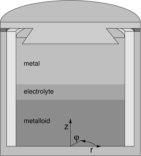
Figure 1: Conceptual design of a liquid metal self-assembling cell with coordinate system.

It goes without saying that the safe operation of such a cell requires the self-assembled layer structure of the three liquids to remain stable during charging and discharging.

For the quite similar case of aluminium reduction cells the interfacial instability is well known to set some lower limit for the thickness of the electrolyte below which the fluid starts to undergo a wavy motion that can ultimately interrupt the electrolysis. The same sort of instability has to be carefully considered for liquid batteries, too.

The focus of this paper is, however, on the existence of an upper limit of the size of the battery beyond which the Tayler instability would stir up the liquids.

3 The Tayler instability for the ideal fluid

The Tayler instability is well known in astrophysics where it had been first discussed by Vandakurov [8] and Tayler [7]. It can be considered as a limiting case of the kink-instability in plasma physics that sets in when the safety factor (basically the ratio of axial to azimuthal magnetic field) falls below some critical value.

For an ideal fluid, without any viscosity and resistivity, Tayler [7] had given the condition of stability of a purely azimuthal magnetic field $B_{\varphi}(r)$ with respect to non-axialsymmetric perturbations (proportional to $\exp{(i\varphi)}$) in the following form:

$$-\frac{d}{dr}(rB^{2}_{\varphi}(r))>0\;.$$ (1)

Despite its restriction to ideal fluids, which will be relaxed in the next section, it is worthwhile to analyze this expression a bit further. With view on our goal to avoid the TI in batteries, we will consider not only the obvious case of a completely filled cylindrical vessel with a homogeneous current distribution, but also the more general situation of a homogeneous current through the liquid in a hollow cylinder, together with an additional independent current along the axis.

Assume the fluid to fill the hollow cylinder between the inner radius $r_{\text{i}}$ and the outer radius $r_{\text{o}}$, with the ratio of the radii denoted by $\eta=r_{\text{i}}/r_{\text{o}}$. The current density $j$ through this cylindrical gap is assumed homogeneous so that the total current through the liquid is $I_{\text{f}}=\pi(r^{2}_{\text{o}}-r^{2}_{\text{i}})j$. Assume further the existence of an independent current $I_{\text{a}}$ along the central axis of the cylinder. Applied to liquid metal batteries, this scheme is depicted in Fig. 2.

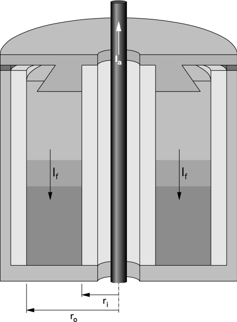
Figure 2: Sketch of a liquid metal battery with a central bore and a conductor for a stabilizing axial current.

Under these conditions the azimuthal magnetic field in the fluid acquires the form

$$B_{\varphi}(r)=\alpha r+\beta/r\;$$ (2)

with the constants $\alpha$ and $\beta$ given by

$$\alpha = \frac{\mu_{0}}{2\pi}\;\frac{I_{\text{f}}}{r^{2}_{\text{o}}}\;\frac{1}{1-\eta^{2}}\;,$$ (3)

$$\beta = \frac{\mu_{0}}{2\pi}\;\left[I_{\text{a}}-I_{\text{f}}\frac{\eta^{2}}{1-\eta^{2}}\right]\;.$$ (4)

The stability condition (1) can then be re-written in the form

$$\frac{\beta^{2}}{r^{2}}-2\alpha\beta-3\alpha^{2}r^{2}>0\;.$$ (5)

From the specific radial dependence of this expression it is evident that the most dangerous position for the instability to occur is close to $r_{\text{o}}$. Therefore, in order to identify the critical values for $\beta$, it is sufficient to solve the quadratic equation

$$\beta^{2}-2\alpha\beta r^{2}_{\text{o}}-3\alpha^{2}r^{4}_{\text{o}}=0\;.$$ (6)

only at $r_{\text{o}}$. This quadratic equation has two solutions which are $\beta_{1}=-ar^{2}_{\text{o}}$ and $\beta_{2}=3ar^{2}_{\text{o}}$. Expressed in terms of the current $I_{\text{a}}$ and $I_{\text{f}}$, this can be rewritten into the following two conditions for stability:

$$I_{\text{a}}<-I_{\text{f}}$$ (7)

or

$$I_{\text{a}}>I_{\text{f}}\frac{3+\eta^{2}}{1-\eta^{2}}\;.$$ (8)

These two inequalities are the main result of this section. They suggest two simple possibilities to avoid the TI. Either one applies $I_{\text{a}}$ in opposite direction to $I_{\text{f}}$: then $I_{\text{a}}$ has to be at least as strong as $I_{\text{f}}$. Or one applies $I_{\text{a}}$ in the same direction as $I_{\text{f}}$. Then $I_{\text{a}}$ has to be factor $(3+\eta^{2})/(1-\eta^{2})$ stronger than $I_{\text{f}}$.

This is illustrated in Fig. 3 where we show, for the particular case $\eta=0.5$, the (normalized) function $-rB^{2}_{\varphi}(r)$ for various values of $I_{\text{a}}/I_{\text{f}}$. For all curves with $-1<I_{\text{a}}/I_{\text{f}}<13/3$ we can identify regions (at least close to $r_{\text{o}}$) where the function $-rB^{2}_{\varphi}(r)$ has an outward decreasing part. Both for $I_{\text{a}}/I_{\text{f}}<-1$ and for $I_{\text{a}}/I_{\text{f}}>13/3$, however, the function $-rB^{2}_{\varphi}(r)$ increases monotonically.

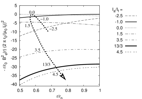
Figure 3: Dependence of the normalized function $-rB^{2}_{\varphi}(r)$ on the parameter $I_{\text{a}}/I_{\text{f}}$ for the particular case $\eta=0.5$. Note the monotonic increase of this function both for $I_{\text{a}}/I_{\text{f}}<-1$ and for $I_{\text{a}}/I_{\text{f}}>13/3$ which indicates the absence of the Tayler instability. The thick dashed line with an arrow indicates the change of the profiles when going from negative to positive $I_{\text{a}}/I_{\text{f}}$

For the purpose of batteries, the first version with $I_{\text{a}}<-I_{\text{f}}$ seems much more convenient. The limiting case $I_{\text{a}}=-I_{\text{f}}$ can be implemented by simply returning the battery current through the inner hole of the battery.

4 The Tayler instability for real fluids

While in case of an ideal fluid with a homogeneous current distribution the TI would set in already for arbitrary small currents, the main effect of finite viscosity and resistivity is to shift this threshold to some finite value.

In this section we will determine the critical currents for some real liquid metals which seem most important in our context, and we will study their dependence on the radii ratio $\eta$.

In the appendix we delineate the numerical scheme for the determination of the critical current which relies on the scheme outlined in [10, 11]. In this respect it is important to note that the relevant number here is the so-called Hartmann number $Ha=BR\sqrt{\sigma/(\rho\nu)}$, where $B$ is the magnetic field strength and $R$ is the radius of the cell. Hence, the larger the factor $\sqrt{\sigma/(\rho\nu)}$, the easier the TI will be excited for a given current. This means. in turn, that if we have a self-assembled layer of liquids, the most critical one of them is that with the highest factor. It turns out quickly that the typical metals (Mg, Na) forming the negative electrode are more prone to TI than the half-metals (Sb, Bi) forming the positive electrode.

In the following we will consider two of the most relevant materials. The first is Mg at 700^∘C with the parameters $\sigma=3.61\times 10^{6}$ S/m, $\rho=1.54\times 10^{3}$ kg/m³, $\nu=6.74\times 10^{-7}$ m²/s, the second is Na at 300^∘C with $\sigma=5.99\times 10^{6}$ S/m, $\rho=0.878\times 10^{3}$ kg/m³, $\nu=3.94\times 10^{-7}$ m²/s.

Figure 4: Critical current in dependence on $\eta$ for Mg at 700^∘C, under the assumption of a current density of 10 kA/m².

Let us assume now a current density of 10 kA/m² as it has been discussed as a typical achievable value for liquid metal batteries [1]. For Mg, the solid line in Fig. 4 shows the increasing dependence of the critical current on the ratio $r_{\text{i}}/r_{\text{o}}$. For $r_{\text{i}}/r_{\text{o}}=0$ the critical current is approximately 2 kA (note that this value is independent of the radius). This means, in turn, that the maximum area $\pi r^{2}_{\text{o}}$ (for the assumed current density of 10 kA/m²) is 0.2 m². If we would like to increase the bearable current we have to increase $r_{\text{i}}/r_{\text{o}}$. In this case, however, the total current through the cylindrical gap also decreases as $\sim(r^{2}_{\text{o}}-r^{2}_{\text{i}})$, which is depicted by the various non-solid curves in Fig. 4. At the crossing point between these curves with the solid curve one can identify the maximum current that would be possible for a given total area $\pi r^{2}_{\text{o}}$. For example, take the case of a rather large area $\pi r^{2}_{\text{o}}=2$ m². Evidently, for this case we cannot achieve an expected total current of 20 kA which would be a factor 10 higher than the critical current at $r_{\text{i}}/r_{\text{o}}=0$. Yet we can get a total current of around 12.5 kA, if we choose $r_{\text{i}}/r_{\text{o}}=0.61$.

Figure 5: Critical current in dependence on $\eta$ for Na at 300^∘C, under the assumption of a current density of 10 kA/m².

For sodium the situation is even more critical as shown in Fig. 5. Here, the current threshold at $r_{\text{i}}/r_{\text{o}}=0$ is approximately 0.86 kA, and even with an area $\pi r^{2}_{\text{o}}=1$ m² we can only achieve a critical current of 6.1 kA if we go to $r_{\text{i}}/r_{\text{o}}=0.62$

Note that the focus of this section was on identifying the threshold-increasing effect of hollow cylinders, without taking into account any (significant) axial current $I_{\text{a}}$. It is clear, however, that the idea of the former section to avoid the TI by sending an opposite directed current through the middle remains valid also in the case of real-world liquid metals.

5 Conclusion

The main purpose of this paper was to point out that the TI could represent a serious obstacle for the upward scalability of liquid metal batteries. If it occurred in one of the liquid layers (most likely in the upper metal, having the highest conductivity and the lowest density) it would lead to a vigorous motion and very likely to a mixing of the layers with possibly ”explosive” consequences. To give a first conservative estimate for the critical currents, we have used a simplified one-dimensional numerical model assuming an infinite ratio of height to the radius of a battery with pre-supposed cylindrical geometry. For any realistic aspect ratio, this estimate has to be concretized by appropriate two-dimensional simulations [12], which would give larger values of the critical currents. Another, although not a dramatic, modification of our results should be expected for the case that the shape of the battery is not a cylinder but, e.g., a cuboid.

We have also discussed two ways of how the TI can be avoided. One of them is the use of an inner non-conducting tube whose mere existence leads to a significant upward shift of the critical current. For a typical cell area in the order of 1 m² this might indeed represent a viable technical means for excluding TI. A more radical way that can be expected to suppress the TI completely is just to return the current through the hollow cylinder in the middle. The same effect could be achieved by applying a parallel axial current which is at least a factor $\frac{3+\eta^{2}}{1-\eta^{2}}$ as large as the current in the fluid.

Many theoretical aspects of the TI in liquid metal batteries are yet to be discussed. First experiments are presently carried out to study the TI in a cylindrical liquid metal and to validate various possible ways how it can be avoided.

Appendix A The mathematics of Tayler instability

In this appendix we describe how to determine the critical current of the TI for the hypothetical case of a cylinder with infinite length. For this purpose we use a simplified version of the procedure described in detail in [10]. We start with the Navier-Stokes equation for the velocity field $\bf{V}$

$$\frac{\partial{\bf V}}{\partial t}+({\bf V}\cdot{\bf\nabla}){\bf V} = -\frac{1}{\rho}{\bf\nabla}P+\nu\Delta{\bf V}+\frac{1}{\mu_{0}}({\bf\nabla}\times{\bf B})\times{\bf B}$$ (9)

and the induction equation for the magnetic field $\bf B$

$$\frac{\partial{\bf B}}{\partial t} = {\bf\nabla}\times({\bf V}\times{\bf B})+\frac{1}{\mu_{0}\sigma}\Delta{\bf B}\;.$$ (10)

Here, $\rho$ is the density of the fluid, $\nu$ its kinematic viscosity, $\sigma$ its electrical conductivity and $\mu_{0}$ the magnetic permeability of the free space. We also note that both fields have to be divergence-free (we assume incompressibility of the fluid):

$${\bf\nabla}\cdot{\bf V}=0,\;\;\;{\bf\nabla}\cdot{\bf B}=0\;.$$ (11)

Both ${\bf V}$ and ${\bf B}$, as well as the pressure $P$, are now split into the basic state and a perturbation according to

$${\bf V}={\bf V}_{0}+{\tilde{\bf v}}\;\;\;P=P_{0}+{\tilde{p}}\;\;\;{\bf B}={\bf B}_{0}+{\tilde{\bf b}}\;.$$ (12)

In our particular case the basic state of the velocity is just ${\bf V}_{0}=0$, while the basic state of the magnetic field is given by

$$B_{r,0}=0,\;\;\;B_{\varphi,0}(r)=\alpha r+\beta/r,\;\;\;B_{z,0}=0$$ (13)

with the constants $\alpha$ and $\beta$ given by

$$\alpha = \frac{\mu_{0}}{2\pi}\;\frac{I_{\text{f}}}{r^{2}_{\text{o}}}\;\frac{1}{1-\eta^{2}}$$ (14)

$$\beta = \frac{\mu_{0}}{2\pi}\;\left[I_{\text{a}}-I_{\text{f}}\frac{\eta^{2}}{1-\eta^{2}}\right]\;.$$ (15)

We employ now the usual normal mode analysis, by searching for solutions of the linearized equations for

$${\tilde{\bf v}}(r,\varphi,z,t)={\bf v}(r)\exp(i(kz+m\varphi+\omega t))$$ (16)

$${\tilde{p}}(r,\varphi,z,t)=p(r)\exp(i(kz+m\varphi+\omega t))$$ (17)

$${\tilde{\bf b}}(r,\varphi,z,t)={\bf b}(r)\exp(i(kz+m\varphi+\omega t))$$ (18)

This way, we end up with an eigenvalue system of ordinary differential equations (in $r$):

$$\frac{dv_{r}}{dr}+\frac{v_{r}}{r}+\frac{im}{r}v_{\varphi}+ikv_{z} = 0$$ (19)

$$\frac{dp}{dr}+i\frac{m}{r}X_{2}+ikX_{3}+\left(k^{2}+\frac{m^{2}}{r^{2}}\right)u_{r}$$

$$-i{\rm Ha_{\text{i}}}^{2}\frac{m}{r}B_{\varphi,0}b_{r}+2{\rm Ha_{\text{i}}}^{2}\frac{B_{\varphi}}{r}b_{\varphi} = 0$$ (20)

$$\frac{dX_{2}}{dr}-\left(k^{2}+\frac{m^{2}}{r^{2}}\right)v_{\varphi}+2i\frac{m}{r^{2}}v_{r}$$

$$+\frac{{\rm Ha_{\text{i}}}^{2}}{r}\frac{d}{dr}(rB_{\varphi,0})b_{r}+i{\rm Ha_{\text{i}}}^{2}\frac{m}{r}B_{\varphi,0}b_{\varphi}-i\frac{m}{r}p = 0$$ (21)

$$\frac{dX_{3}}{dr}+\frac{X_{3}}{r}-\left(k^{2}+\frac{m^{2}}{r^{2}}\right)v_{z}-ikp+i{\rm Ha_{\text{i}}}^{2}\frac{m}{r}B_{\varphi,0}b_{z} = 0$$ (22)

$$\frac{db_{r}}{dr}+\frac{b_{r}}{r}+\frac{im}{r}b_{\varphi}+ikb_{z} = 0$$ (23)

$$\frac{db_{z}}{dr}-\frac{i}{k}\left(k^{2}+\frac{m^{2}}{r^{2}}\right)b_{r}+\frac{m}{kr}X_{4}-\frac{m}{kr}B_{\varphi,0}u_{r} = 0$$ (24)

$$\frac{dX_{4}}{dr}-\left(k^{2}+\frac{m^{2}}{r^{2}}\right)b_{\varphi}+i\frac{2m}{r^{2}}b_{r}$$

$$-r\frac{d}{dr}\left(\frac{B_{\varphi,0}}{r}\right)v_{r}+i\frac{m}{r}B_{\varphi,0}v_{\varphi} = 0$$ (25)

where the abbreviations

$$X_{2}=\frac{dv_{\varphi}}{dr}+\frac{v_{\varphi}}{r},\;\;\;X_{3}=\frac{dv_{z}}{dr},\;\;\;X_{4}=\frac{db_{\varphi}}{dr}+\frac{b_{\varphi}}{r}\;\;\;$$ (26)

have been used. The governing parameter ${\rm Ha_{\text{i}}}$ here is the so-called Hartmann number, defined with the magnetic field at the inner radius according to

$${\rm Ha_{\text{i}}} = B_{\varphi}(r_{\text{i}})\sqrt{r_{\text{i}}(r_{\text{o}}-r_{\text{i}})}\sqrt{\sigma/(\rho\nu)}$$ (27)

$$= \frac{\mu_{0}I_{\text{a}}}{2\pi r_{\text{i}}}\sqrt{r_{\text{i}}(r_{\text{o}}-r_{\text{i}})}\sqrt{\sigma/(\rho\nu)}\;.$$ (28)

In the numerical implementation we will always use a (possibly very small) axial current. The boundary conditions, both at $r_{\text{i}}$ and $r_{\text{o}}$, for the velocity are the usual no-slip conditions

$$v_{r}=v_{\varphi}=v_{z}=0$$ (29)

As for the magnetic field, we assume insulating boundary conditions which can be written as

$$b_{\varphi}-\frac{m}{kr_{\text{i}}}b_{z} = 0$$ (30)

$$b_{r}+\frac{i}{I_{m}(kr_{\text{i}})}\left(\frac{m}{kr_{\text{i}}}I_{m}(kr_{\text{i}})-I_{m+1}(kr_{\text{i}}))\right)b_{z} = 0$$ (31)

at the inner boundary $r_{\text{i}}$ and

$$b_{\varphi}-\frac{m}{kr_{\text{o}}}b_{z} = 0$$ (32)

$$b_{r}+\frac{i}{K_{m}(kr_{\text{o}})}\left(\frac{m}{kr_{\text{o}}}K_{m}(kr_{\text{o}})-K_{m+1}(kr_{\text{o}}))\right)b_{z} = 0$$ (33)

at the outer boundary $r_{\text{o}}$. Note that $I_{m}$ and $K_{m}$ represent the modified Bessel functions.

In order to determine the critical currents for a given ratio of $\eta$ and $I_{\text{a}}/I_{\text{f}}$ we solve the above eigenvalue system by means of a shooting method adopted from [14]. Then we have to look for those wavenumbers $k$ that lead to a minimum critical $I_{\text{a}}$.

References

- [1] D. Sadoway, G. Ceder, D. Bradwell, High-amperage energy storage device and method, US Patent application, US 2008/0044725 A1, 2008.
- [2] D. Bradwell, Technical and economic feasibility of a high-temperature self-assembling battery, Master Thesis, MIT, 2006.
- [3] B. Agruss, Regenerative Battery, US Patent 3,245,836, 1966.
- [4] T. Oshima, M. Kajita, A. Okuno, Development of Sodium-Sulfur Batteries, Int J. Appl. Ceram. Techn. 1 (2004) 269-276.
- [5] T. Sele, Instabilities of the metal surfaces in electrolytic aluminum reduction cells, Met. Trans. B 8 (1977) 613-618.
- [6] P.A. Davidson, Overcoming instabilities in aluminium reduction cells: a route to cheaper aluminium, Mat. Sci. Technol. 16 (2000) 475-479.
- [7] R.J. Tayler, Adiabatic stability of stars containing magnetic fields. 1 – Toroidal fields, Mon. Not. R. Astron. Soc. 161 (1973) 365-380.
- [8] Y.V. Vandakurov, Theory for the stability of a star with a toroidal magnetic field, Sov. Astron. 16 (1972) 265-272.
- [9] W.F. Bergerson, C.B. Forest, G. Fiksel, D.A. Hannum, R. Kendrick, J.S. Sarff, S. Stambler, Onset and saturation of the kink instability in a current–carrying line-tied plasma, Phys. Rev. Lett. 96 (2006), 015004.
- [10] G. Rüdiger, M. Schultz, D. Shalybkov, R. Hollerbach, Theory of current–driven instability experiments in magnetic Taylor–Couette flows, Phys. Rev. E 76 (2007) 056309.
- [11] G. Rüdiger, M. Schultz, Tayler instability of toroidal magnetic fields in MHD Taylor-Couette flows, Astron. Nachr. 331 (2010), 121-129.
- [12] M. Gellert, G. Rüdiger, Eddy diffusivity from hydromagnetic Taylor–Couette flow experiments, Phys. Rev. E 80 (2009), 046314.
- [13] B. Agruss, H.B. Karas, The thermally regenerative liquid metal concentration cell, in: C.E. Crouthamel, H.L. Recht (Eds.), Regenerative EMF Cells, ACS, Washington, 1967, 62–81.
- [14] W.H. Press, S.A. Teukolsky, W.T. Vetterling, B.F. Flannery, Numerical Recipes, Cambridge University Press, Cambridge, 1992.