Color neutral 2SC phase of cold and dense quark matter in the presence of constant magnetic fields

Abstract

The color neutral two-flavor superconducting (2SC) phase of cold and dense quark matter is studied in the presence of constant magnetic fields and at moderate baryon densities. In the first part of the paper, a two-flavor effective Nambu–Jona-Lasinio (NJL) model consisting of a chiral symmetry breaking ($\chi$SB) mass gap $\sigma_{B}$, a color superconducting (CSC) mass gap $\Delta_{B}$ and a color chemical potential $\mu_{8}$ is introduced in the presence of a rotated $U(1)$ magnetic field $\tilde{\mathbf{B}}$. To study the phenomenon of magnetic catalysis in the presence of strong magnetic fields, the gap equations corresponding to $\sigma_{B}$ and $\Delta_{B}$, as well as $\mu_{8}$ are solved in the lowest Landau level (LLL) approximation. In the second part of the paper, a detailed numerical analysis is performed to explore the effect of any arbitrary magnetic field on the above mass gaps and the color chemical potential. The structure of the $\chi$SB and CSC phases is also presented in the $\mu_{c}-\tilde{e}B$ plane, and the effect of $\mu_{8}$ on the phase structure of the model is explored. As it turns out, whereas the transition from the $\chi$SB to CSC phase is of first order, nonvanishing $\mu_{8}$ affects essentially the second order phase transition from CSC to the normal phase.

I Introduction

Dense baryonic matter at low temperature and asymptotically large chemical potential is known to be a color superconductor old-CSC . This can be shown in the framework of perturbative Quantum Chromodynamics (pQCD). To explore the color superconducting phase at moderate chemical potential, however, it is necessary to use effective models, such as the well-known NJL model with four-fermion interaction NJL . Using an appropriate NJL type model, one can show that at baryon densities $\mu_{c}\simeq 350$ MeV, i.e. only several times larger than the density of nuclear matter, the two-flavor color superconducting (2SC) phase might be present shuryak ; huang2004 (see rajagopal2007 for recent reviews on color superconductivity in dense quark matter). Different astrophysical processes might therefore be influenced by the color superconductivity that is supposed to exist inside the compact stars. In ebert2005 , the competition between the chiral symmetry breaking and the color symmetry breaking condensates is investigated in the framework of a two-flavor color neutral NJL type model, including meson and diquark condensates, $\sigma_{0}$ and $\Delta_{0}$. Imposing the color neutrality condition, it is found that in the 2SC phase at $\mu>\mu_{c}=342$ MeV, the color chemical potential $\mu_{8}$ acquires rather small values of about $10$ MeV. Here, $\mu_{c}$ is the critical chemical potential. The diquark mass gap is numerically computed to be $\Delta_{0}\simeq 100$ MeV. It is also shown that the appearance of a coexistence regime (mixed phase) depends directly on the relative strength of the meson and diquark coupling constants $G_{S}$ and $G_{D}$. This is also indicated in berges1998 ; mixed ; huang2002 , where it is stated that neglecting the quark masses and choosing $G_{D}<G_{S}$, no mixed phase appears at $\mu>\mu_{c}$. The $\chi$SB and CSC phases can therefore be studied separately under these conditions.

In the present paper, we study the mesons and diquarks in the color neutral 2SC phase of cold and dense quark matter in the presence of constant magnetic fields. The aim is to study the effect of the magnetic field on the formation of chiral as well as diquark condensates, the dependence of mass gaps on the chemical potential $\mu$ and the external magnetic field, the phase diagram $\mu$ vs. $B$, and the effect of nonvanishing color chemical potential on the type of phase transitions for different $\mu$ and $B$ at zero temperature $T$.

The study of quark matter in the presence of constant magnetic field is relevant for the astrophysics of compact stars: Strong magnetic fields exist on the surface of compact stars. For neutron stars the magnetic fields $B\lesssim 10^{12}$ Gauß, whereas for magnetars, they can be as large as $B\simeq 10^{16}$ Gauß  thompson1996 . In the interiors of compact stars, the magnetic field can be even several orders of magnitude larger incera2010 . On the other hand, it is believed that the superdense interior of compact stars may be composed of electric and color neutral quark matter in the color superconducting phase. To test the predictions of astrophysical signatures of color superconductivity, a better understanding of the rôle of magnetic fields on the CSC phase is important. The study of superconducting phase in the presence of external magnetic fields is also relevant for the physics of heavy ion collisions: According to warringa ; kharzeev51-STAR , in off-central collisions, heavy ions possess a very large angular momentum and very strong magnetic fields can be created. In skokov , it is shown that the magnetic field presently created at RHIC is at most $eB\simeq 1.3\ m_{\pi}^{2}\sim 4.3\times 10^{18}$ Gauß, and the estimated value of the magnetic field strength for the LHC energy amounts to $15\ m_{\pi}^{2}\sim 5\times 10^{19}$ Gauß. Recently, the question of accessibility of the 2SC phase in the future heavy ion collision experiments is investigated in blaschke2010 . Here, the authors do not consider the effect of the before mentioned magnetic fields. It would be therefore important to study the effect of external magnetic fields on the formation of 2SC diquark condensates, as well as the corresponding phase structure in the presence of external magnetic fields. As for the results presented in this paper, they may be relevant only for the physics of the heavy ion collisions, because in contrary to the electric and color neutrality requirement of the superdense core of the compact stars, only the color neutrality condition is considered in this paper.

The effect of constant magnetic field on the formation of diquark condensates has been investigated by several authors. In rajagopal1999 ; gorbar2000 , it is shown that there is a linear combination of photon and a gluon that remains massless. The resulting “rotated” external magnetic field can therefore penetrate the color superconducting region without being affected by the Meissner effect. This has consequences for the structure of compact star cores. In ferrer2006 ; ferrer-CFL , the formation of magnetic color-flavor locked (MCFL) phase, as well as the transition to the paramagnetic-CFL (PCFL) phase are studied. In warringa2007 ; shovkovy2007 , it is shown that for small magnetic fields, the CFL mass gap as well as the corresponding magnetization exhibit small oscillations, the van Alfven–de Haas (vAdH) oscillations. This effect, which is well-known from condensed matter physics, is predicted by Landau and observed experimentally by van Alfven and de Haas (see alfven for an investigation of this effect in cold dense quark matter in a homogeneous magnetic field). The transport properties of 2SC phase is investigated recently in sedrakian2010 .

Recently, in mandal2009 , the formation of chiral and diquark condensates as well as their competition in the 2SC phase at zero temperature and moderate densities are studied using the same NJL type model as in the present paper. It is shown that for vanishing magnetic field, a mixed broken phase can be found where both chiral and superconducting gaps are non-zero. For $\tilde{e}B=0.05$ GeV² (corresponding to $B\simeq 8.5\times 10^{18}$ Gauß) and moderate diquark-to-chiral coupling ratios $G_{D}/G_{S}$, the chiral and superconducting transitions become weaker. For large $G_{D}/G_{S}$, strong magnetic fields disrupt the mixed broken phase region and a first order phase transition is found between the $\chi$SB and the CSC phase for $\tilde{e}B=0.05$ GeV². In contrast to mandal2009 , our results include a detailed analytical and numerical survey on the effect of external magnetic field and color chemical potential on cold and dense as well as color neutral quark matter in the presence of external magnetic fields.

The organization of this paper is as follows: In Sec. II, starting from an extended Lagrangian density of a gauged NJL model containing two flavors, and following the method presented in rajagopal1999 ; gorbar2000 , we introduce the rotated magnetic field $\tilde{e}B$ and determine the Lagrangian density containing the $\chi$SB and CSC mass gaps, $\sigma_{B}$ and $\Delta_{B}$, respectively. In Sec. III, the one-loop effective action and thermodynamic potential of the model are determined at zero temperature and finite quark chemical potential. In Sec. IV, assuming very strong magnetic fields, we solve analytically the gap equations corresponding to $\sigma_{B}$ and $\Delta_{B}$, as well as the color chemical potential $\mu_{8}$ in an appropriate LLL approximation. The $\chi$SB and the CSC phases are studied, in IV.A and IV.B, separately. This is possible because of our specific choice of free parameters, the quark mass $m_{0}$ and the meson and diquark couplings $G_{S}$ and $G_{D}$. In the $\chi$SB phase, characterized by $\sigma_{B}\neq 0$ and $\Delta_{B}=\mu_{8}=0$, the magnetic field enhances the bound state formation. This is because of the phenomenon of magnetic catalysis miransky1995 ; catalysis studied intensively in the past few years. In the CSC phase, characterized by $\sigma_{B}=0$, $\Delta_{B}\neq 0$ and $\mu_{8}\neq 0$, we determine analytically the $\mu$ and $\tilde{e}B$ dependence of $\Delta_{B}$ and $\mu_{8}$ in the regime of LLL dominance. In Sec. V, a numerical analysis is performed to study the $\tilde{e}B$ dependence of the $\chi$SB and CSC mass gaps at $\mu=250$ MeV (in the $\chi$SB regime) and $\mu=460$ MeV (in the CSC regime). For small values of $\tilde{e}B$, we observe vAdH oscillations in the mass gaps as well as the corresponding magnetizations, as expected. These are also observed in warringa2007 ; shovkovy2007 for three-flavor CFL phase at $\mu=500$ MeV. At $\tilde{e}B\simeq 0.45-0.5$ GeV², the oscillations end up in a “linear regime”. Comparing eventually our numerical results for $\tilde{e}B\gtrsim 0.45$ GeV² with the analytical results arising in Sec. IV for strong magnetic fields in the LLL approximation, we conclude that this approximation is only reliable in the above linear regime. The $\mu$-dependence of the mass gaps and the color chemical potential is also discussed for various $\tilde{e}B$. Our results for vanishing $\tilde{e}B$ coincide with the results in ebert2005 . We also present the phase structure of $\chi$SB and CSC phases in a $\mu_{c}-\tilde{e}B$ plane. In particular, we are interested on the effect of the color chemical potential $\mu_{8}$ on the phase structure of the model. As it turns out, for $\mu_{8}=0$, a first order phase transition exists between the $\chi$SB and the CSC phase in the regime $\mu_{c}\simeq 350-450$ MeV and $\tilde{e}B\in[0,0,7]$ GeV², whereas the transition from the CSC to the normal phase is of second order and occurs at $\mu_{c}\simeq 750-800$ MeV. For $\mu_{8}\neq 0$, however, whereas the phase transition between the $\chi$SB and the CSC phase is still of first order, the second order phase transition between the CSC and the normal phase goes over into a first order phase transition between the CSC and the normal phase at $\mu_{c}\simeq 755$ MeV and $\tilde{e}B\simeq 0.13$ GeV². Note that the first order nature of the transition between the $\chi$SB and CSC phases was expected from mandal2009 , where the type of phase transition between these two phases is studied for a fixed $\tilde{e}B=0.05$ GeV² and various $G_{D}/G_{S}$ ratios. Our results confirm the findings in mandal2009 for a wide range of $\tilde{e}B\in\{0,0.7\}$ GeV² and fixed value of $G_{D}/G_{S}=0.75$. Section VI is devoted to a summary of our results and concluding remarks.

II Two flavor 2SC model at $T=0$, and $\mu,B\neq 0$

Let us start with the fermionic part of the extended Lagrangian density of a gauged NJL model

$${\cal{L}}_{f}=\overline{\psi}(x)[i\gamma^{\mu}(\partial_{\mu}-ieQA_{\mu}-igT^{8}G^{8}_{\mu})-m_{0}+\hat{\mu}\gamma^{0}]\psi(x)$$ (II.1)

$$+G_{S}[(\overline{\psi}(x)\psi(x))^{2}+(\overline{\psi}(x)i\gamma_{5}\vec{\tau}\psi(x))^{2}]+G_{D}[(i\overline{\psi}^{C}(x)\epsilon_{f}\epsilon_{c}\gamma_{5}\psi(x))(i\overline{\psi}(x)\varepsilon_{f}\epsilon_{c}^{3}\gamma_{5}\psi^{C}(x))].$$

Here, $\psi^{C}=C\overline{\psi}^{T}$ and $\overline{\psi}^{C}=\psi^{T}C$ are charge-conjugate spinors, and $C=i\gamma^{2}\gamma^{0}$ is charge-conjugation matrix, $\vec{\tau}=(\tau_{1},\tau_{2},\tau_{3})$ are Pauli matrices. Moreover, $(\epsilon^{3}_{c})^{ab}\equiv(\epsilon_{c})^{ab3}$ and $(\varepsilon_{f})_{ij}$ are antisymmetric matrices in color and flavor spaces, respectively. For a theory with two quark flavors, $i,j=(1,2)=(u,d)$, and three color degrees of freedom $a,b=(1,2,3)=(r,g,b)$. We assume that both quarks have the same (bare) mass $m_{u}=m_{d}\equiv m_{0}$. Further, $\hat{\mu}$ is defined by $\hat{\mu}\equiv\mu+\sqrt{3}\mu_{8}\lambda_{8}$, where $\mu$ is the quark chemical potential and is responsible for the nonzero baryonic density of quark matter, and ${\mu}_{8}$ is inserted by hand to impose the color neutrality after the process of dynamical color symmetry breaking. Here, $T^{8}=\frac{\lambda_{8}}{2}$ with $\lambda_{8}=\frac{1}{\sqrt{3}}\mbox{diag}(1,1,-2)$ the $8^{\mbox{\small{th}}}$ Gell-Mann $\lambda$-matrix. The scalar and diquark couplings are denoted by $G_{S}$ and $G_{D}$, respectively. Furthermore, $Q=Q_{f}\otimes{\mathbf{1}}_{c}$ with $Q_{f}\equiv\mbox{diag}\left(2/3,-1/3\right)$ is the fermionic charge matrix coupled to $U(1)$ gauge field $A_{\mu}$. The same setup without the coupling to $A_{\mu}$ and $G_{\mu}^{8}$ is also used in ebert2005 . To determine the effective action of the above model, we introduce first the bosonized Lagrangian density

$${\cal{L}}_{f} = \overline{\psi}(x)[i\gamma^{\mu}(\partial_{\mu}-ieQA_{\mu}-igT^{8}G^{8}_{\mu})+\hat{\mu}\gamma^{0}]\psi(x)-\overline{\psi}(x)(m+i\gamma^{5}\vec{\tau}\cdot\vec{\pi})\psi(x)$$ (II.2)

$$-\frac{1}{2}\Delta^{*3}(i\overline{\psi}^{C}(x)\varepsilon_{f}\epsilon_{c}^{3}\gamma_{5}\psi(x))-\frac{1}{2}\Delta^{3}(i\overline{\psi}(x)\varepsilon_{f}\epsilon_{c}^{3}\gamma_{5}\psi^{C}(x))-\frac{\sigma^{2}+\vec{\pi}^{2}}{4G_{S}}-\frac{\Delta^{3}\Delta^{*3}}{4G_{D}},$$

with $m\equiv m_{0}+\sigma$, that includes the auxiliary mesonic fields

$$\sigma=-2G_{S}(\overline{\psi}\psi),\qquad\qquad\vec{\pi}=-2G_{S}(\overline{\psi}i\gamma^{5}\vec{\tau}\psi),$$ (II.3)

and diquarks

$$\Delta^{3}=-2G_{D}(i\overline{\psi}^{C}\varepsilon_{f}\epsilon_{c}^{3}\gamma_{5}\psi),\qquad\qquad\Delta^{*3}=-2G_{D}(i\overline{\psi}\varepsilon_{f}\epsilon_{c}^{3}\gamma_{5}\psi^{C}).$$ (II.4)

From now on, we will skip the supperscript “3” for $\Delta$ and $\Delta^{*}$. Using an appropriate mean field approximation, the effective potential of this model can be determined as a function of the condensates $\langle\sigma\rangle$, $\langle\vec{\pi}\rangle$,$\langle\Delta\rangle$ and $\langle\Delta^{*}\rangle$. For simplicity we set $\langle\vec{\pi}\rangle=\vec{0}$. It is the purpose of this paper to study the effect of a constant background $U(1)$ magnetic field on the formation of these condensates. To do this, we have, principally, to replace $A_{\mu}$ by a classical $A_{\mu}^{ext}$ and a dynamical part $a_{\mu}$ and then integrate out the dynamical gauge field $a_{\mu}$ and $G_{\mu}^{8}$. However, it turns out that for non-vanishing $(\Delta,\Delta^{*})$, both gauge fields $A_{\mu}$ and $G_{\mu}^{8}$ are massive and underlie the Meissner effect. They are therefore unappropriate to be taken as external fields. But, as it is shown in rajagopal1999 ; gorbar2000 , there is indeed a linear combination of $A_{\mu}$ and $G_{\mu}^{8}$, that leads to a massless “rotated” $U(1)$ field, $\tilde{A}_{\mu}=A_{\mu}\cos\theta-G_{\mu}^{8}\sin\theta$, and a massive “rotated” $SU(3)$ field, $\tilde{G}_{\mu}^{8}=A_{\mu}\sin\theta+G_{\mu}^{8}\cos\theta$. According to gorbar2000 , the angle $\theta$ can be determined from

$$\cos\theta\equiv-\frac{\sqrt{3}g}{\sqrt{3g^{2}+e^{2}}},\qquad\mbox{and}\qquad\sin\theta\equiv-\frac{e}{\sqrt{3g^{2}+e^{2}}}.$$ (II.5)

To rotate the fields, one uses the identity

$$eQA_{\mu}+gT^{8}G^{8}_{\mu}\equiv\tilde{e}\tilde{Q}\tilde{A}_{\mu}+\tilde{g}\tilde{T}\tilde{G}^{8}_{\mu},$$ (II.6)

and insert the combination ${\cal{O}}{\cal{O}}^{T}=1$ on the right hand side (r.h.s.) of this identity. Here, ${\cal{O}}$ is an appropriate rotation matrix including sine and cosine of $\theta$. The identity (II.6) not only determines the new rotated fields as a linear combination of the original non-rotated ones, it also fixes the relation between the rotated and non-rotated couplings as $\tilde{e}\tilde{Q}=eQ\cos\theta-gT^{8}\sin\theta$, as well as $\tilde{g}\tilde{T}=eQ\sin\theta+gT^{8}\cos\theta$. In the rotated system, one chooses $\tilde{Q}$ so that $\tilde{Q}\langle\Delta\rangle=0$. This leads to

$$\tilde{Q}=Q_{f}\otimes{\mathbf{1}}_{c}-{\mathbf{1}}_{f}\otimes(\frac{T^{8}}{\sqrt{3}})_{c}.$$ (II.7)

The above relations between the rotated and non-rotated generators, $(Q,T^{8})$ and $(\tilde{Q},\tilde{T})$, lead then to $\tilde{T}\langle\Delta\rangle\neq 0$, which then yields a non-vanishing mass for $\tilde{G}_{\mu}^{8}$. Hence, as long as the diquark condensate $\Delta$ is non-vanishing, the rotated $\tilde{G}_{\mu}^{8}$ is massive because of $\tilde{T}\langle\Delta\rangle\neq 0$. In this case, the rotated system is the true physical system. Once $\Delta=0$ and $\sigma\neq 0$, the rotated and non-rotated systems are equivalent, because the identity $\tilde{Q}\langle\sigma\rangle=\tilde{T}\langle\sigma\rangle=0$ holds automatically [see footnote 8]. Using (II.7) and the above relation $\tilde{e}\tilde{Q}=eQ\cos\theta-gT^{8}\sin\theta$ between the rotated $\tilde{e}\tilde{Q}$ and the non-rotated $eQ$, it turns out that $\tilde{e}\equiv e\cos\theta$, as in the electroweak Standard Model. In the six dimensional flavor-color representation, $(u_{r},u_{g},u_{b},d_{r},d_{g},d_{b})$, the rotated $\tilde{Q}$ charges of different quarks, in units of $\tilde{e}$, are presented in Table I.

quarks	$u_{r}$	$u_{g}$	$u_{b}$	$d_{r}$	$d_{g}$	$d_{b}$
$\tilde{q}$	$+\frac{1}{2}$	$+\frac{1}{2}$	1	$-\frac{1}{2}$	$-\frac{1}{2}$	0

Table 1: $\tilde{Q}$ charges of quarks in 2SC model in the presence of rotated magnetic field $\tilde{\mathbf{B}}$ in units of $\tilde{e}$.

Plugging (II.6) in (II.2), the resulting transformed Lagrangian density is then given by (II.2) with $eQA_{\mu}+gT^{8}G^{8}_{\mu}$ replaced by $\tilde{e}\tilde{Q}\tilde{A}_{\mu}+\tilde{g}\tilde{T}\tilde{G}^{8}_{\mu}$, and $\vec{\pi}=\vec{0}$ [see (II.6)], and reads

$${\cal{L}}_{f} = \overline{\psi}(x)[i\gamma^{\mu}(\partial_{\mu}-i\tilde{e}\tilde{Q}\tilde{A}_{\mu}-i\tilde{g}\tilde{T}\tilde{G}_{\mu}^{8})+\hat{\mu}\gamma^{0}]\psi(x)-m\overline{\psi}(x)\psi(x)$$ (II.8)

$$-\frac{1}{2}\Delta^{*}(i\overline{\psi}^{C}(x)\varepsilon_{f}\epsilon_{c}^{3}\gamma_{5}\psi(x))-\frac{1}{2}\Delta(i\overline{\psi}(x)\varepsilon_{f}\epsilon_{c}^{3}\gamma_{5}\psi^{C}(x))-\frac{\sigma^{2}}{4G_{S}}-\frac{|\Delta|^{2}}{4G_{D}},$$

with $|\Delta|^{2}\equiv\Delta\Delta^{*}$. To introduce the external rotated $U(1)$ magnetic field in the third direction, we replace $\tilde{A}_{\mu}\to\tilde{A}_{\mu}^{ext}+\tilde{a}_{\mu}$, with the external rotated electromagnetic field $\tilde{A}_{\mu}^{ext}$ in the Landau gauge $\tilde{A}_{\mu}^{ext}=(0,0,Bx,0)$, and integrate out the remaining dynamical rotated fields $\tilde{a}_{\mu}$ and $\tilde{G}_{\mu}^{8}$. We arrive therefore at the full modified bosonized Lagrangian $\tilde{\cal{L}}=\tilde{\cal{L}}_{k}+\tilde{\cal{L}}_{f}$, with

$$\tilde{\cal{L}}_{k}\equiv-\left(\frac{\sigma^{2}}{4G_{S}}+\frac{|\Delta|^{2}}{4G_{D}}+\frac{B^{2}}{2}\right),$$ (II.9)

and

$$\tilde{\cal{L}}_{f} = \overline{\psi}(x)[i\gamma^{\mu}(\partial_{\mu}-i\tilde{e}\tilde{Q}\tilde{A}_{\mu}^{ext})+\hat{\mu}\gamma^{0}]\psi(x)-m\overline{\psi}(x)\psi(x)$$ (II.10)

$$-\frac{1}{2}\Delta^{*}(i\overline{\psi}^{C}(x)\varepsilon_{f}\epsilon^{3}_{c}\gamma_{5}\psi(x))-\frac{1}{2}\Delta(i\overline{\psi}(x)\varepsilon_{f}\epsilon^{3}_{c}\gamma_{5}\psi^{C}(x)),$$

in a constant (rotated) background $U(1)$ magnetic field $\tilde{\mathbf{B}}=B{\mathbf{e}}_{3}$. In what follows, we will simplify (II.10) using the method presented in ferrer2006 and arrive at an equivalent Lagrangian, which will then be used in Sec. III to determine the effective potential of the above model in the presence of a rotated background $U(1)$ magnetic field $\tilde{\mathbf{B}}$. To do this, we introduce the rotated-charge projectors $\Omega_{\tilde{q}}$, that satisfy the eigenvalue equation $\tilde{Q}\Omega_{\tilde{q}}=\tilde{q}\Omega_{\tilde{q}}$. They are given by

$$\begin{array}[]{lcrclcr}\Omega_{0}&=&\mbox{diag}(0,0,0,0,0,1),&&\Omega_{+\frac{1}{2}}&=&\mbox{diag}(1,1,0,0,0,0)\\ \Omega_{1}&=&\mbox{diag}(0,0,1,0,0,0),&&\Omega_{-\frac{1}{2}}&=&\mbox{diag}(0,0,0,1,1,0),\\ \end{array}$$

and satisfy

$$\sum_{\tilde{q}\in\{0,1,\pm\frac{1}{2}\}}\Omega_{\tilde{q}}=1,\qquad\mbox{and}\qquad\Omega_{\tilde{q}}\Omega_{{\tilde{q}}^{\prime}}=\delta_{\tilde{q}{\tilde{q}}^{\prime}}.$$ (II.12)

Using the definition $\psi_{\tilde{q}}(x)\equiv\Omega_{\tilde{q}}\psi(x)$, the fermion field in the six dimensional color-flavor representation can now given by

$$\psi=\sum_{\tilde{q}\in\{0,1,\pm\frac{1}{2}\}}\psi_{\tilde{q}}.$$ (II.13)

Introducing, at this stage, the Nambu-Gorkov bispinor wave function

$$\Psi_{\tilde{q}}=\left(\begin{array}[]{c}\psi_{\tilde{q}}\\ \psi^{C}_{-\tilde{q}}\end{array}\right),$$

the part of the Lagrangian which is bilinear in $\psi$, i.e. $\tilde{\cal{L}}_{f}$ from (II.10), can be brought in the following form:

$$\tilde{\cal{L}}_{f}=\frac{1}{2}\sum_{\tilde{q}\in\{0,1,\pm\frac{1}{2}\}}\overline{\Psi}_{\tilde{q}}(x){\cal{S}}_{\tilde{q}}{\Psi}_{\tilde{q}}(x),$$ (II.14)

where ${\cal{S}}_{\tilde{q}}$ for $\tilde{q}\in\{0,1\}$ is given by

$${\cal{S}}_{\tilde{q}\in\{0,1\}}\equiv\left(\begin{array}[]{cc}[G^{+}_{(\tilde{q})}]^{-1}&0\\ 0&[G^{-}_{(\tilde{q})}]^{-1}\\ \end{array}\right),$$ (II.17)

and for $\tilde{q}\in\{-\frac{1}{2},+\frac{1}{2}\}$ by

$${\cal{S}}_{\tilde{q}\in\{-\frac{1}{2},+\frac{1}{2}\}}\equiv\left(\begin{array}[]{cc}[G^{+}_{(\tilde{q})}]^{-1}&-\kappa\Omega_{-\tilde{q}}\\ -\kappa^{\prime}\Omega_{\tilde{q}}&[G^{-}_{(\tilde{q})}]^{-1}\\ \end{array}\right).$$ (II.20)

Here, $[G^{\pm}_{(\tilde{q})}]^{-1}\equiv[\gamma^{\mu}(i\partial_{\mu}+\tilde{e}\tilde{q}\tilde{A}_{\mu}\pm\hat{\mu}\delta_{\mu 0})-m],$ and $\kappa^{ij,ab}_{\alpha\beta}\equiv i\Delta\tau_{2}^{ij}\lambda_{2}^{ab}\gamma^{5}_{\alpha\beta}$ as well as $\kappa^{\prime}\equiv\gamma_{0}\kappa^{\dagger}\gamma_{0}=i\Delta^{*}\tau_{2}\lambda_{2}\gamma^{5}$. They can be read from (II.10) and the relations (II.12) as well as the definition of $\psi_{\tilde{q}}=\Omega_{\tilde{q}}\psi$. Note that (II.14) can be equivalently expressed as

$$\tilde{\cal{L}}_{f} = \frac{1}{2}\sum_{\tilde{q}\in\{0,1,\pm\frac{1}{2}\}}\bigg{\{}\overline{\psi}^{C}_{\tilde{q}}(x)[G^{-}_{(-\tilde{q})}]^{-1}\psi^{C}_{\tilde{q}}(x)+\overline{\psi}_{\tilde{q}}(x)[G^{+}_{(\tilde{q})}]^{-1}\psi_{\tilde{q}}(x)-\overline{\psi}_{\tilde{q}}^{C}(x)\tilde{\kappa}^{\prime}_{\tilde{q}}\psi_{\tilde{q}}(x)-\overline{\psi}_{\tilde{q}}(x)\tilde{\kappa}_{\tilde{q}}\psi_{\tilde{q}}^{C}(x)\bigg{\}},$$

where, $\tilde{\kappa}_{\tilde{q}}$ is defined by $\tilde{\kappa}_{\tilde{q}}\equiv\Omega_{\tilde{q}^{\prime}}\kappa\Omega_{\tilde{q}}$. In (II), $\tilde{\kappa}_{\tilde{q}}$ is non-vanishing only for $\tilde{q}^{\prime}+\tilde{q}=0$ with $\tilde{q}^{\prime}\neq\tilde{q}$. For $\tilde{q}\in\{-\frac{1}{2},+\frac{1}{2}\}$ we have therefore

$$(\tilde{\kappa}_{\tilde{q}=-\frac{1}{2}})_{\rho\sigma}=(\Omega_{\frac{1}{2}}\kappa\Omega_{-\frac{1}{2}})_{\rho\sigma} = (\kappa\Omega_{-\frac{1}{2}})_{\rho\sigma}=\left\{\begin{array}[]{ccrcl}+i\Delta\gamma^{5}&\mbox{if}&(\rho,\sigma)&=&(2,4),\\ -i\Delta\gamma^{5}&\mbox{if}&(\rho,\sigma)&=&(1,5),\\ 0&\mbox{otherwise},&&&\end{array}\right.$$ (II.25)

$$(\tilde{\kappa}_{\tilde{q}=+\frac{1}{2}})_{\rho\sigma}=(\Omega_{-\frac{1}{2}}\kappa\Omega_{\frac{1}{2}})_{\rho\sigma} = (\kappa\Omega_{+\frac{1}{2}})_{\rho\sigma}=\left\{\begin{array}[]{ccrcl}+i\Delta\gamma^{5}&\mbox{if}&(\rho,\sigma)&=&(4,2),\\ -i\Delta\gamma^{5}&\mbox{if}&(\rho,\sigma)&=&(5,1),\\ 0&\mbox{otherwise},\end{array}\right.$$ (II.29)

whereas for $\tilde{q}\in\{0,1\}$, we have

$$\tilde{\kappa}_{ij}=(\Omega_{i}\kappa\Omega_{j})_{\rho\sigma} = 0,\qquad\mbox{for}\qquad i,j=0,1\qquad\mbox{or}\qquad i=j=\pm\frac{1}{2}.$$ (II.30)

This is in contrast to the case of three-flavor color-flavor locked (CFL) phase, studied in ferrer2006 . In that case, there exists a charge $\tilde{q}=-1$ and the combination of $(\Omega_{\mp 1}\kappa\Omega_{\pm 1})$ leads also to nonzero result.

III One-loop effective action and thermodynamic potential

In what follows, the one-loop effective action of the theory, $\Gamma$, will be determined in the mean field approximation in terms of $\sigma\equiv\langle\sigma(x)\rangle,\Delta\equiv\langle\Delta(x)\rangle$, and $\Delta^{*}\equiv\langle\Delta^{*}(x)\rangle$. Using the following path integral over the quark fields

$$e^{i\Gamma[\sigma,\Delta,\Delta^{*}]}=\int{\cal{D}}\psi{\cal{D}}\bar{\psi}\exp\left(i\int d^{4}x~{}\tilde{\cal{L}}\right),$$ (III.1)

where, $\tilde{\cal{L}}\equiv\tilde{\cal{L}}_{k}+\tilde{\cal{L}}_{f}$, with $\tilde{\cal{L}}_{k}$ and $\tilde{\cal{L}}_{f}$ from (II.9) and (II.14), the effective action up to one-loop quantum corrections is given by

$$\Gamma[\sigma,\Delta,\Delta^{*}]=-\left(\frac{\sigma^{2}}{4G_{S}}+\frac{|\Delta|^{2}}{4G_{D}}+\frac{B^{2}}{2}\right){\cal{V}}+\Gamma_{\mbox{\tiny{eff}}}^{(1)}[\sigma,\Delta,\Delta^{*}].$$ (III.2)

Here, ${\cal{V}}$ is the 4-dimensional space-time volume, and $\Gamma_{\mbox{\tiny{eff}}}^{(1)}$ is the one-loop contribution to the effective potential. It arises by integrating out the fermion fields and reads

$$\Gamma^{(1)}_{\mbox{\tiny{eff}}}=-\frac{i}{2}\sum_{\tilde{q}}{\mbox{Tr}}_{\{NGcfsx\}}~{}\ln[{{\cal{S}}_{\tilde{q}}}^{-1}],$$ (III.3)

where ${\cal{S}}_{\tilde{q}}$ is defined in (II.17) and (II.20). Here, the trace “Tr” operation in (III.3) includes apart from a two-dimensional trace in the Nambu-Gorkov (NG) space, a trace over the whole phase space. It is therefore defined by a trace over the color ($c$), flavor ($f$), and spinor ($s$) degrees of freedom, as well as over a four-dimensional space-time coordinate ($x$) ebert2005 . To compute (III.3), we have to notice that, according to Table 1, the blue quarks $(u_{b},d_{b})$ have $\tilde{q}=0,1$, whereas the green and red quarks $(u_{r},u_{g},d_{r},d_{g})$ have $\tilde{q}=\pm\frac{1}{2}$. Thus relation (III.3) reduces to

$$\Gamma^{(1)}_{\mbox{\tiny{eff}}}=\sum\limits_{\kappa\in\{r,g,b\}}\Gamma^{(1)/\kappa}_{\mbox{\tiny{eff}}},$$ (III.4)

where the one-loop effective action of the blue (b) and red/green (r/g) are given by

$$\Gamma^{(1)/\mbox{\tiny{b}}}_{\mbox{\tiny{eff}}} = -\frac{i}{2}\mbox{Tr}_{\{NGcfsx\}}\ln[{{\cal{S}}_{0}}^{-1}]-\frac{i}{2}\mbox{Tr}_{\{NGcfsx\}}\ln[{{\cal{S}}_{+1}}^{-1}],$$

$$\sum\limits_{\kappa\in\{r,g\}}\Gamma^{(1)/\kappa}_{\mbox{\tiny{eff}}} = -\frac{i}{2}\mbox{Tr}_{\{NGcfsx\}}\ln[{{\cal{S}}_{+\frac{1}{2}}}^{-1}]-\frac{i}{2}\mbox{Tr}_{\{NGcfsx\}}\ln[{{\cal{S}}_{-\frac{1}{2}}}^{-1}].$$ (III.5)

To perform the trace operation in the NG space, we use

$$\det\left(\begin{array}[]{rr}A&B\\ C&D\\ \end{array}\right)=\det\left(-BC+BDB^{-1}A\right)=\det\left(-CB+CAC^{-1}D\right).$$ (III.8)

Using further $\mbox{tr}\ln A=\ln\det A$, we arrive at

$${\det}_{\{NGcfsx\}}[{{\cal{S}}_{0}}^{-1}] = {\det}_{\{scx\}}\big{[}\{\gamma^{\alpha}(i\partial_{\alpha}+\breve{\mu}\delta_{\alpha 0})-m\}\{\gamma^{\alpha}(i\partial_{\alpha}-\breve{\mu}\delta_{\alpha 0})-m\}\big{]},$$

$${\det}_{\{NGcfsx\}}[{{\cal{S}}_{+1}}^{-1}] = {\det}_{\{scx\}}\big{[}\{\gamma^{\alpha}(i\partial_{\alpha}+\tilde{e}\tilde{A}_{\alpha}+\breve{\mu}\delta_{\alpha 0})-m\}\{\gamma^{\alpha}(i\partial_{\alpha}+\tilde{e}\tilde{A}_{\alpha}-\breve{\mu}\delta_{\alpha 0})-m\}\big{]},$$

$${\det}_{\{NGcfsx\}}[{{\cal{S}}_{\pm\frac{1}{2}}}^{-1}] = {\det}_{\{scx\}}\big{[}|\Delta|^{2}+\{-\gamma^{\alpha}(i\partial_{\alpha}\pm\frac{1}{2}\tilde{e}\tilde{A}_{\alpha}+\bar{\mu}\delta_{\alpha 0})-m\}$$ (III.9)

$$\qquad\qquad\times\{\gamma^{\alpha}(i\partial_{\alpha}\pm\frac{1}{2}\tilde{e}\tilde{A}_{\alpha}-\bar{\mu}\delta_{\alpha 0})-m\}\big{]},$$

where we have skipped the superscript “ext” on the external rotated gauge field $\tilde{A}_{\mu}$. Here, $\breve{\mu}\equiv\mu-2\mu_{8}$, $\bar{\mu}\equiv\mu+\mu_{8}$ and $m\equiv m_{0}+\sigma$. The determinants in (III) are now to be calculated in the momentum space. To do this, a generalization of the method described in ferrer2006 for arbitrary charges is necessary. This method is originally developed by Ritus in ritus1972 in order to determine the Green’s function of charged fermions in the presence of background magnetic field. It is then extended to charged vector fields in elizalde2004 . Recently, it is used in fukushima2009 to determine the electric-current susceptibility of quark matter in the presence of external constant magnetic field. As it is described in fukushima2009 , in the Landau gauge for the external rotated gauge field, a projection operator $P_{n}$ can be defined

$$\begin{array}[]{rclccc}P_{n}&\equiv&\frac{1}{2}[f_{n_{+}}(x)+f_{n_{-}}(x)]+\frac{i}{2}[f_{n_{+}}(x)-f_{n_{-}}(x)]\gamma^{1}\gamma^{2},&&\mbox{for}&{q}B>0,\\ P_{n}&\equiv&\frac{1}{2}[f_{n_{+}}(x)+f_{n_{-}}(x)]-\frac{i}{2}[f_{n_{+}}(x)-f_{n_{-}}(x)]\gamma^{1}\gamma^{2},&&\mbox{for}&{q}B<0,\\ \end{array}$$ (III.12)

that includes the basis functions $f_{n_{\pm}}(x)$ defined by

$$\begin{array}[]{rclcrcl}f_{n_{+}}(x)&=&\phi_{n}(x-\frac{p_{y}}{{q}B}),&&n&=&0,1,2,\cdots,\\ f_{n_{-}}(x)&=&\phi_{n-1}(x-\frac{p_{y}}{{q}B}),&&n&=&1,2,3\cdots.\end{array}$$ (III.15)

Here, $\phi_{n}(x)$ are the standard Landau quantized wave functions fukushima2009

$$\phi_{n}(x)=\sqrt{\frac{1}{2^{n}n!}}\left(\frac{|{q}B|}{\pi}\right)^{1/4}\exp\left(-\frac{1}{2}|{q}B|x^{2}\right)H_{n}\left(\sqrt{|{q}B|}x\right),$$ (III.16)

with $H_{n}(x)$ the Hermite polynomial of degree $n$. Using the projectors $P_{n}$ from (III.12), it is easy to show that

$$\gamma_{\mu}\left(i\partial^{\mu}+{q}A^{\mu}\right)P_{n}e^{-i(p_{0}t-p_{y}y-p_{z}z)}=P_{n}\left(p_{0}\gamma^{0}-\mbox{sgn}({q}B)\sqrt{2|{q}B|n}\gamma^{2}-p_{z}\gamma^{3}\right)e^{-i(p_{0}t-p_{y}y-p_{z}z)}.$$

The r.h.s. of (III) is a free Dirac operator with a modified momentum

$$\bar{p}^{\mu}=(p_{0},0,\mbox{sgn}(qB)\sqrt{2|qB|n},p_{3}).$$ (III.18)

This shows also that the solution of the Dirac equation in the presence of a constant magnetic field can be given by a combination of the projection operators $P_{n}$ and the ordinary free Dirac spinors $u(p,s)$ and $v(p,s)$ fukushima2009 .

To compute the determinants in (III) in the momentum space, we will use, for the charges $\tilde{q}\neq 0$, an appropriate momentum basis, similar to (III.18), and for $\tilde{q}=0$, the ordinary four-momentum $p^{\mu}$. In other words, we have

$$\begin{array}[]{rclccrcl}{\bar{p}}_{\tilde{q}\neq 0}^{\mu}&=&(p_{0},0,\frac{\tilde{q}}{|\tilde{q}|}\sqrt{2|\tilde{q}\tilde{e}B|n},p_{3}),&&\mbox{for}&{\tilde{q}}&=&1,\pm\frac{1}{2},\\ {\bar{p}}_{\tilde{q}=0}^{\mu}&=&(p_{0},p_{1},p_{2},p_{3}),&&\mbox{for}&\tilde{q}&=&0,\end{array}$$ (III.21)

where $\frac{\tilde{q}}{|\tilde{q}|}$ replaces $\mbox{sgn}(\tilde{q}B)$ in (III.18). This leads to the well-known quasiparticle dispersion relations in the presence of a constant magnetic field aligned in the third direction shovkovy2007 ,

$$\begin{array}[]{rclccrcl}E_{\tilde{q}}&=&\sqrt{2|\tilde{q}\tilde{e}B|n+p_{3}^{2}+m^{2}}&&\mbox{for}&{\tilde{q}}&=&1,\pm\frac{1}{2},\\ E_{0}&=&\sqrt{p_{1}^{2}+p_{2}^{2}+p_{3}^{2}+m^{2}}&&\mbox{for}&{\tilde{q}}&=&0.\\ \end{array}$$ (III.24)

Using the momenta (III.21) and transforming (III.4) and (III) into the Fourier space, the one-loop effective action reads

$$\tilde{\Gamma}^{(1)}_{\mbox{\tiny{eff}}}(\bar{p})=\sum\limits_{\kappa\in\{r,g,b\}}\tilde{\Gamma}^{(1)/\kappa}_{\mbox{\tiny{eff}}}(\bar{p}),$$ (III.25)

with

$$\tilde{\Gamma}^{(1)/\mbox{\tiny{b}}}_{\mbox{\tiny{eff}}}(\bar{p}) = -i\sum\limits_{\tilde{q}\in\{0,1\}}\ln{\det}_{x}[\{({E}_{\tilde{q}}+\breve{\mu})^{2}-p_{0}^{2}\}\{({E}_{\tilde{q}}-\breve{\mu})^{2}-p_{0}^{2}\}],$$

$$\sum\limits_{\kappa\in\{r,g\}}\tilde{\Gamma}^{(1)/\kappa}_{\mbox{\tiny{eff}}}(\bar{p}) = -2i\sum\limits_{\tilde{q}\in\{+\frac{1}{2},-\frac{1}{2}\}}\ln{\det}_{x}[({{E}^{(+)}_{\tilde{q}}}^{2}-{p}_{0}^{2})({{E}^{(-)}_{\tilde{q}}}^{2}-{p}_{0}^{2})].$$ (III.26)

Here, $E_{\tilde{q}}$ for $\tilde{q}\in\{0,1,\pm\frac{1}{2}\}$ are defined in (III.24), and ${E}_{\tilde{q}}^{(\pm)}\equiv\sqrt{{(E_{\tilde{q}}\pm\bar{\mu})}^{2}+{|\Delta|}^{2}}$, for $\tilde{q}\in\{+\frac{1}{2},-\frac{1}{2}\}$. The factor 2 in the last equation of (III) reflects the degeneracy in the quark charges for $u_{r/g}$ as well as $d_{r/g}$ (see Table 1). Note that a trace over Landau levels, $n$, is implemented in the expression on the r.h.s. of (III). This is because $E_{\tilde{q}\neq 0}$ from (III.24) depends explicitly on $n$. This trace will be performed in the next step, where the one-loop effective action will be explicitly determined in the momentum space. Performing the remaining determinant in the coordinate space leads, for a constant background magnetic field, to a space-time volume ${\cal{V}}$. At this stage, we will introduce the effective thermodynamic (mean field) potential $\Omega_{\mbox{\tiny{eff}}}$, that is defined by the effective action through the relation $\Gamma_{\mbox{\tiny{eff}}}=-{\cal{V}}\Omega_{\mbox{\tiny{eff}}}$. To determine the one-loop contribution to the one-loop effective potential at zero temperature $\Omega_{\mbox{\tiny{eff}}}^{(1)}$, it is convenient to determine it first at finite temperature, and then taking the limit $T\to 0$, consider only the zero temperature effects shovkovy2007 . For quarks with $\tilde{q}=0$, one replaces $p_{0}$ by $p_{0}=i\omega_{\ell}$, where $\omega_{\ell}$ are the Matsubara frequency defined by $\omega_{\ell}\equiv(2\ell+1)\pi T$, and the $p_{0}$ integration by an infinite sum over the Matsubara frequencies. For an arbitrary function $f(p_{0},\bar{\mathbf{p}}_{\tilde{q}})$, we get therefore

$$\int\frac{d^{4}p}{(2\pi)^{4}}f(p_{0},\bar{\mathbf{p}}_{\tilde{q}=0})=\frac{1}{\beta}\sum\limits_{\ell=-\infty}^{+\infty}\int\frac{d^{3}p}{(2\pi)^{3}}~{}f(i\omega_{\ell},\mathbf{p}),$$ (III.27)

where $\beta\equiv T^{-1}$ is the inverse of the temperature $T$. For the quarks with $\tilde{q}\neq 0$, apart from a summation over the Matsubara frequencies $\ell$, a summation over the Landau levels $n$ is also to be considered [see (III.21)]. We get therefore providenca2008

$$\int\frac{d^{4}p}{(2\pi)^{4}}f(p_{0},\bar{\mathbf{p}}_{\tilde{q}\neq 0})=\frac{|\tilde{q}\tilde{e}B|}{\beta}\sum\limits_{\ell=-\infty}^{+\infty}\sum\limits_{n=0}^{+\infty}\alpha_{n}\int_{-\infty}^{+\infty}\frac{dp_{3}}{8\pi^{2}}~{}f(i\omega_{\ell},n,p_{3}),$$ (III.28)

where $\alpha_{n}=2-\delta_{n0}$ reflects the fact that Landau levels with $n>0$ are doubly degenerate ferrer2006 ; shovkovy2007 . Following the above recipe, the one-loop contribution to the thermodynamic potential is given by

$$\Omega_{\mbox{\tiny{eff}}}^{(1)}=\sum\limits_{\tilde{q}\in\{0,1,\pm\frac{1}{2}\}}{\Omega}_{\mbox{\tiny{eff}}}^{\tilde{q}},$$ (III.29)

where for $\tilde{q}=0$, we have

$${\Omega}_{\mbox{\tiny{eff}}}^{\tilde{q}=0} = i{\cal{V}}^{-1}\ln\det\big{[}\beta^{4}\{({E}_{0}+\breve{\mu})^{2}+\omega_{\ell}^{2}\}\{({{E}_{0}}-\breve{\mu})^{2}+\omega_{\ell}^{2}\}\big{]}$$ (III.30)

$$= -\frac{1}{\beta}\sum^{+\infty}_{\ell=-\infty}\int\frac{d^{3}p}{(2\pi)^{3}}\ln\big{[}\beta^{4}\{({E}_{0}+\breve{\mu})^{2}+\omega_{\ell}^{2}\}\{({{E}_{0}}-\breve{\mu})^{2}+\omega_{\ell}^{2}\}\big{]}$$

$$= -\frac{2}{\beta}\int\frac{d^{3}p}{(2\pi)^{3}}\left\{\beta E_{0}+\mbox{ln}\left(1+e^{-\beta(E_{0}+\breve{\mu})}\right)+\mbox{ln}\left(1+e^{-\beta(E_{0}-\breve{\mu})}\right)\right\},$$

and for $\tilde{q}=1$, we have

$${\Omega}_{\mbox{\tiny{eff}}}^{\tilde{q}=1} = i{\cal{V}}^{-1}\ln\det\big{[}\beta^{4}\{({E}_{+1}+\breve{\mu})^{2}+\omega_{\ell}^{2}\}\{({{E}_{+1}}-\breve{\mu})^{2}+\omega_{\ell}^{2}\}\big{]}$$ (III.31)

$$= -\frac{\tilde{e}B}{\beta}\sum^{+\infty}_{\ell=-\infty}\sum^{+\infty}_{n=0}\alpha_{n}\int_{-\infty}^{+\infty}\frac{dp_{3}}{8\pi^{2}}\ln\big{[}\beta^{4}\{({E}_{+1}+\breve{\mu})^{2}+\omega_{\ell}^{2}\}\{({{E}_{+1}}-\breve{\mu})^{2}+\omega_{\ell}^{2}\}\big{]}$$

$$= -\frac{2\tilde{e}B}{\beta}\sum^{+\infty}_{n=0}\alpha_{n}\int_{-\infty}^{+\infty}\frac{dp_{3}}{8\pi^{2}}\left\{\beta E_{+1}+\ln\left(1+e^{-\beta(E_{+1}+\breve{\mu})}\right)+\ln\left(1+e^{-\beta(E_{+1}-\breve{\mu})}\right)\right\}.$$

Note that $E_{+1}$ depends explicitly on $n$ that labels the Landau levels. Finally, for $\tilde{q}=\pm\frac{1}{2}$, we arrive at

$$\sum_{\tilde{q}\in\{+\frac{1}{2},-\frac{1}{2}\}}{\Omega}_{\mbox{\tiny{eff}}}^{\tilde{q}}=4i{\cal{V}}^{-1}\ln\det\big{[}\beta^{4}\{{{E}^{+}_{+\frac{1}{2}}}^{2}+\omega_{\ell}^{2}\}\{{{E}^{-}_{+\frac{1}{2}}}^{2}+\omega_{\ell}^{2}\}\big{]}$$

$$=-\frac{4\tilde{e}B}{\beta}\sum^{+\infty}_{\ell=-\infty}\sum^{+\infty}_{n=0}\alpha_{n}\int_{-\infty}^{+\infty}\frac{dp_{3}}{16\pi^{2}}\ln\big{[}\beta^{4}\{{{E}^{+}_{\frac{+1}{2}}}^{2}+\omega_{\ell}^{2}\}\{{{E}^{-}_{\frac{+1}{2}}}^{2}+\omega_{\ell}^{2}\}\big{]}$$

$$=-\frac{4\tilde{e}B}{\beta}\sum^{+\infty}_{n=0}\alpha_{n}\int_{-\infty}^{+\infty}\frac{dp_{3}}{16\pi^{2}}\left\{\beta\left(|{E}^{+}_{\frac{+1}{2}}|+|{E}^{-}_{\frac{+1}{2}}|\right)+2\ln\left(1+e^{-\beta{E}^{+}_{\frac{+1}{2}}}\right)+2\ln\left(1+e^{-\beta{E}^{-}_{\frac{+1}{2}}}\right)\right\}.$$

where ${E}^{+}_{\frac{+1}{2}}={E}^{+}_{\frac{-1}{2}}$ and ${E}^{-}_{\frac{+1}{2}}={E}^{-}_{\frac{-1}{2}}$ are used. Plugging (III.30)-(III) in (III.29) and taking the limit $T\to 0$ by making use of the relation ruester

$$\lim\limits_{T\rightarrow 0}T\ln{[1+e^{-\frac{x}{T}}]}=-x\theta(-x),$$ (III.33)

with $\theta(x)$ is the Heaviside $\theta$-function, the temperature independent part of the effective potential, including the tree level and the one-loop corrections reads

$$\Omega_{\mbox{\tiny{eff}}} = \Omega^{(0)}+\Omega_{\mbox{\tiny{eff}}}^{(1)}=\frac{\sigma^{2}}{4G_{S}}+\frac{|\Delta|^{2}}{4G_{D}}+\frac{B^{2}}{2}$$ (III.34)

$$-2\int^{+\infty}_{-\infty}\frac{d^{3}p}{(2\pi)^{3}}\big{[}E_{0}-(E_{0}-\breve{\mu})\theta(\breve{\mu}-E_{0})-(\breve{\mu}+E_{0})\theta\left(-\breve{\mu}-E_{0}\right)\big{]}$$

$$-\tilde{e}B\sum\limits_{n=0}^{+\infty}\alpha_{n}\int^{+\infty}_{-\infty}\frac{dp_{3}}{4\pi^{2}}\big{[}E_{+1}+{E}^{+}_{\frac{+1}{2}}+{E}^{-}_{\frac{+1}{2}}+(\breve{\mu}-E_{+1})\theta(\breve{\mu}-E_{+1})-2E^{+}_{+\frac{1}{2}}\theta(-E^{+}_{+\frac{1}{2}})$$

$$\hskip 99.58464pt-2E^{-}_{+\frac{1}{2}}\theta(-E^{-}_{+\frac{1}{2}})-(\breve{\mu}+E_{+1})\theta\left(-\breve{\mu}-E_{+1}\right)\big{]}.$$

The above result (III.34) is comparable with the result in ebert2005 , which is derived for a similar 2SC model in the absence of the magnetic field $\tilde{\mathbf{B}}$. In this case the thermodynamic potential up to one-loop order at finite $T$ is given by

$$\hat{\Omega}_{\mbox{\tiny{eff}}}=\frac{\sigma^{2}}{4G_{S}}+\frac{|\Delta|^{2}}{4G_{D}}+\sum_{\kappa\in\{r,g,b\}}\hat{\Omega}_{\mbox{\tiny{eff}}}^{(1)/\kappa},$$ (III.35)

where for different colors, we have

$$\hat{\Omega}_{\mbox{\tiny{eff}}}^{(1)/b} = -2i{\cal{V}}^{-1}\ln\det\big{[}(\breve{E}_{+}^{2}+\omega_{\ell}^{2})(\breve{E}_{-}^{2}+\omega_{\ell}^{2})\big{]}$$ (III.36)

$$= -\frac{2}{\beta}\sum^{+\infty}_{\ell=-\infty}\int\frac{d^{3}p}{(2\pi)^{3}}\ln\big{[}\beta^{4}({\breve{E}_{+}}^{2}+{\omega_{\ell}}^{2})({\breve{E}_{-}}^{2}+{\omega_{\ell}}^{2})\big{]}$$

$$= -\frac{4}{\beta}\int\frac{d^{3}p}{(2\pi)^{3}}\left\{\beta E+\ln\left(1+e^{-\beta(E+\breve{\mu})}\right)+\ln\left(1+e^{-\beta(E-\breve{\mu})}\right)\right\},$$

and

$$\sum_{\kappa\in\{r,g\}}\hat{\Omega}^{(1)/\kappa}_{\mbox{\tiny{eff}}} = -4i{\cal{V}}^{-1}\ln\det\big{[}({E_{+}^{\Delta}}^{2}+{\omega_{\ell}}^{2})({E_{-}^{\Delta}}^{2}+{\omega_{\ell}}^{2})\big{]}$$ (III.37)

$$= -\frac{4}{\beta}\sum^{+\infty}_{\ell=-\infty}\int\frac{d^{3}p}{(2\pi)^{3}}\ln[\beta^{4}({E_{+}^{\Delta}}^{2}+{\omega_{\ell}}^{2})({E_{-}^{\Delta}}^{2}+{\omega_{\ell}}^{2})]$$

$$= -\frac{4}{\beta}\int\frac{d^{3}p}{(2\pi)^{3}}\left\{\beta E_{-}^{\Delta}+\beta E_{+}^{\Delta}+2\ln\left(1+e^{-\beta E_{-}^{\Delta}}\right)+2\ln\left(1+e^{-\beta E_{+}^{\Delta}}\right)\right\},$$

with $E\equiv\sqrt{\mathbf{p}^{2}+m^{2}}$, $\breve{E}_{\pm}\equiv E\pm\breve{\mu}$, and $E_{\pm}^{\Delta}\equiv\sqrt{\left(E\pm\bar{\mu}\right)^{2}+|\Delta|^{2}}$. Using (III.33), the temperature independent part of (III.35) reads

$$\hat{\Omega}_{\mbox{\tiny{eff}}} = \frac{\sigma^{2}}{4G_{S}}+\frac{|\Delta|^{2}}{4G_{D}}-4\int\frac{d^{3}p}{(2\pi)^{3}}\big{[}E_{+}^{\Delta}+E_{-}^{\Delta}+E+(\breve{\mu}-E)\theta(\breve{\mu}-E)-2E_{-}^{\Delta}\theta(-E_{-}^{\Delta})-2E_{+}^{\Delta}\theta(-E_{+}^{\Delta})$$ (III.38)

$$\hskip 128.0374pt-(\breve{\mu}+E)\theta\left(-\breve{\mu}-E\right)\big{]}.$$

IV Analytical solutions of the $\chi$SB and CSC gap equations in the LLL approximation: A comparison of $B=0$ and $B\neq 0$ cases

In the previous section, the one-loop effective action of the NJL model including meson ($\sigma$) and diquark ($\Delta$) condensates in the 2SC phase at finite $\tilde{e}B$, $\mu$ and $\mu_{8}$ is computed in the mean field approximation. This is the purpose of this paper to have a complete understanding on the effect of external magnetic field on the formation of these condensates. To this purpose one has to solve the following gap equations and color neutrality conditions

$$\frac{\partial\Omega_{\mbox{\tiny{eff}}}(\sigma,\Delta,\mu_{8};\mu,\tilde{e}B)}{\partial\sigma}\bigg{|}_{\sigma_{B},\Delta_{B},\mu_{8}} = 0,$$

$$\frac{\partial\Omega_{\mbox{\tiny{eff}}}(\sigma,\Delta,\mu_{8};\mu,\tilde{e}B)}{\partial\Delta}\bigg{|}_{\sigma_{B},\Delta_{B},\mu_{8}} = 0,$$

$$\frac{\partial\Omega_{\mbox{\tiny{eff}}}(\sigma,\Delta,\mu_{8};\mu,\tilde{e}B)}{\partial\mu_{8}}\bigg{|}_{\sigma_{B},\Delta_{B},\mu_{8}} = 0.$$ (IV.1)

The solutions of the first two equations build the “local” minima of the theory. In Sec. IV, we will solve the above equations numerically for any value of the rotated magnetic field $\tilde{e}B$. Keeping $(\sigma,\Delta)\neq(0,0)$ and looking for global minima for the system described by complete $\Omega_{\mbox{\tiny{eff}}}(\sigma,\Delta,\mu_{8};\mu,\tilde{e}B)$ from (III.34) in the presence of the rotated field, it turns out that in the regime $300\lesssim\mu\lesssim 500$ MeV, the system exhibits two “global” minima. They are given by $(\sigma_{B}\neq 0,\Delta_{B}=0,\mu_{8}=0)$ in the regime $\mu<\mu_{c}$, and $(\sigma_{B}=0,\Delta_{B}\neq 0,\mu_{8}\neq 0)$ in the regime $\mu>\mu_{c}$. Here, $\mu_{c}$ is a certain critical chemical potential, and, shall be determined numerically in Sec. IV for a wide range of $\tilde{e}B$ [see Fig. 9]. We will denote the regime characterized by $(\sigma_{B}\neq 0,\Delta_{B}=0,\mu_{8}=0)$ and $(\sigma_{B}=0,\Delta_{B}\neq 0,\mu_{8}\neq 0)$, by the $\chi$SB and the CSC phases, respectively. In this section, we will analytically determine the solutions of the above gap equations in the limit of strong magnetic fields $|\tilde{q}\tilde{e}B|\gg\mu^{2}$, and in the $\chi$SB and the CSC phases separately. We will then compare these solutions with the corresponding solutions of the gap equations in $B=0$ case. In the above limit, the dynamics of the system is dominated by LLL. The goal is to determine analytically the mass gaps of the $\chi$SB and CSC phases separately. This will be done in Sec. IV.A and IV.B, respectively. In IV.A.1 as well as IV.B.1, we consider the case of strong magnetic field, whereas IV.A.2 as well as IV.B.2 are devoted to $B=0$ case.

IV.1 The chiral symmetry breaking phase

IV.1.1 Strong magnetic field

According to the descriptions from the previous paragraph, the $\chi$SB phase is characterized by $\sigma_{B}\neq 0$ and $\Delta_{B}=\mu_{8}=0$. To study this phase in the LLL approximation, we will, in particular, focus on the first gap equation from (IV)

$$\frac{\partial\Omega_{\mbox{\tiny{eff}}}^{\mbox{\tiny{LLL}}}\left(\sigma,\Delta,\mu_{8};\mu,\tilde{e}B\right)}{\partial\sigma}\Bigg{|}_{\sigma_{B},\Delta_{B}=\mu_{8}=0}=0,$$ (IV.2)

or equivalently on

$$\frac{\partial\Omega_{\mbox{\tiny{$\chi$SB}}}^{\mbox{\tiny{LLL}}}(\sigma,\Delta_{B}=\mu_{8}=0;\mu,\tilde{e}B)}{\partial\sigma}\bigg{|}_{\sigma_{B}}=0,$$ (IV.3)

where $\Omega_{\mbox{\tiny{$\chi$SB}}}^{\mbox{\tiny{LLL}}}$ arises from (III.34) with $n=0$ and $(\sigma_{B}\neq 0,\Delta_{B}=\mu_{8}=0)$. To solve (IV.3) analytically, let us consider $\Omega_{\mbox{\tiny{$\chi$SB}}}^{\mbox{\tiny{LLL}}}$ first in the momentum space

$$\Omega_{\mbox{\tiny{$\chi$SB}}}^{\mbox{\tiny{LLL}}}(\sigma,\Delta_{B}=\mu_{8}=0)=\frac{\sigma^{2}}{4G_{S}}+\frac{B^{2}}{2}-2\int\frac{d^{3}p}{(2\pi)^{3}}\bigg{[}\sqrt{p^{2}+\sigma^{2}}+(\mu-\sqrt{p^{2}+\sigma^{2}})\theta(\mu-\sqrt{p^{2}+\sigma^{2}})\bigg{]}$$ (IV.4)

$$~{}~{}~{}-3\tilde{e}B\int^{+\infty}_{-\infty}\frac{dp_{3}}{4\pi^{2}}\bigg{[}\sqrt{p_{3}^{2}+\sigma^{2}}+(\mu-\sqrt{p_{3}^{2}+\sigma^{2}})\theta(\mu-\sqrt{p_{3}^{2}+\sigma^{2}})\bigg{]}$$

$$=\frac{\sigma^{2}}{4G_{S}}+\frac{B^{2}}{2}-\bigg{[}\int^{\Lambda}_{0}\frac{p^{2}dp}{\pi^{2}}\sqrt{p^{2}+\sigma^{2}}+\theta(\mu-\sigma)\int^{\sqrt{\mu^{2}-\sigma^{2}}}_{0}\frac{p^{2}dp}{\pi^{2}}(\mu-\sqrt{p^{2}+\sigma^{2}})\bigg{]}$$

$$~{}~{}~{}-3\tilde{e}B\bigg{[}\int^{\Lambda_{B}}_{0}\frac{dp_{3}}{2\pi^{2}}\sqrt{{p_{3}}^{2}+\sigma^{2}}+\theta(\mu-\sigma)\int^{\sqrt{\mu^{2}-\sigma^{2}}}_{0}\frac{dp_{3}}{2\pi^{2}}(\mu-\sqrt{{p_{3}}^{2}+\sigma^{2}})\bigg{]}.$$

Here, we have introduced the momentum cutoff $\Lambda$ for the first integral arising from the contribution of zero charged particle. In contrast, the momentum cutoff $\Lambda_{B}\equiv\sqrt{\tilde{e}B}$ is chosen for the first integral proportional to $\tilde{e}B$, that arises from the contribution of the remaining three charged particles. Considering furthermore the effect of the Heaviside $\theta$-functions in the integrations limits, the corresponding momentum cutoff to the remaining two integrals is given by $\sqrt{\mu^{2}-\sigma^{2}}$ with the assumption that $\sigma<\mu$ (see the $\theta(\mu-\sigma)$ before these two integrals). Performing the integrations over $p\equiv|{\mathbf{p}}|$ and $p_{3}$ in (IV.4), we arrive at

$$\Omega_{\mbox{\tiny{$\chi$SB}}}^{\mbox{\tiny{LLL}}}(\sigma,\Delta_{B}=\mu_{8}=0) = \frac{\sigma^{2}}{4G_{S}}+\frac{B^{2}}{2}+\frac{\sigma^{4}}{8\pi^{2}}\bigg{[}\ln\left({\frac{\Lambda+\sqrt{\Lambda^{2}+\sigma^{2}}}{\sigma}}\right)-\theta(\mu-\sigma)\ln\left(\frac{\mu+\sqrt{\mu^{2}-\sigma^{2}}}{\sigma}\right)\bigg{]}$$ (IV.5)

$$-\frac{\Lambda}{8\pi^{2}}\sqrt{\Lambda^{2}+\sigma^{2}}(2\Lambda^{2}+\sigma^{2})-\frac{\mu}{24\pi^{2}}\theta(\mu-\sigma)\sqrt{\mu^{2}-\sigma^{2}}\left(2\mu^{2}-5\sigma^{2}\right)$$

$$-\frac{3\tilde{e}B\sigma^{2}}{4\pi^{2}}\bigg{[}\ln\left(\frac{\Lambda_{B}+\sqrt{\Lambda_{B}^{2}+\sigma^{2}}}{\sigma}\right)-\theta(\mu-\sigma)\ln\left(\frac{\mu+\sqrt{\mu^{2}-\sigma^{2}}}{\sigma}\right)\bigg{]}$$

$$-\frac{3\tilde{e}B}{4\pi^{2}}\bigg{[}\Lambda_{B}\sqrt{\Lambda_{B}^{2}+\sigma^{2}}+\theta(\mu-\sigma)\mu\sqrt{\mu^{2}-\sigma^{2}}\bigg{]}.$$

Minimizing the above potential according to (IV.3), the gap equation reads

$$0 = \frac{\partial\Omega_{\mbox{\tiny{$\chi$SB}}}^{\mbox{\tiny{LLL}}}}{\partial\sigma}\bigg{|}_{\sigma=\sigma_{B}}=\sigma_{B}\left\{\frac{\pi^{2}}{G_{S}}-\Lambda\sigma_{B}\sqrt{\Lambda^{2}+\sigma_{B}^{2}}-3\tilde{e}B\ln\left(\frac{\Lambda_{B}+\sqrt{\Lambda_{B}^{2}+\sigma_{B}^{2}}}{\sigma_{B}}\right)\right.$$

$$\left.+\sigma_{B}^{2}\ln\left(\frac{\Lambda+\sqrt{\Lambda^{2}+\sigma_{B}^{2}}}{\sigma_{B}}\right)+\theta(\mu-\sigma_{B})\bigg{[}\mu\sqrt{\mu^{2}-\sigma_{B}^{2}}+(3\tilde{e}B-\sigma_{B}^{2})\ln\left(\frac{\mu+\sqrt{\mu^{2}-\sigma_{B}^{2}}}{\sigma_{B}}\right)\bigg{]}\right\}.$$

To find a nontrivial solution $\sigma_{B}\neq 0$ to this equation, we expand it in the orders of the dimensionless and small parameter $x\equiv\frac{\sigma_{B}}{\Lambda}\ll 1$ up to order ${\cal{O}}(x^{3})$, and get

$$2\Lambda^{2}\left(\frac{1}{g_{s}}-1\right) = \sigma_{B}^{2}\left(\frac{5}{2}-\ln\left(\frac{4\Lambda^{2}}{\sigma_{B}^{2}}\right)\right)+3\tilde{e}B\ln\left(\frac{4\Lambda_{B}^{2}}{\sigma_{B}^{2}}\right)$$ (IV.7)

$$+\theta(\mu-\sigma_{B})\left\{\sigma_{B}^{2}-2\mu^{2}+(\sigma_{B}^{2}-3\tilde{e}B)\ln\left(\frac{4\mu^{2}}{\sigma_{B}^{2}}\right)\right\},$$

where the dimensionless coupling $g_{s}\equiv\frac{G_{S}\Lambda^{2}}{\pi^{2}}$ is introduced. In what follows, we consider two different regimes of $\mu\leq\sigma_{B}$ and $\mu>\sigma_{B}$ separately. To find real solution for the simplified gap equation (IV.7), we will then distinguish various regions for the dimensionless coupling $g_{s}$.

$i$) In the first regime characterized by $\mu\leq\sigma_{B}$, the gap equation (IV.7) reads

$$2\Lambda^{2}\left(\frac{1}{g_{s}}-1\right)=\frac{5\sigma_{B}^{2}}{2}-\sigma_{B}^{2}\ln\left(\frac{4\Lambda^{2}}{\sigma_{B}^{2}}\right)+3\tilde{e}B\ln\left(\frac{4\Lambda_{B}^{2}}{\sigma_{B}^{2}}\right).$$ (IV.8)

Since for $0<g_{s}<1$, the l.h.s. of (IV.8) is positive, a nontrivial real solution arises only by the assumption $\sigma_{B}^{2}\ln\left(\frac{4\Lambda^{2}}{\sigma_{B}^{2}}\right)\ll 3\tilde{e}B\ln\left(\frac{4\Lambda_{B}^{2}}{\sigma_{B}^{2}}\right)$, which is indeed justified in the LLL approximation. Neglecting therefore the first two terms on the r.h.s. of (IV.8), we arrive at

$$\sigma_{B}^{2}=4\tilde{e}Be^{-\frac{2\Lambda^{2}}{3\tilde{e}B}\left(\frac{1}{g_{s}}-1\right)}.$$ (IV.9)

Note that the assumption $\sigma_{B}^{2}\ln\left(\frac{4\Lambda^{2}}{\sigma_{B}^{2}}\right)\ll 3\tilde{e}B\ln\left(\frac{4\Lambda_{B}^{2}}{\sigma_{B}^{2}}\right)$ does not set any limitation on the relation between two momentum cutoffs $\Lambda$ and $\Lambda_{B}$. Depending on whether $\Lambda$ is larger or smaller than $\Lambda_{B}$, different regimes are to be distinguished for the coupling $g_{s}$:

$$\left\{\begin{array}[]{ccccccl}\mbox{For}&&\Lambda\leq\Lambda_{B},&&\mbox{we get}&&0<g_{s}<\frac{\Lambda^{2}}{\Lambda^{2}-3\tilde{e}B\ln\left(\frac{\Lambda}{2\Lambda_{B}}\right)}<1.\\ \mbox{For}&&\Lambda>\Lambda_{B},&&\mbox{we get}&&0<g_{s}<\frac{\Lambda^{2}}{\Lambda^{2}+3\tilde{e}B\ln 2}<1\end{array}\right.$$ (IV.12)

The dynamical mass $\sigma_{B}$ from (IV.9) is, apart from numerical factors, the same as the dynamical mass of the NJL model in the presence of constant magnetic field from miransky1995 . The additional factor $1/3$, that arises in the exponent of (IV.9) corresponds to three different quark charges $\tilde{q}=1,\pm\frac{1}{2}$ that have, in the regime of LLL dominance ($n=0$) equal contributions to the effective potential in the $\chi$SB phase.

Let us consider again the gap equation (IV.8) for the case $g_{s}>1$. In this case a nontrivial solution may exist only for $\Lambda$ in the same order of magnitude as $\Lambda_{B}$. To find the solution, we rewrite first the gap equation (IV.8) as

$$2\Lambda^{2}\left(\frac{1}{g_{s}}-1\right)=-\sigma_{B}^{2}\ln\left(\frac{4\Lambda^{2}}{e^{\frac{5}{2}}\sigma_{B}^{2}}\right)+3\tilde{e}B\left(\ln\left(\frac{3\Lambda_{B}^{2}}{2\Lambda^{2}}\right)+\ln\left(\frac{8\Lambda^{2}}{3\sigma_{B}^{2}}\right)\right).$$ (IV.13)

Expanding now the second term on the r.h.s. in the orders of $y\equiv\frac{2\Lambda^{2}}{3\Lambda_{B}^{2}}-1\simeq 0$ up to ${\cal{O}}(y^{2})$, we arrive at

$$2\Lambda^{2}\left(\frac{1}{g_{s}}-1\right)\approx-\sigma_{B}^{2}\ln\left(\frac{4\Lambda^{2}}{e^{\frac{5}{2}}\sigma_{B}^{2}}\right)-3\tilde{e}B\left(\frac{2\Lambda^{2}}{3\Lambda^{2}_{B}}-1\right)+3\tilde{e}B\ln\left(\frac{8\Lambda^{2}}{3\sigma_{B}^{2}}\right).$$ (IV.14)

Using the same approximation $\sigma_{B}^{2}\ln\left(\frac{4\Lambda^{2}}{\sigma_{B}^{2}}\right)\ll 3\tilde{e}B\ln\left(\frac{4\Lambda_{B}^{2}}{\sigma_{B}^{2}}\right)$, we can neglect the first term on the r.h.s. of (IV.14), and arrive at

$$\frac{2\Lambda^{2}}{g_{s}}\approx 3\tilde{e}B\ln\left(\frac{8\Lambda^{2}}{3\sigma_{B}^{2}}\right)+3\tilde{e}B,$$ (IV.15)

whose solution reads

$$\sigma_{B}^{2}={\cal{C}}\Lambda^{2}e^{-\frac{2\Lambda^{2}}{3\tilde{e}Bg_{s}}},\qquad\mbox{with}\qquad{\cal{C}}=\frac{8}{3}e\approx 7.25.$$ (IV.16)

$ii$) In the regime characterized by $\sigma_{B}<\mu$, the gap equation is given by

$$\Lambda^{2}\left(\frac{1}{g_{s}}-1\right)=\frac{7\sigma_{B}^{2}}{4}-\mu^{2}-\frac{3\tilde{e}B}{2}\ln\frac{\mu^{2}}{\Lambda_{B}^{2}}+\frac{\sigma_{B}^{2}}{2}\ln\frac{\mu^{2}}{\Lambda^{2}}.$$ (IV.17)

It arises by expanding (IV.1.1) in the orders of $x=\frac{\sigma_{B}}{\Lambda}$ up to order ${\cal{O}}(x^{3})$. As it turns out a real solution may be found by expanding (IV.17) in the orders $w\equiv\frac{\mu^{2}}{\Lambda^{2}}-1\simeq 0$ and $z\equiv\frac{\mu^{2}}{\Lambda_{B}^{2}}-1\simeq 0$ up to ${\cal{O}}(w^{2})$ as well as ${\cal{O}}(z^{2})$. The mass gap can be computed directly from the resulting equation and reads

$$\sigma_{B}^{2}\simeq\Lambda^{2}\left(\frac{1}{g_{s}}-1\right)-\frac{3\tilde{e}B}{2}+\frac{5\mu^{2}}{2}.$$ (IV.18)

Note that a real solution for $\sigma_{B}$ in this regimes arises only when $\tilde{e}B$ and $g_{s}$ satisfy the following conditions:

$$\begin{array}[]{ccrcl}\mbox{For}&&0<g_{s}<1:&&\left\{\begin{array}[]{lclcl}\mu^{2}<\Lambda_{B}\leq\frac{5\mu^{2}}{3},&&\mbox{and}&&\frac{2\Lambda^{2}}{3\tilde{e}B+2\Lambda^{2}-3\mu^{2}}<g_{s}<1,\\ \frac{5\mu^{2}}{3}<\Lambda_{B},&&\mbox{and}&&\frac{2\Lambda^{2}}{3\tilde{e}B+2\Lambda^{2}-3\mu^{2}}<g_{s}<\frac{2\Lambda^{2}}{3\tilde{e}B+2\Lambda^{2}-5\mu^{2}},\\ \end{array}\right.\\ \mbox{For}&&g_{s}>1:&&\left\{\begin{array}[]{lclcl}\mu^{2}<\Lambda_{B}<\frac{5\mu^{2}}{3},&&\mbox{and}&&1<g_{s}<\frac{2\Lambda^{2}}{3\tilde{e}B+2\Lambda^{2}-5\mu^{2}}.\\ \end{array}\right.\\ \end{array}$$ (IV.24)

The above conditions arise without specifying any relation between $\Lambda$ and $\Lambda_{B}$.

IV.1.2 Zero magnetic field

To clarify the effect of strong magnetic fields on the mass gap, we will present in what follows the analytical results of the gap equation corresponding to the effective potential (III.38) at zero magnetic field. Setting, as in the previous section, in the $\chi$SB phase, $\Delta_{0}=\mu_{8}=0$ in the corresponding effective potential (III.38), the resulting potential in the momentum space reads

$$\hat{\Omega}_{\mbox{\tiny{$\chi$SB}}}(\sigma,\Delta_{0}=\mu_{8}=0) = \frac{\sigma^{2}}{4G_{S}}-6\int^{\Lambda}_{0}\frac{p^{2}dp}{\pi^{2}}\left(\sqrt{{{p}}^{2}+\sigma^{2}}+(\mu-\sqrt{{{p}}^{2}+\sigma^{2}})\theta(\mu-\sqrt{{{p}}^{2}+\sigma^{2}})\right).$$

After performing the $p$ integration, we arrive at

$$\hat{\Omega}_{\mbox{\tiny{$\chi$SB}}}(\sigma,\Delta_{0}=\mu_{8}=0)=\frac{\sigma^{2}}{4G_{S}}+\frac{3m^{4}}{4\pi^{2}}\bigg{[}\ln\left(\frac{\Lambda+\sqrt{\Lambda^{2}+\sigma^{2}}}{\sigma}\right)-\theta(\mu-\sigma)\ln\left(\frac{\mu+\sqrt{\mu^{2}-\sigma^{2}}}{\sigma}\right)\bigg{]}$$ (IV.26)

$$-\frac{3\Lambda}{4\pi^{2}}(2\Lambda^{2}+\sigma^{2})\sqrt{\Lambda^{2}+\sigma^{2}}+\frac{\mu}{4\pi^{2}}(5\sigma^{2}-2\mu^{2})\theta(\mu-\sigma)\sqrt{\mu^{2}-\sigma^{2}}.$$

The corresponding gap equation reads then

$$0 = \frac{\partial\hat{\Omega}_{\mbox{\tiny{$\chi$SB}}}}{\partial\sigma}\bigg{|}_{\sigma=\sigma_{0}}=\frac{\pi^{2}}{6G_{S}}-\Lambda\sqrt{\Lambda^{2}+\sigma_{0}^{2}}+\sigma_{0}^{2}\ln\left(\frac{\Lambda+\sqrt{\Lambda^{2}+\sigma_{0}^{2}}}{\sigma_{0}}\right)$$ (IV.27)

$$\qquad\qquad+\theta(\mu-\sigma_{0})\bigg{[}\mu\sqrt{\mu^{2}-\sigma_{0}^{2}}-\sigma_{0}^{2}\ln\left({\frac{\mu+\sqrt{\mu^{2}-\sigma_{0}^{2}}}{\sigma_{0}}}\right)\bigg{]}.$$

Defining, similar to what we did in the $B\neq 0$ case, a dimensionless parameter $\hat{x}\equiv\frac{\sigma_{0}}{\Lambda}\ll 1$, and expanding the gap equation (IV.27) in the orders of $\hat{x}$ up to ${\cal{O}}(\hat{x}^{3})$, we arrive at

$$0=\frac{\partial\hat{\Omega}_{\mbox{\tiny{$\chi$SB}}}}{\partial\sigma}\bigg{|}_{\sigma=\sigma_{0}}=2\Lambda^{2}\left(\frac{1}{\hat{g}_{s}}-1\right)-\sigma_{0}^{2}\left(1-\ln\frac{4\Lambda^{2}}{\sigma_{0}^{2}}\right)+\theta(\mu-\sigma_{0})\left(-\sigma_{0}^{2}+2\mu^{2}-\sigma_{0}^{2}\ln\frac{4\mu^{2}}{\sigma_{0}^{2}}\right),$$

where we have introduced the dimensionless coupling $\hat{g}_{s}\equiv\frac{6G_{S}\Lambda^{2}}{\pi^{2}}=6g_{s}$. To find a real solution for the mass gap $\sigma_{0}$, we have to distinguish two different regimes of the chemical potential $\mu$. They are characterized by $\mu\leq\sigma_{0}$ and $\sigma_{0}<\mu$.

$i$) In the first regime characterized by $\mu\leq\sigma_{0}$, a real solution $\sigma_{0}<\Lambda$ arises only for $1<\hat{g}_{s}<\hat{g}_{1}$ with $\hat{g}_{1}\equiv\frac{1}{1-\ln 2}\simeq 3.26$. It reads

$$\sigma_{0}^{2}=4\Lambda^{2}\exp\left(W_{-1}\left(\frac{1}{2\hat{g}_{s}}-\frac{1}{2}\right)\right).$$ (IV.29)

It corresponds to one of the two real branches of the Lambert $W(x)$ function, $W_{0}(x)$ and $W_{-1}(x)$, which is known to be the function satisfying (see knuth for more details on the Lambert $W$-function).

$$W(x)e^{W(x)}=x.$$ (IV.30)

$ii$) In the second regime characterized by $\sigma_{0}<\mu$, the gap equation is

$$\Lambda^{2}\left(\frac{1}{\hat{g}_{s}}-1\right)=\sigma_{0}^{2}-\mu^{2}+\frac{\sigma_{0}^{2}}{2}\ln\left(\frac{\mu^{2}}{\Lambda^{2}}\right).$$ (IV.31)

It arises from (IV.27) by an expansion in the orders of $\hat{x}=\frac{\sigma_{0}}{\Lambda}$ up to ${\cal{O}}(\hat{x}^{3})$. Introducing a small parameter $\hat{w}\equiv\frac{\mu^{2}}{\Lambda^{2}}-1$ and expanding (IV.31) in the orders of $\hat{w}$ up to ${\cal{O}}(\hat{w}^{2})$, yields the mass gap

$$\sigma_{0}^{2}=2\Lambda^{2}\left(\frac{1}{\hat{g}_{s}}-1\right)+2\mu^{2}.$$ (IV.32)

Note that a real solution for $\sigma_{0}$ arises only for $\hat{g}_{s}>1$, satisfying

$$\frac{2\Lambda^{2}}{2\Lambda^{2}-\mu^{2}}<\hat{g}_{s}<\frac{\Lambda^{2}}{\Lambda^{2}-\mu^{2}}.$$ (IV.33)

In Sec. V, we will perform a numerical analysis to study the $\chi$SB phase for any arbitrary magnetic field. We will show that, similar to the $B\neq 0$ case, the second regime characterized by $\sigma_{0}<\mu$ belongs to the color symmetry breaking phase and is indeed irrelevant for the present $\chi$SB phase. Comparing therefore only the relevant part of the solutions, i.e. (IV.9) for $B\neq 0$ with (IV.29) for $B=0$, we note that, in contrast to $B=0$ case, in the presence of strong magnetic fields, the formation of chiral symmetry breaking bound state $\sigma_{B}$ is possible even for small dimensionless $\chi$SB coupling $0<g_{s}<1$. This is in fact one of the consequences of the phenomenon of magnetic catalysis miransky1995 .

IV.2 The color superconducting phase

IV.2.1 Strong magnetic field

According to our explanation in the paragraph below (IV), the CSC phase is characterized by $(\sigma_{B}=0,\Delta\neq 0,\mu_{8}\neq 0)$. The corresponding effective potential arises from (III.34) by setting $n=0$, and $\sigma_{B}=0$. In the momentum space, it is given by

$$\Omega_{\mbox{\tiny{CSC}}}^{\mbox{\tiny{LLL}}}(\sigma_{B}=0,\Delta,\mu_{8}) = \frac{\Delta^{2}}{4G_{D}}+\frac{B^{2}}{2}-2\int^{\infty}_{0}\frac{d^{3}p}{(2\pi)^{3}}[p+(\breve{\mu}-p)\theta(\breve{\mu}-p)-(\breve{\mu}+p)\theta\left(-\breve{\mu}-p\right)]$$ (IV.34)

$$-\tilde{e}B\int^{\infty}_{0}\frac{dp_{3}}{2\pi^{2}}\bigg{[}p_{3}+(\breve{\mu}-p_{3})\theta(\breve{\mu}-p_{3})-(\breve{\mu}+p_{3})\theta\left(-\breve{\mu}-p_{3}\right)$$

$$+\sqrt{(p_{3}+\bar{\mu})^{2}+\Delta^{2}}+\sqrt{(p_{3}-\bar{\mu})^{2}+\Delta^{2}}\bigg{]}.$$

Performing the $p_{3}$ and $p$ integrations by introducing the momentum cutoffs $\Lambda$ and $\Lambda_{B}$ for the $p=|{\mathbf{p}}|$ as well as $p_{3}$ integrations, we arrive at

$$\Omega_{\mbox{\tiny{CSC}}}^{\mbox{\tiny{LLL}}}(\sigma_{B}=0,\Delta,\mu_{8}) = \frac{\Delta^{2}}{4G_{D}}+\frac{B^{2}}{2}-\frac{3\Lambda^{4}+(3\tilde{e}B+\breve{\mu}^{2})\breve{\mu}^{2}}{12\pi^{2}}$$ (IV.35)

$$-\frac{\tilde{e}B}{4\pi^{2}}\bigg{[}\Lambda^{2}_{B}+(\Lambda_{B}-\bar{\mu})\sqrt{\Delta^{2}+(\Lambda_{B}-\bar{\mu})^{2}}+(\Lambda_{B}+\bar{\mu})\sqrt{\Delta^{2}+(\Lambda_{B}+\bar{\mu})^{2}}$$

$$+\Delta^{2}\ln\left(\frac{\sqrt{\Delta^{2}+(\Lambda_{B}+\bar{\mu})^{2}}+(\Lambda_{B}+\bar{\mu})}{\sqrt{\Delta^{2}+(\Lambda_{B}-\bar{\mu})^{2}}-(\Lambda_{B}-\bar{\mu})}\right)\bigg{]}.$$

In the CSC phase, we have a set of two coupled equations: the color neutrality condition, $\frac{\partial\Omega_{\mbox{\tiny{CSC}}}^{\mbox{\tiny{LLL}}}}{\partial\mu_{8}}=0$, and the gap equation $\frac{\partial\Omega_{\mbox{\tiny{CSC}}}^{\mbox{\tiny{LLL}}}}{\partial\Delta}=0$. The goal is to solve these two equations to determine $\mu_{8}$ and $\Delta$ as a function of the external magnetic field $B$ and the chemical potential $\mu$. Let us first consider the color neutrality condition

$$0=\frac{\partial\Omega_{\mbox{\tiny{CSC}}}^{\mbox{\tiny{LLL}}}}{\partial\mu_{8}}\bigg{|}_{\Delta_{B}} = 4\breve{\mu}^{3}+3\tilde{e}B\left(2\breve{\mu}+\sqrt{\Delta_{B}^{2}+(\Lambda_{B}-\bar{\mu})^{2}}-\sqrt{\Delta_{B}^{2}+(\Lambda_{B}+\bar{\mu})^{2}}\right),$$ (IV.36)

where $\bar{\mu}=\mu+\mu_{8}$ and $\breve{\mu}=\mu-2\mu_{8}$. Defining three dimensionless (small) parameters, $x\equiv\frac{\mu}{\Lambda}$, $y\equiv\frac{\Delta_{B}}{\Lambda}$ as well as $z\equiv\frac{\mu_{8}}{\Lambda}$, and expanding (IV.36) in the orders of $x,y$ and $z$ up to ${\cal{O}}(x^{4}),{\cal{O}}(y^{3})$ and ${\cal{O}}(z^{2})$, $\mu_{8}$ can be determined from the resulting equation and is given by

$$\mu_{8}=\frac{2\mu^{3}}{3(3\tilde{e}B+4\mu^{2})}.$$ (IV.37)

As for the gap equation corresponding to $\Delta_{B}$, we have

$$0=\frac{\Omega_{\mbox{\tiny{CSC}}}^{\mbox{\tiny{LLL}}}}{\partial\Delta}\bigg{|}_{\Delta_{B}} = \frac{\pi^{2}}{G_{D}}-\tilde{e}B\ln\left(\frac{\sqrt{\Delta_{B}^{2}+(\Lambda+\bar{\mu})^{2}}+(\Lambda_{B}+\bar{\mu})}{\sqrt{\Delta_{B}^{2}+(\Lambda_{B}-\bar{\mu})^{2}}-(\Lambda_{B}-\bar{\mu})}\right).$$ (IV.38)

After expanding (IV.38) in the orders of $y\equiv\frac{\Delta_{B}}{\Lambda}$ and $z\equiv\frac{\mu_{8}}{\Lambda}$ up to ${\cal{O}}(y^{3})$ and ${\cal{O}}(z^{2})$, and replacing $\mu_{8}$ from (IV.37) in the resulting equation, we arrive at

$$\frac{\Lambda^{2}}{g_{d}}+\frac{4\mu^{4}}{9\tilde{e}B}-\tilde{e}B\ln\left(\frac{4(\tilde{e}B-\mu^{2})}{\Delta_{B}^{2}}\right)=0,$$ (IV.39)

where the dimensionless diquark coupling in the CSC phase $g_{d}\equiv\frac{G_{D}\Lambda^{2}}{\pi^{2}}$ is introduced. The diquark mass gap $\Delta_{B}$ can then be determined directly from (IV.39) and reads

$$\Delta_{B}^{2}=4(\Lambda_{B}^{2}-\mu^{2})\exp\left(-\frac{\Lambda^{2}}{\tilde{e}B}\frac{1}{g_{d}}\right).$$ (IV.40)

This result is comparable with the results by ferrer2006 for the three-flavor CFL model. In particular, in both models the exponents are proportional to $(\tilde{e}Bg_{d})^{-1}$. The dependence of $\Delta_{B}$ on the magnetic field demonstrates the effect of magnetic catalysis miransky1995 , that states that even for small value of the dimensionless diquark coupling $g_{d}$, the presence of a strong magnetic field leads to color symmetry breaking and the formation of diquark mass $\Delta_{B}$.

IV.2.2 Zero magnetic field

We consider, as next, the effective potential of the 2SC model in the absence of magnetic field from (III.38) in the CSC phase by setting $(\sigma_{0}=0,\Delta_{0}\neq 0,\mu_{8}\neq 0)$. In the momentum space, the resulting potential is then given by

$$\hat{\Omega}_{\mbox{\tiny{CSC}}}(\sigma_{0}=0,\Delta,\mu_{8})=\frac{\Delta^{2}}{4G_{D}}-2\int^{\Lambda}_{0}\frac{p^{2}dp}{\pi^{2}}\bigg{[}\sqrt{\Delta^{2}+(p+\bar{\mu})^{2}}+\sqrt{\Delta^{2}+(p-\bar{\mu})^{2}}+p$$ (IV.41)

$$\hskip 85.35826pt+(\breve{\mu}-p)\theta(\breve{\mu}-p)-(\breve{\mu}+p)\theta\left(-\breve{\mu}-p\right)\bigg{]}$$

$$= \frac{\Delta^{2}}{4G_{D}}-\frac{\breve{\mu}^{4}}{6\pi^{2}}-\frac{\Lambda^{4}}{2\pi^{2}}-\frac{1}{12\pi^{2}}[3\Lambda(\Delta^{2}+2\Lambda^{2})+\bar{\mu}(13\Delta^{2}-2\Lambda^{2})-2\bar{\mu}^{2}(\Lambda+\bar{\mu})]\sqrt{\Delta^{2}+(\Lambda-\bar{\mu})^{2}}$$

$$+[3\Lambda(\Delta^{2}+2\Lambda^{2})-\bar{\mu}(13\Delta^{2}-2\Lambda^{2})-2\bar{\mu}^{2}(\Lambda-\bar{\mu})]\sqrt{\Delta^{2}+(\Lambda+\bar{\mu})^{2}}$$

$$-3\Delta^{2}(\Delta^{2}-4\bar{\mu}^{2})\ln\left(\frac{[\Lambda+\bar{\mu}+\sqrt{\Delta^{2}+(\Lambda+\bar{\mu})^{2}}][\Lambda-\bar{\mu}+\sqrt{\Delta^{2}+(\Lambda-\bar{\mu})^{2}}]}{\Delta^{2}}\right).$$

In this case, the color neutrality condition reads

$$0 = \frac{\partial\hat{\Omega}_{\mbox{\tiny{CSC}}}}{\partial\mu_{8}}\bigg{|}_{\Delta_{0},\hat{\mu}_{8}}=2\breve{\mu}^{3}-3\Delta_{0}^{2}\bar{\mu}\ln\left(\frac{[\Lambda+\bar{\mu}+\sqrt{\Delta_{0}^{2}+(\Lambda+\bar{\mu})^{2}}][\Lambda-\bar{\mu}+\sqrt{\Delta_{0}^{2}+(\Lambda-\bar{\mu})^{2}}]}{\Delta_{0}^{2}}\right)$$

$$-[2\Delta_{0}^{2}-\Lambda^{2}-\bar{\mu}(\Lambda+\bar{\mu})]\sqrt{\Delta_{0}^{2}+(\Lambda-\bar{\mu})^{2}}+[2\Delta_{0}^{2}-\Lambda^{2}+\bar{\mu}(\Lambda-\bar{\mu})]\sqrt{\Delta_{0}^{2}+(\Lambda+\bar{\mu})^{2}}.$$

After expanding in the orders of $\hat{x}\equiv\frac{\mu}{\Lambda}$, $\hat{y}\equiv\frac{\Delta_{0}}{\Lambda}$, and $\hat{z}\equiv\frac{\hat{\mu_{8}}}{\Lambda}$ up to order ${\cal{O}}\left(\hat{x}^{4}\right)$, ${\cal{O}}(\hat{y}^{3})$, as well as ${\cal{O}}(\hat{z}^{2})$, we arrive at

$$\hat{\mu}_{8}=\frac{\Delta_{0}^{2}}{3\mu}+\frac{\Delta_{0}^{2}}{6\mu}\ln\left(\frac{\Delta_{0}^{2}}{4\Lambda^{2}}\right),$$ (IV.43)

where $\Delta_{0}$ satisfies the gap equation

$$0 = \frac{\hat{\Omega}_{\mbox{\tiny{CSC}}}}{\partial\Delta}\bigg{|}_{\Delta_{0},\hat{\mu}_{8}}=-\frac{\pi^{2}}{2G_{D}}+(\Lambda+3\bar{\mu})\sqrt{\Delta_{0}^{2}+(\Lambda-\bar{\mu})^{2}}+(\Lambda-3\bar{\mu})\sqrt{\Delta_{0}^{2}+(\Lambda+\bar{\mu})^{2}}$$ (IV.44)

$$-(\Delta_{0}^{2}-2\bar{\mu}^{2})\ln\left(\frac{[\Lambda+\bar{\mu}+\sqrt{\Delta_{0}^{2}+(\Lambda+\bar{\mu})^{2}}][\Lambda-\bar{\mu}+\sqrt{\Delta_{0}^{2}+(\Lambda-\bar{\mu})^{2}}]}{\Delta_{0}^{2}}\right).$$

Using the same method as above and expanding (IV.44) in the orders of $\hat{y}$ and $\hat{z}$ up to order ${\cal{O}}(\hat{y}^{3})$, as well as ${\cal{O}}(\hat{z}^{2})$, we get

$$0 = \frac{\hat{\Omega}_{\mbox{\tiny{CSC}}}}{\partial\Delta}\bigg{|}_{\Delta_{0},\hat{\mu}_{8}}=\Lambda^{2}\left(1-\frac{1}{\hat{g}_{d}}\right)-3\mu^{2}-\mu^{2}\ln\left(\frac{\Delta_{0}^{2}}{4(\Lambda^{2}-\mu^{2})}\right),$$ (IV.45)

where $\hat{g}_{d}\equiv\frac{4G_{D}\Lambda^{2}}{\pi^{2}}=4g_{d}$. Solving (IV.45), the diquark mass for vanishing magnetic fields is then given by

$$\Delta^{2}_{0} = {\cal{C}}_{2}\left(\Lambda^{2}-\mu^{2}\right)\exp\left(-\frac{\Lambda^{2}}{\mu^{2}}\left(\frac{1}{\hat{g}_{d}}-1\right)\right),\qquad\mbox{with}\qquad{\cal{C}}_{2}=4e^{-3}\simeq 0.2.$$ (IV.46)

The qualitative behavior of $\Delta_{0}$ as a function of $\mu$ coincides with the results from ebert2005 ; ebert2010 . The color chemical potential $\hat{\mu}_{8}$ arises by replacing (IV.46) in (IV.43). These results are to be compared with (IV.40) [for the diquark mass gap $\Delta_{B}$] as well as (IV.37) [for the color chemical potential $\mu_{8}$] in the presence of strong magnetic field.

V Numerical results for arbitrary magnetic field

In the previous section, we have presented analytical solutions for the order parameters $\sigma$ and $\Delta$ corresponding to $\chi$SB and CSC phases, as well as for the color chemical potential $\mu_{8}$ in the presence of strong magnetic fields in the LLL approximation. We have then compared our results with the mass gaps arising from the thermodynamic potential of the 2SC model in the absence of magnetic field in order to emphasize the effect of strong magnetic fields on the formation of bound states $\sigma$ and $\Delta$ in the superconducting 2SC model. In this section, we will study numerically the effect of any arbitrary magnetic field on quark matter without restricting ourselves to LLL approximation. In particular, we are interested on the dependence of the mass gaps on the external magnetic field $\tilde{e}B$ and the chemical potential $\mu$. To do this, we set, as in the previous section, $m_{0}=0$ and choose $G_{D}<G_{S}$. Comparing our numerical results with the analytical results from Sec. IV, we will determine numerically the range of the magnetic field strength for which the LLL approximation is reliable. At the end of this section, we will study the phase diagram of the model in a $\mu_{c}-\tilde{e}B$ plane, and determine the type of various phase transition between the $\chi$SB and the CSC phases for a wide range of $\tilde{e}B$.

Let us start with the one-loop effective potential (III.34) arising from a mean field approximation in the presence of an arbitrary magnetic field. To perform the momentum integrations numerically, we have to fix the free parameters of the model, the momentum cutoff $\Lambda$ and the couplings $G_{S}$ and $G_{D}$. Our specific choice of the parameters is huang2002

$$\Lambda=0.6533~{}\mbox{GeV},~{}~{}G_{S}=5.0163~{}\mbox{GeV}^{-2},\qquad\mbox{and}\qquad G_{D}=\frac{3}{4}G_{S}.$$ (V.1)

For vanishing magnetic field $\tilde{e}B=0$, they yield the $\chi$SB gap $\sigma_{0}\simeq 323.8$ MeV at $\mu=250$ MeV, and the 2SC gap of $\Delta_{0}\simeq 126$ MeV at $\mu=460$ MeV. Smooth cutoff functions (form factor)

$$f_{\Lambda}=\frac{1}{1+\exp\left(\frac{|{\mathbf{p}}|-\Lambda}{A}\right)},\qquad\mbox{and}\qquad f_{\Lambda,B}^{n}=\frac{1}{1+\exp\left(\frac{\sqrt{p_{3}^{2}+2|\tilde{q}\tilde{e}B|n}-\Lambda}{A}\right)},$$ (V.2)

are then introduced to perform numerically the momentum $p$ integrations corresponding to zero charged particles and charged particles, respectively. In (V.3), $A$ is a free parameter and is chosen to be $A=0.05\Lambda$. Similar smooth cutoff function (form factor) is also used in warringa2007 . Here, as in warringa2007 , the free parameter $A$ determines the sharpness of the cutoff scheme. In what follows, we will first study the behavior of mass gaps as well as magnetizations in the $\chi$SB and CSC regimes as functions of $\tilde{e}B$ and for fixed chemical potentials.

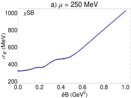
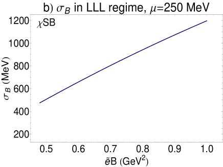
Figure 1: a) The dependence of $\sigma_{B}$ on $\tilde{e}B$ in the $\chi$SB phase for $\mu=250$ MeV; b) The analytical result of $\sigma_{B}$ in the regime of LLL dominance from (IV.9) is plotted for $\tilde{e}B\in\{0.45,1\}~{}\mbox{GeV}^{2}$ and $\mu=250$ MeV.

In Fig. 1a, the $\chi$SB mass gap $\sigma$ is plotted as a function of $\tilde{e}B$ and for fixed chemical potential $\mu=250$ MeV. Small oscillations for small value of $\tilde{e}B$ arise from the well-known van Alfven–de Haas (vAdH) effect alfven . They occur when the Landau levels pass the quark Fermi surface. They are also observed in inagaki2003 for the $\chi$SB mass gaps. Note that the oscillations are sharper, the smaller the value of the free parameter $A$ in (V.3) is chosen [see also ruggieri2009 for a discussion on the effect of free parameters in smooth cutoff functions (form factors)]. As for $\tilde{e}B\gtrsim 0.45$ GeV², where the dependence of $\sigma_{B}$ on $\tilde{e}B$ is almost linear, we enter in the regime of LLL dominance. The qualitative behavior of $\sigma_{B}$ as a function of $\tilde{e}B$ for strong magnetic fields can be checked by comparing our numerical result from Fig. 1a with the analytical result for $\sigma_{B}$ from (IV.9). The latter is plotted in Fig. 1b for the same interval of the magnetic field, i.e. $\tilde{e}B\in\{0.45,1\}~{}\mbox{GeV}^{2}$. Similarly, in Fig. 2a, the CSC mass gap $\Delta_{B}$ is plotted as a function of $\tilde{e}B$ for $\mu=460$ MeV. Same small vAdH oscillations appear for small $\tilde{e}B\lesssim 0.47$ GeV². They are also observed in warringa2007 and shovkovy2007 for the diquark in the CFL superconducting phase. Small oscillations in Fig. 2a, end up in a linear regime, that starts, as in the previous case, at $\tilde{e}B\gtrsim 0.47$ GeV². The qualitative behavior of $\Delta_{B}$ in this regime can be compared with the analytical result (IV.40), that arises in the LLL approximation (Fig. 2b).

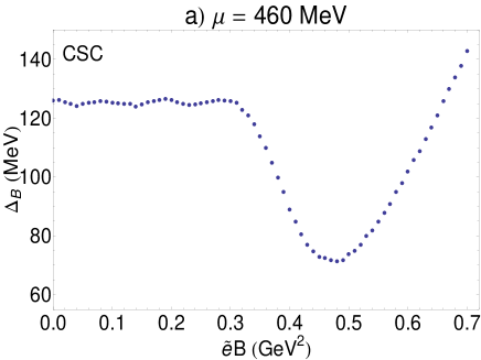
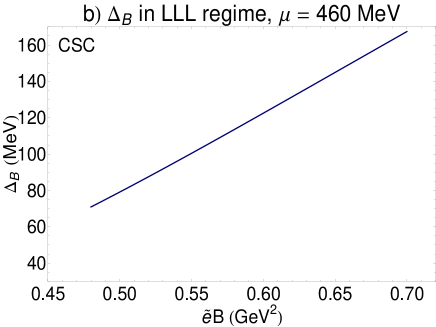
Figure 2: a) The dependence of $\Delta_{B}$ on $\tilde{e}B$ in the CSC phase for $\mu=460$ MeV. b) The analytical result of $\Delta_{B}$ in the regime of LLL dominance from (IV.40) is plotted for $\tilde{e}B\in\{0.47,1\}~{}\mbox{GeV}^{2}$.

In Fig. 3, the dependence of the color chemical potential $\mu_{8}$ on $\tilde{e}B$ is plotted for $\mu=460$ MeV in the CSC phase. The vAdH oscillations in Fig. 3 are similar to the oscillations of $\mu_{8}$ in the regime of small magnetic fields that are observed in warringa2007 in the superconducting CFL model.

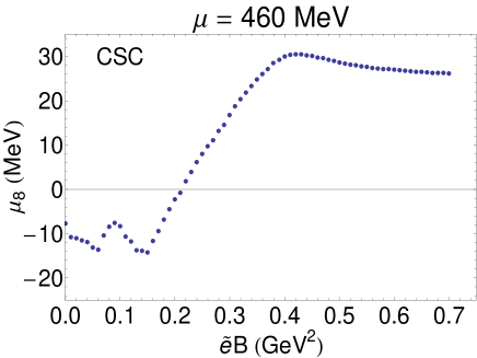
Figure 3: The dependence of $\mu_{8}$ on $\tilde{e}B$ in the CSC phase for $\mu=460$ MeV. The vAdH oscillations are similar to the oscillations that are observed in warringa2007 in the superconducting CFL model.

In summary, comparing the above numerical results with our analytical results from Sec. IV.A and IV.B for non-zero magnetic field, it turns out that there exists a threshold magnetic field $(\tilde{e}B)_{t}\simeq 0.45-0.50$ GeV², where the qualitative behavior of our numerical results coincides with the qualitative behavior of the analytical results for $\chi$SB and CSC mass gaps $\sigma_{B}$ and $\Delta_{B}$. This regime, for which the LLL approximation seems to be reliable, will be denoted from now on by “the linear regime”.

Using the above data, the magnetization of the 2SC superconducting medium can be studied as a function of $\tilde{e}B$ and for fixed chemical potential $\mu$. Fig. 4 shows the dependence of the product of the magnetization ${\mathbf{M}}=M{\mathbf{e}}_{3}$ with $M\equiv-\frac{\partial\Omega_{\mbox{\tiny{eff}}}^{(1)}}{\partial B}$ and the rotated magnetic field $\tilde{\mathbf{B}}=B{\mathbf{e}}_{3}$ as a function of $\tilde{e}B$ for two different chemical potential $\mu=250$ MeV in the $\chi$SB regime and $\mu=460$ MeV in the CSC regime (Figs. 4a and 4b). Here $\Omega_{\mbox{\tiny{eff}}}^{(1)}$ is the one-loop part of the effective potential (III.34). For simplicity, we will use the definition ${\mathbf{M}}\cdot\tilde{\mathbf{B}}\equiv-\tilde{e}B\frac{\partial\Omega_{\mbox{\tiny{eff}}}^{(1)}}{\partial\tilde{e}B}$. Equivalently, one can define the magnetization by introducing the Gibbs free energy density ${\cal{G}}$ in the presence of a constant magnetic field $B$

$${\cal{G}}(\sigma,\Delta;B,\mu)=\frac{B^{2}}{2}+\Omega_{\mbox{\tiny{eff}}}^{(1)}(\sigma,\Delta;B,\mu)-HB,$$ (V.3)

where $H$ is the external magnetic field shovkovy2007 . Whereas in vacuum $H=B$, in a medium with finite magnetization density, the external magnetic field $H$ is different from the induced magnetic field $B$. Minimizing ${\cal{G}}$ with respect to $B$ and evaluating the result at the minimum of the potential, we get the well-known relation ${\mathbf{M}}={\mathbf{B}}-{\mathbf{H}}$, where ${\mathbf{M}}$ is the magnetization. Note that the minimum of the potential in the $\chi$SB phase is given by $(\sigma_{B}\neq 0,\Delta_{B}=\mu_{8}=0)$ and in the CSC phase by $(\sigma_{B}=0,\Delta_{B}\neq 0,\mu_{8}\neq 0)$. The magnetization of the superconducting CFL phase is studied as a function of $eB/\mu^{2}$ for $\mu=500$ MeV in shovkovy2007 , where the same vAdH oscillations as appears in Fig. 4 are observed.

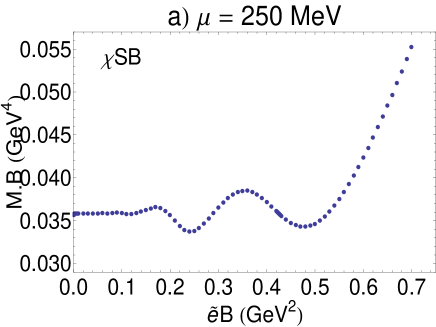
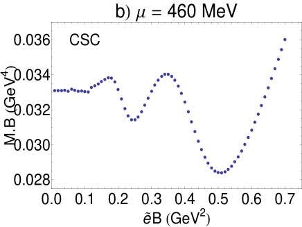
Figure 4: The dependence of the product ${\mathbf{M}}\cdot\tilde{\mathbf{B}}$ on the magnetic field of fixed chemical potential a) $\mu=250$ MeV in the $\chi$SB phase and b) $\mu=460$ MeV in the CSC phase. The linear regime in both phases starts at ${\tilde{e}}B\simeq 0.45-0.50$ GeV².

In what follows, we will first study the $\mu$-dependence of $\sigma_{B}$ and $\Delta_{B}$. We then present the phase diagram $\mu_{c}-\tilde{e}B$ of the 2SC quark matter at zero temperature. Let us start with the case of zero magnetic field. In Fig. 5, the $\mu$-dependence of $\sigma_{0}$ in the $\chi$SB phase, as well as $\Delta_{0}$ and $\mu_{8}$ in the CSC phase are plotted for zero magnetic field. For our specific choice of free parameters $\Lambda,G_{S}$ and $G_{D}$, $\sigma_{0}=323.8$ MeV for $\mu\leq\mu_{c}$. Here, the critical chemical potential $\mu_{c}=325$ MeV and the value of $\Delta_{0}$ for $\mu\simeq\mu_{c}$ is $\Delta_{0}=78.0$ MeV. Our results coincides qualitatively with the numerical results presented in ebert2005 (see also ebert2010 for a recent investigation of Cooper-pairing in NJL-type models).

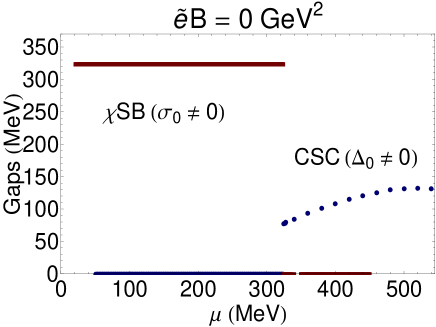
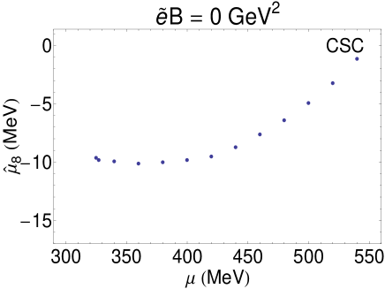
Figure 5: The $\mu$-dependence of $\sigma_{0}$ in the $\chi$SB phase, and $\Delta_{0}$ in the CSC phase for $\tilde{e}B=0$ (left panel). The $\mu$-dependence of $\mu_{8}$ for $\tilde{e}B=0$ (right panel).

We can compare the $\mu$-dependence of $\Delta_{0}^{2}$ arising from our numerical calculation with the relation (IV.46) arising from our analytical results for vanishing magnetic field. To do this we have fitted our numerical data with a function

$$\Delta_{0}^{2}(\mu)=(a-b\mu^{2})\exp\left(-\frac{c}{\mu^{2}}\right),$$ (V.4)

similar to (IV.46). Here, $a,b$ and $c$ are free parameters. The numerical values of these parameters arising from our fit are in good agreement with the expected analytical values arising from (IV.46) (see Fig. 6 and Table II). This can be quantified by defining

$$\eta\equiv\bigg{|}\frac{\mbox{Analytical value $-$ Numerical value}}{\mbox{(Analytical value $+$ Numerical value)/2}}\bigg{|},$$ (V.5)

as a measure for the variation of the numerical value with respect to the average of analytical and numerical values. In Table II, $\eta_{a},\eta_{b}$ and $\eta_{c}$ are less than $50$%. Note that the difference between the analytical and numerical values of $a,b$ and $c$ lies on the approximations that are made to determine analytically $\Delta_{0}^{2}$ in (IV.46).

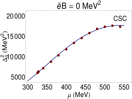
Figure 6: The dots are the numerical values of $\Delta_{0}^{2}$. The solid line is the corresponding fit of $\Delta_{0}^{2}(\mu)$ from (V.4). The fit parameters $a,b$ and $c$ are listed in Table II. The regression parameter $R^{2}$, as a measure of reliability of the numerical fit, is in this case $R^{2}=0.999852$.

	Analytical parameters			Numerical fit parameters			$\eta$ in %
$\tilde{e}B$ (GeV2)	$a$ (MeV2)	$b$	$c$ (MeV2)	$a$ (MeV2)	$b$	$c$ (MeV2)	$\eta_{a}$	$\eta_{b}$	$\eta_{c}$
$0$	$8.49\times 10^{4}$	$0.19$	$2.29\times 10^{5}$	$7.84\times 10^{4}$	$0.13$	$2.52\times 10^{5}$	$8$	$38$	$10$

Table 2: Numerical fit data for $\Delta_{0}^{2}(\mu)$ from (V.4). The numerical values of the parameters arising from our fit are in good agreement with the expected analytical values arising from (IV.46) [see $\eta_{a},\eta_{b}$ and $\eta_{c}$ with $\eta$ defined in (V.5)].

Let us now concentrate on the case of non-vanishing magnetic field. In Table III, we have summarized our numerical results for critical chemical potential $\mu_{c}$, the mass gap $\sigma_{B}$ for $\mu\leq\mu_{c}$ and the 2SC gap $\Delta_{B}$ at $\mu\simeq\mu_{c}$. The critical chemical potential $\mu_{c}$ and the $\chi$SB mass gaps $\sigma_{B}(\mu\leq\mu_{c})$ increase by increasing the external magnetic field. In the vicinity of the phase transition from $\chi$SB to CSC phase, the CSC mass gap $\Delta_{B}(\mu\simeq\mu_{c})$ also increases by increasing the magnetic field.

$\tilde{e}B$ in GeV2	$\mu_{c}$ in MeV	$\sigma_{B}(\mu\leq\mu_{c})$ in MeV	$\Delta_{B}(\mu\simeq\mu_{c})$ in MeV
$0.002$	$316.0$	$312.0$	$70.0$
$0.005$	$287.0$	$311.0$	$61.0$
$0.01$	$324.2$	$322.4$	$78.0$
$0.04$	$322.3$	$326.4$	$77.6$
$0.05$	$321.9$	$327.8$	$77.9$
$0.10$	$311.3$	$338.4$	$76.9$
$0.20$	$296.0$	$366.0$	$50.8$
$0.30$	$315.0$	$420.7$	$73.2$
$0.40$	$329.0$	$464.8$	$80.4$
$0.46$	$329.6$	$477.0$	$82.6$
$0.48$	$334.0$	$487.0$	$85.7$
$0.50$	$340.8$	$499.0$	$88.8$
$0.60$	$392.4$	$593.0$	$116.9$
$0.70$	$450.7$	$700.0$	$147.7$

Table 3: Numerical results for critical chemical potential $\mu_{c}$, the mass gap $\sigma_{B}$ for $\mu\leq\mu_{c}$ and the 2SC gap $\Delta_{B}$ at $\mu\simeq\mu_{c}$.

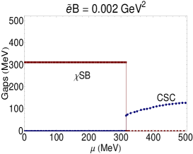
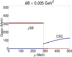
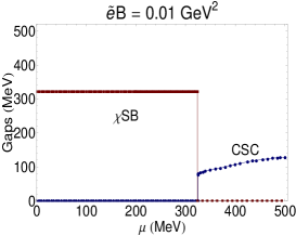
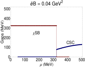
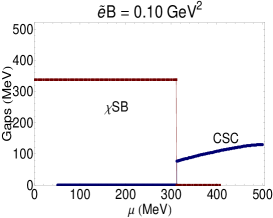
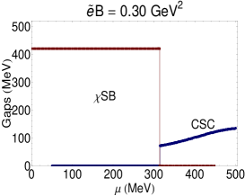
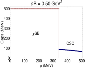
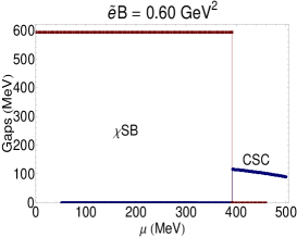
Figure 7: The $\mu$-dependence of $\sigma_{B}$ in the $\chi$SB phase (red lines), and $\Delta_{B}$ in the CSC phase (blue lines) for different values of $\tilde{e}B$. The $\chi$SB mass gap $\sigma_{B}(\mu,\tilde{e}B)$ is constant in $\mu\leq\mu_{c}$ and increases for increasing $\tilde{e}B$. The critical chemical potential $\mu_{c}$ increases for increasing $\tilde{e}B$. For our specific choice of parameters ($m_{0}=0,G_{D}<G_{S}$) no mixed phase appears. The CSC mass gap $\Delta_{B}$ exists therefore only at $\mu>\mu_{c}$. The slopes of the curves appearing at $\mu>\mu_{c}$ are decreasing for increasing $\tilde{e}B$. The first order nature of the phase transition between $\chi$SB and CSC phases is visible. The dependence of the $\chi$SB and CSC gaps for vanishing magnetic field is also considered here to have a comparison with the $\mu$-dependence of the gaps for non-vanishing $\tilde{e}B$.

The $\mu$-dependence of $\sigma_{B}$ and $\Delta_{B}$ are presented also in Fig. 7. There is a first order phase transition from the $\chi$SB to the CSC phase [see also Fig. 9 for more detail on the phase structure in $\mu_{c}-\tilde{e}B$ plane]. Because of our specific choice $m_{0}=0$ and $G_{D}<G_{S}$, no mixed broken phase appears at $\mu>\mu_{c}$ huang2002 , and the $\chi$SB mass gap $\sigma_{B}(\mu)$ is constant for $\mu\leq\mu_{c}$. For small value of $\tilde{e}B$, the CSC mass gap $\Delta_{B}(\mu,\tilde{e}B)$, is increasing with $\mu$. The magnetic field enhances the chiral symmetry breaking. This is known as the phenomenon of magnetic catalysis miransky1995 , which is also observed in inagaki2003 . In the linear regime, i.e. for $\tilde{e}B\gtrsim 0.45$ GeV², $\Delta_{B}$ is decreasing with $\mu$. To study the linear regime in detail, we have fitted our numerical data for $\Delta_{B}$ as a function of $\mu$ and fixed $\tilde{e}B$, with a function similar to (IV.40)

$$\Delta_{B}^{2}=(a-b\mu^{2}),$$ (V.6)

where $a$ and $b$ are free parameters, that depend on $\tilde{e}B$. In Table IV, we have compared the expected analytical results for the parameters $a$ and $b$, with the corresponding results from fitting our numerical data with (V.6) for different $\tilde{e}B$. For $\tilde{e}B\gtrsim 0.44$ GeV², $\eta_{a}$ and $\eta_{b}$ are less than $50$%.

	Analytical parameters		Numerical fit parameters		$\eta$ in %
$\tilde{e}B$ (GeV${}^{2})$	$a$ (MeV2)	$b$	$a$ (MeV2)	$b$	$\eta_{a}$	$\eta_{b}$
$0.04$	$5.27\times 10^{-24}$	$1.32\times 10^{-28}$	$-1.06\times 10^{3}$	$-0.077$	$200$	$200$
$0.10$	$1.62\times 10^{-6}$	$1.62\times 10^{-11}$	$-8.37\times 10^{2}$	$-0.077$	$200$	$200$
$0.30$	$1.91\times 10^{2}$	$6.37\times 10^{-4}$	$-4.53\times 10^{3}$	$-0.094$	$218$	$201$
$0.40$	$2.27\times 10^{3}$	$0.006$	$+4.17\times 10^{3}$	$-0.018$	$59$	$400$
$0.44$	$4.53\times 10^{3}$	$0.010$	$+7.38\times 10^{3}$	$+0.008$	$48$	$22$
$0.46$	$6.14\times 10^{3}$	$0.013$	$+8.47\times 10^{3}$	$+0.015$	$32$	$14$
$0.50$	$1.05\times 10^{4}$	$0.021$	$+1.09\times 10^{4}$	$+0.025$	$4$	$17$
$0.60$	$3.03\times 10^{4}$	$0.050$	$+2.26\times 10^{4}$	$+0.058$	$29$	$15$

Table 4: Numerical fit data for $\Delta_{B}^{2}$ as a function of $\mu$ from (V.6). In the linear regime, i.e. for $\tilde{e}B\gtrsim 0.45$ GeV², the numerical values of the parameters arising from our fit are in good agreement with the expected analytical values of the parameters from (IV.40) [see $\eta_{a}$ and $\eta_{b}$ with $\eta$ defined in (V.5)].

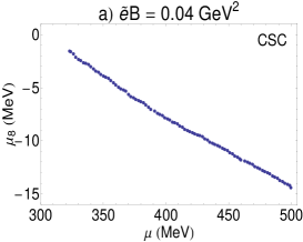
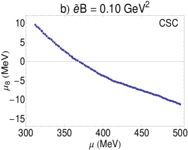
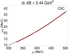
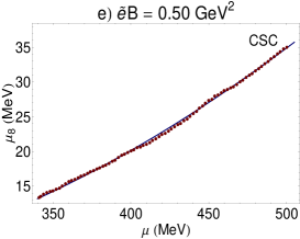
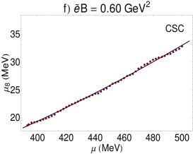
Figure 8: The $\mu$-dependence of the color chemical potential $\mu_{8}$ as a function. The numerical data for $\mu_{8}$ are fitted in Figs $8d-8f$ by (V.7). In the linear regime, the fitted curves [solid (blue) lines in $8d-8f$] are in good agreement with our numerical data. For $\tilde{e}B=0.44,0.5$ GeV² and $0.6$ GeV², the regression parameter $R^{2}$, as a measure of reliability of numerical fits are $R^{2}=0.999991,0.999924,0.999952$, respectively.

In Fig. 8, the $\mu$-dependence of the color chemical potential $\mu_{8}$ for different $\tilde{e}B$ is demonstrated. As in the previous cases, we expect that, in the linear regime $\tilde{e}B\gtrsim 0.45$ GeV², the $\mu$ dependence of $\mu_{8}$ is given by a function similar to (IV.37), that arises analytically in the LLL approximation. We define therefore a function

$$\mu_{8}=\frac{\mu^{3}}{a+b\mu^{2}},$$ (V.7)

with arbitrary, $\tilde{e}B$-dependent parameters $a$ and $b$. In Table V, we have compared the data that arise numerically by fitting the numerical values of $\mu_{8}$ with (V.7) for different $\tilde{e}B$. As in the previous case, the difference between the numerical fit data and the expected analytical values of $a$ and $b$ arising from (IV.37) minimizes in the linear regime for $\tilde{e}B\gtrsim 0.40$ GeV² ($\eta_{a}$ and $\eta_{b}$ in Table V are less than $50$%.).

	Analytical parameters		Numerical fit parameters		$\eta$ in %
$\tilde{e}B$ (GeV2)	$a$ (MeV2)	$b$	$a$ (MeV2)	$b$	$\eta_{a}$	$\eta_{b}$
$0.04$	$1.80\times 10^{5}$	$6$	$-1.01\times 10^{7}$	$+7.53$	$207$	$23$
$0.10$	$4.50\times 10^{5}$	$6$	$-4.93\times 10^{7}$	$+161.14$	$204$	$186$
$0.30$	$1.35\times 10^{6}$	$6$	$+3.04\times 10^{6}$	$+13.04$	$77$	$74$
$0.40$	$1.80\times 10^{6}$	$6$	$+1.93\times 10^{6}$	$+6.27$	$7$	$4$
$0.44$	$1.98\times 10^{6}$	$6$	$+2.34\times 10^{6}$	$+4.11$	$17$	$37$
$0.46$	$2.07\times 10^{6}$	$6$	$+2.43\times 10^{6}$	$+3.89$	$16$	$43$
$0.50$	$2.25\times 10^{6}$	$6$	$+2.46\times 10^{6}$	$+4.49$	$9$	$29$
$0.60$	$2.70\times 10^{6}$	$6$	$+2.45\times 10^{6}$	$+5.35$	$10$	$11$

Table 5: Numerical fit data for $\mu_{8}$ as a function of $\mu$ from (V.7). In the linear regime, i.e. for $\tilde{e}B\gtrsim 0.40$ GeV², the numerical values of the parameters arising from our fit are in good agreement with the expected analytical values of the parameters from (IV.37) [see $\eta_{a}$ and $\eta_{b}$ with $\eta$ defined in (V.5)].

Finally, we will present the phase structure of the model in a $\mu_{c}-\tilde{e}B$ plane in Fig. 9. In particular, we are interested on the effect of the color chemical potential $\mu_{8}$ on the phase structure of the model. In Fig. 9a (Fig. 9b) the phase structure for $\mu_{8}=0$ ($\mu_{8}\neq 0$) is plotted. Because of our specific choice of parameters, we expect $\chi$SB and CSC phase without mixing. A normal phase can also exist, where the mass gaps $\sigma_{B}$ and $\Delta_{B}$ corresponding to $\chi$SB and CSC phases vanish identically. To check this, we consider the gap equations and the color neutrality condition (IV). We have looked for the global minima of the system in two different regimes: $\mu_{c}\simeq 350-450$ MeV and $\mu_{c}\simeq 750-800$ MeV. As it turns out, in the first regime corresponding to $\mu_{c}\simeq 350-450$ MeV, the minima of $\Omega_{\mbox{\tiny{eff}}}$ from (III.34) are given by $(\sigma_{B}\neq 0,\Delta_{B}=0,\mu_{8}=0)$ for $\mu<\mu_{c}$ as well as $(\sigma_{B}=0,\Delta_{B}\neq 0,\mu_{8}\neq 0)$ for $\mu>\mu_{c}$. In the second regime corresponding to $\mu_{c}\simeq 750-800$ MeV, however, the global minima are $(\sigma_{B}=0,\Delta_{B}\neq 0,\mu_{8}\neq 0)$ for $\mu<\mu_{c}$, as well as $(\sigma_{B}=0,\Delta_{B}=0,\mu_{8}=0)$ for $\mu>\mu_{c}$. We conclude therefore that a phase transition from $\chi$SB to CSC phase occurs in the first regime at $\mu_{c}\simeq 350-450$ MeV, and a phase transition from CSC to the normal phase occurs in the second regime $\mu_{c}\simeq 750-800$ MeV. In the following, we denote the value of $\Omega_{\mbox{\tiny{eff}}}$ at the global minima by $\Omega_{\mbox{\tiny{$\chi$SB}}}\equiv\Omega_{\mbox{\tiny{eff}}}(\sigma_{B},0,0;\mu,\tilde{e}B)$, $\Omega_{\mbox{\tiny{CSC}}}\equiv\Omega_{\mbox{\tiny{eff}}}(0,\Delta_{B},\mu_{8};\mu,\tilde{e}B)$, and $\Omega_{\mbox{\tiny{Normal}}}\equiv\Omega_{\mbox{\tiny{eff}}}(0,0,0;\mu,\tilde{e}B)$ corresponding to the $\chi$SB, CSC and the normal phase, respectively. For different values of $(\mu,\tilde{e}B)$, the $\chi$SB phase is defined by $\Omega_{\mbox{\tiny{$\chi$SB}}}\leq\Omega_{\mbox{\tiny{CSC}}}$ and the CSC phase by $\Omega_{\mbox{\tiny{CSC}}}\leq\Omega_{\mbox{\tiny{$\chi$SB}}}$. Moreover, the exact value of $\mu_{c}$ for the first order phase transition from $\chi$SB to the CSC phase [the lower (red) solid line in Fig. 9a and 9b] and from the CSC phase to the $\chi$SB phase [(green) solid line in Fig. 9b] are then defined by $\Omega_{\mbox{\tiny{$\chi$SB}}}=\Omega_{\mbox{\tiny{CSC}}}$ and $\Omega_{\mbox{\tiny{CSC}}}=\Omega_{\mbox{\tiny{Normal}}}$, respectively sato1998 . As for the second order phase transition between the CSC and the normal phase, an analysis similar to berges1998 is performed.

Figure 9: The phase diagram of 2SC model is plotted in a $\mu_{c}-\tilde{e}B$ plane for a) $\mu_{8}=0$ and b) $\mu_{8}\neq 0$. The solid (red) lines in a) and b) indicate first order phase transitions between the $\chi$SB and the CSC phase. The dashed (black) lines in a) and b) are second order critical lines between the CSC and the normal phase. As it is shown in b), for $\mu_{8}\neq 0$ and at $\mu_{c}\simeq 755$ MeV and $\tilde{e}B\simeq 0.13$ GeV², the second order phase transition goes over into a first order phase transition between the CSC and the normal phase [solid (green) line]. At $\tilde{e}B\simeq 0.4$ GeV², $\mu_{c}$ suddenly decreases and increases once again by increasing the external magnetic fields in the CSC regime.

In Fig. 9a, the phase diagram of the 2SC model in a $\mu_{c}-\tilde{e}B$ plane is plotted for vanishing $\mu_{8}$. A first order phase transition occurs between the $\chi$SB and the CSC phase in the regime $\mu_{c}\simeq 350-450$ MeV (solid red line). This confirms the results by mandal2009 , where a first order phase transition is observed for fixed value of $\tilde{e}B=0.05$ GeV², and various $G_{D}/G_{S}$. The transition from the CSC into the normal phase is of second order and occurs in the regime $\mu_{c}\simeq 750-800$ MeV (dashed black line). According to the phase diagram for nonvanishing $\mu_{8}$ in Fig. 9b, however, whereas the transition from the $\chi$SB to CSC phase is still of first order (solid red line), the second order phase transition for small values of $\tilde{e}B$ (dashed black line) goes over into a first order phase transition at $\mu_{c}\simeq 755$ MeV and $\tilde{e}B\simeq 0.13$ GeV² (solid green line). Moreover, at $\tilde{e}B\simeq 0.4$ GeV², $\mu_{c}$ suddenly decreases and increases once again by increasing the external magnetic fields in the CSC regime. The CSC regime is nevertheless suppressed in the linear regime $\tilde{e}B\gtrsim 0.45$ GeV² by the external magnetic field (see Fig. 9b).

VI Concluding remarks

In this paper, we have studied the effect of constant magnetic fields on the formation of bound states in the chiral as well as the color symmetry breaking phase. In the first part of the paper, after introducing a two-flavor NJL type model including meson and diquark condensates, we have computed the one-loop effective action and the thermodynamic potential of the theory at zero temperature and finite density. Neglecting the quark mass $m_{0}$ and choosing the diquark-to-chiral coupling ratio $G_{D}/G_{S}<1$ huang2002 , we can consider the $\chi$SB and CSC phases separately. The $\chi$SB and CSC mass gaps $\sigma_{B}$ and $\Delta_{B}$ as well as the color chemical potential $\mu_{8}$ are determined analytically in the limit of very strong magnetic fields. In this limit, the dynamics of the system is dominated by the lowest Landau level and therefore the effect of all higher Landau levels are negligible. According to miransky1995 , in this limit, as a result of dimensional reduction from $D$ to $D-2$ dimensions, the formation of bound states and consequently a dynamical symmetry breaking will be possible even for weak interactions between two fermions. This is the phenomenon of magnetic catalysis, discussed widely in the literature in the past few years cosmology ; condensed ; particle . Denoting the dimensionless coupling constants in the $\chi$SB and CSC phases by $g_{s}\sim G_{S}\Lambda^{2}$ and $g_{d}\sim G_{D}\Lambda^{2}$, we have determined the mass gaps for different regimes of $g_{s}$ and $g_{d}$. Here, $\Lambda$ is certain momentum cutoff. In ebert2005 , the $\chi$SB and CSC mass gaps of a similar 2SC model was determined numerically for vanishing magnetic field. Introducing a large momentum cutoff $\Lambda$ and performing appropriate approximations, we have determined analytically the mass gaps $\sigma_{0}$ and $\Delta_{0}$ as well as $\mu_{8}$ corresponding to $\chi$SB and CSC phases for zero magnetic field too.

In the second part of the paper, a detailed numerical analysis is performed to explore the effect of any arbitrary magnetic field on the mass gaps $\sigma$ and $\Delta$ and the color chemical potential $\mu_{8}$. First, the dependence of $\sigma$ and $\Delta$ on various $\tilde{e}B\in[0,1]$ GeV² is plotted for fixed $\mu=250$ MeV and $\mu=460$ MeV in the $\chi$SB and CSC phases, respectively. For small values of $\tilde{e}B$, we observe small van Alfven-de Haas oscillations, that appear, according to warringa2007 ; shovkovy2007 also in the CFL phase for $\mu=500$ MeV. Same oscillations appears also in the magnetization $M$ for the same fixed value of chemical potentials. At $\tilde{e}B\simeq 0.4-0.5$ GeV², the oscillations end up in a linear regime, where we believe that the dynamics of the system is described exclusively by the LLL. This can be checked by comparing qualitatively the numerical dependence of $\sigma_{B}$ and $\Delta_{B}$ for $\tilde{e}B\geq 0.45$ GeV² and fixed $\mu$. The $\mu$-dependence of $\sigma$ and $\Delta$ are then considered for various $\tilde{e}B$. Our numerical results for vanishing magnetic field coincide with the numerical results presented in ebert2005 . The $\mu$-dependence of $\sigma_{B}$ and $\Delta_{B}$ as well as $\mu_{8}$ are then considered for various finite $\tilde{e}B$. The numerical results in the linear regime, i.e. for $\tilde{e}B\gtrsim 0.45$ GeV² are comparable with our before mentioned analytical results in the limit of large $\tilde{e}B$. This is shown using appropriate numerical fits. The phase structure of the $\chi$SB and CSC phases in a $\mu_{c}-\tilde{e}B$ plane is also presented. We are in particular interested on the effect of the color chemical potential $\mu_{8}$ on the phase diagram of the model. For both $\mu_{8}=0$ as well as $\mu_{8}\neq 0$, the transition from the $\chi$SB phase into the CSC phase is of first order, and occurs in the regime $\mu_{c}\simeq 350-450$ MeV and for $\tilde{e}B\in[0,0.7]$ GeV² (see Fig. 9a). This confirms the result in mandal2009 , where a first order phase transition is observed between the $\chi$SB and CSC phase for fixed $\tilde{e}B=0.05$ GeV² and various $G_{D}/G_{S}$ ratios. Assuming that the CSC phase goes over into a normal phase at $\mu>500$ MeV, it turns out that whereas for $\mu_{8}=0$, this transition is of second order, for nonvanishing $\mu_{8}$, a second order phase transition occurs first for small $\tilde{e}B$. It goes then over into a first order phase transition at $\mu_{c}\simeq 755$ MeV and $\tilde{e}B\simeq 0.13$ GeV². At $\tilde{e}B\simeq 0.4$ GeV², $\mu_{c}$ suddenly decreases and increases once again by increasing the external magnetic fields. The CSC phase is nevertheless suppressed in the linear regime $\tilde{e}B\gtrsim 0.45$ GeV² by the external magnetic field (see Fig. 9b).

At the end, let us just emphasize that the study of color superconductivity in the presence of constant magnetic fields has not only astrophysical consequences in forming the structure of compact star cores, it may be also relevant for future heavy ion collision experiments. Recently in blaschke2010 , the accessibility of the color superconducting 2SC phase in the heavy ion collisions is investigated. It is stated that for high enough collision energies the 2SC may be accessible in future collision experiments. On the other hand, there are various evidences of the creation of very strong magnetic fields in non-central heavy ion collisions skokov ; kharzeev51-STAR . It would be interesting to perform similar analysis as in blaschke2010 considering the presence of constant magnetic fields. To do this, the effect of finite temperature on the phase diagram of the 2SC superconducting phase in the presence of constant magnetic fields has also to be considered. This will be reported in future publications sadooghi2010 .

VII Acknowledgments

Sh. F. thanks F. Farahpour for useful discussions on numerical results, and H. Hadipour for discussions on high $T_{c}$-superconductivity, N. S. thanks M. Bahmanabadi and S. Rahvar for discussions on the numerical fit data. Both authors thank F. Ardalan, H. Arfaei, A. E. Mosaffa for discussions and E. J. Ferrer for email correspondence.

References

(1)
D. Bailin and A. Love,
Superconductivity in quark matter, Nucl. Phys. B 205, 119 (1982).
M. G. Alford, K. Rajagopal and F. Wilczek,
Color-flavor locking and chiral symmetry breaking in high density QCD,
Nucl. Phys. B 537, 443 (1999), arXiv: hep-ph/9804403.
D. T. Son,
Superconductivity by long-range color magnetic interaction in high-density
quark matter,
Phys. Rev. D 59, 094019 (1999), arXiv: hep-ph/9812287.
T. Schafer and F. Wilczek,
Superconductivity from perturbative one-gluon exchange in high density
quark matter,
Phys. Rev. D 60, 114033 (1999), arXiv: hep-ph/9906512.
D. K. Hong, V. A. Miransky, I. A. Shovkovy and L. C. R. Wijewardhana,
Schwinger-Dyson approach to color superconductivity in dense QCD,
Phys. Rev. D 61, 056001 (2000), [Erratum-ibid. D 62, 059903
(2000)], arXiv: hep-ph/9906478.
R. D. Pisarski and D. H. Rischke,
Gaps and critical temperature for color
superconductivity, Phys. Rev. D 61, 051501 (2000), arXiv: nucl-th/9907041.
(2)
Y. Nambu and G. Jona-Lasinio,
Dynamical model of elementary particles based on an analogy with
superconductivity. I,
Phys. Rev. 122, 345 (1961).
Y. Nambu and G. Jona-Lasinio,
Dynamical model of elementary particles based on an analogy with
superconductivity. II,
Phys. Rev. 124, 246 (1961).
(3)
M. G. Alford, K. Rajagopal and F. Wilczek,
QCD at finite baryon density: Nucleon droplets and color
superconductivity, Phys. Lett. B 422, 247 (1998), arXiv: hep-ph/9711395.
R. Rapp, T. Schafer, E. V. Shuryak and M. Velkovsky,
Diquark Bose condensates in high density matter and instantons,
Phys. Rev. Lett. 81, 53 (1998), arXiv: hep-ph/9711396.
(4)
M. G. Alford,
Color superconducting quark matter,
Ann. Rev. Nucl. Part. Sci. 51, 131 (2001), arXiv: hep-ph/0102047.
K. Rajagopal and F. Wilczek,
The condensed matter physics of QCD, arXiv:hep-ph/0011333.
G. Nardulli,
Effective description of QCD at very high densities,
Riv. Nuovo Cim. 25N3, 1 (2002), arXiv: hep-ph/0202037.
(5)
M. Buballa,
NJL model analysis of quark matter at large density,
Phys. Rept. 407, 205 (2005), arXiv: hep-ph/0402234.
M. Huang,
Color superconductivity at moderate baryon density,
Int. J. Mod. Phys. E 14, 675
(2005), arXiv: hep-ph/0409167.
I. A. Shovkovy,
Two lectures on color superconductivity,
Found. Phys. 35, 1309 (2005), arXiv: nucl-th/0410091.
M. G. Alford, A. Schmitt, K. Rajagopal and T. Schafer,
Color superconductivity in dense quark matter,
Rev. Mod. Phys. 80, 1455 (2008), arXiv: 0709.4635 [hep-ph].
(6)
D. Ebert, K. G. Klimenko and V. L. Yudichev,
Mesons and diquarks in the color neutral 2SC phase of dense cold quark
matter, Phys. Rev. D 72, 056007 (2005), arXiv: hep-ph/0504218.
(7)
J. Berges and K. Rajagopal,
Color superconductivity and chiral symmetry restoration at nonzero baryon
density and temperature,
Nucl. Phys. B 538, 215 (1999), arXiv: hep-ph/9804233.
(8)
T. M. Schwarz, S. P. Klevansky and G. Papp,
The phase diagram and bulk thermodynamical quantities in the NJL model at
finite temperature and density,
Phys. Rev. C 60, 055205 (1999), arXiv: nucl-th/9903048.
B. Vanderheyden and A. D. Jackson,
Random matrix model for chiral symmetry breaking and color
superconductivity in QCD at finite density,
Phys. Rev. D 62, 094010 (2000), arXiv: hep-ph/0003150.
(9)
M. Huang, P. f. Zhuang and W. q. Chao,
Charge neutrality effects on 2-flavor color superconductivity,
Phys. Rev. D 67, 065015 (2003), arXiv: hep-ph/0207008.
(10)
M. Buballa and I. A. Shovkovy,
A note on color neutrality in NJL-type models,
Phys. Rev. D 72, 097501 (2005), [arXiv:hep-ph/0508197].
(11)
Sh. Fayyazbakhsh and N. Sadooghi, work in preparation.
(12)
C. Thompson and R. C. Duncan,
The soft gamma repeaters as very strongly magnetized neutron stars. 2.
Quiescent neutrino, x-ray, and Alfven wave emission, Astrophys. J. 473 (1996) 322.
(13)
V. de la Incera,
Nonperturbative Physics in a Magnetic Field, arXiv: 1004.4931 [hep-ph].
(14)
D. E. Kharzeev, L. D. McLerran and H. J. Warringa,
The effects of topological charge change in heavy ion collisions: ’Event by
event P and CP violation’,
Nucl. Phys. A 803, 227 (2008), arXiv: 0711.0950 [hep-ph].
H. J. Warringa,
Implications of CP-violating transitions in hot quark matter on heavy ion
collisions,
J. Phys. G 35, 104012 (2008), arXiv: 0805.1384 [hep-ph].
(15)
I. V. Selyuzhenkov [STAR Collaboration],
Global polarization and parity violation study in Au + Au collisions,
Rom. Rep. Phys. 58, 049 (2006), arXiv: nucl-ex/0510069.
(16)
V. Skokov, A. Y. Illarionov and V. Toneev,
Estimate of the magnetic field strength in heavy-ion collisions,
Int. J. Mod. Phys. A 24, 5925 (2009), arXiv: 0907.1396 [nucl-th].
(17)
D. B. Blaschke, F. Sandin, V. V. Skokov and S. Typel,
Accessibility of color superconducting quark matter phases in heavy-ion
collisions, arXiv: 1004.4375 [hep-ph].
(18)
M. G. Alford, J. Berges and K. Rajagopal,
Magnetic fields within color superconducting neutron star cores,
Nucl. Phys. B 571, 269 (2000), arXiv: hep-ph/9910254.
(19)
E. V. Gorbar,
On color superconductivity in external magnetic field, Phys. Rev. D 62, 014007
(2000), arXiv: hep-ph/0001211.
(20)
E. J. Ferrer, V. de la Incera and C. Manuel,
Color-superconducting gap in the presence of a magnetic field,
Nucl. Phys. B 747, 88 (2006), arXiv: hep-ph/0603233.
E. J. Ferrer and V. de la Incera,
Chromomagnetic Instability and Induced Magnetic Field in Neutral Two-Flavor
Color Superconductivity,
Phys. Rev. D 76, 114012 (2007), arXiv: 0705.2403 [hep-ph].
(21)
E. J. Ferrer, V. de la Incera and C. Manuel,
Magnetic color flavor locking phase in high density QCD,
Phys. Rev. Lett. 95, 152002 (2005), arXiv: hep-ph/0503162.
E. J. Ferrer and V. de la Incera,
Magnetic phases in three-flavor color superconductivity,
Phys. Rev. D 76, 045011 (2007), arXiv: nucl-th/0703034.
(22)
K. Fukushima and H. J. Warringa,
Color superconducting matter in a magnetic field,
Phys. Rev. Lett. 100, 032007 (2008), arXiv: 0707.3785 [hep-ph].
(23)
J. L. Noronha and I. A. Shovkovy,
Color-flavor locked superconductor in a magnetic field,
Phys. Rev. D 76, 105030 (2007), arXiv: 0708.0307 [hep-ph].
(24)
D. Ebert and A. S. Vshivtsev,
Van Alphen-de Haas effect for dense cold quark matter in a homogeneous
magnetic field, arXiv:hep-ph/9806421.
(25)
M. G. Alford and A. Sedrakian,
Color-magnetic flux tubes in quark matter cores of neutron stars, arXiv: 1001.3346 [astro-ph.SR].
X. G. Huang, M. Huang, D. H. Rischke and A. Sedrakian,
Anisotropic Hydrodynamics, Bulk Viscosities and R-Modes of Strange Quark
Stars with Strong Magnetic Fields,
Phys. Rev. D 81, 045015 (2010), arXiv: 0910.3633 [astro-ph.HE].
(26)
T. Mandal, P. Jaikumar and S. Digal,
Chiral and diquark condensates at large magnetic field in two-flavor
superconducting quark matter, arXiv: 0912.1413 [nucl-th].
(27)
V. I. Ritus, Ann. Phys. 69, 555 (1972); Sov. Phys. JETP 48, 788 (1978) [Zh. Eksp. Teor. Fiz. 75, 1560 (1978)].
(28)
E. Elizalde, E. J. Ferrer and V. de la Incera,
Neutrino self-energy and index of refraction in strong magnetic field: A
new approach, Annals Phys. 295, 33 (2002), arXiv: hep-ph/0007033.
(29)
K. Fukushima, D. E. Kharzeev and H. J. Warringa,
Electric-current susceptibility and the chiral magnetic
effect, arXiv: 0912.2961 [hep-ph].
(30)
K. G. Klimenko,
Three-dimensional Gross-Neveu model at nonzero temperature and in an
external magnetic field,
Z. Phys. C 54, 323 (1992).
V. P. Gusynin, V. A. Miransky and I. A. Shovkovy,
Catalysis of dynamical flavor symmetry breaking by a magnetic field in
(2+1)-dimensions,
Phys. Rev. Lett. 73, 3499 (1994)
[Erratum-ibid. 76, 1005 (1996)], arXiv: hep-ph/9405262.
(31)
V. P. Gusynin, V. A. Miransky and I. A. Shovkovy,
Dimensional reduction and catalysis of dynamical symmetry breaking by a
magnetic field,
Nucl. Phys. B 462, 249 (1996), arXiv: hep-ph/9509320.
D. S. Lee, C. N. Leung and Y. J. Ng,
Chiral symmetry breaking in a uniform external magnetic field,
Phys. Rev. D 55, 6504 (1997), arXiv: hep-th/9701172.
(32)
E. Elizalde, E. J. Ferrer and V. de la Incera,
Neutrino propagation in a strongly magnetized medium,
Phys. Rev. D 70, 043012 (2004).
E. J. Ferrer and V. de la Incera,
Neutrino propagation and oscillations in a strong magnetic field,
Int. J. Mod. Phys. A 19, 5385 (2004).
(33)
K. Farakos and N. E. Mavromatos,
Hidden non-Abelian gauge symmetries in doped planar antiferromagnets,
Phys. Rev. B 57, 3017 (1998).
V. C. Zhukovsky, K. G. Klimenko, V. V. Khudyakov and D. Ebert,
Magnetic catalysis of parity breaking in a massive Gross-Neveu model and
high-temperature superconductivity,
JETP Lett. 73, 121 (2001)
[Pisma Zh. Eksp. Teor. Fiz. 73, 137 (2001)], arXiv: hep-th/0012256.
E. J. Ferrer, V. P. Gusynin and V. de la Incera,
Magnetic field induced gap and kink behavior of thermal conductivity in
cuprates,
Mod. Phys. Lett. B 16, 107 (2002).
E. V. Gorbar, V. P. Gusynin, V. A. Miransky and I. A. Shovkovy,
Dynamics in the quantum Hall effect and the phase diagram of graphene,
Phys. Rev. B 78, 085437 (2008), arXiv: 0806.0846 [cond-mat.mes-hall].
(34)
K. G. Klimenko and V. C. Zhukovsky,
Does there arise a significant enhancement of the dynamical quark mass in a
strong magnetic field?,
Phys. Lett. B 665, 352 (2008), arXiv: 0803.2191 [hep-ph].
E. Rojas, A. Ayala, A. Bashir and A. Raya,
Dynamical mass generation in QED with magnetic fields: arbitrary field
strength and coupling constant, Phys. Rev. D 77, 093004
(2008), arXiv: 0803.4173 [hep-ph].
N. Sadooghi and K. S. Anaraki,
Improved ring potential of QED at finite temperature and in the presence of
weak and strong magnetic field, Phys. Rev. D 78, 125019 (2008), arXiv: 0805.0078 [hep-ph].
E. J. Ferrer and V. de la Incera,
Dynamically induced Zeeman effect in massless QED,
Phys. Rev. Lett. 102, 050402 (2009), arXiv:0807.4744 [hep-ph].
A. Ayala, A. Bashir, A. Raya and A. Sanchez,
Chiral phase transition in relativistic heavy-ion collisions with weak
magnetic fields: ring diagrams in the linear sigma model, Phys. Rev. D 80, 036005
(2009), arXiv: 0904.4533 [hep-ph].
E. J. Ferrer and V. de la Incera,
Dynamically generated anomalous magnetic moment in massless QED,
Nucl. Phys. B 824, 217 (2010), arXiv: 0905.1733 [hep-ph].
N. Sadooghi,
Chiral MHD description of a perfect magnetized QGP using the effective NJL
model in a strong magnetic field, arXiv: 0905.2097 [hep-ph].
A. Ayala, A. Bashir, A. Raya and A. Sanchez,
Impact of a uniform magnetic field and nonzero temperature on explicit
chiral symmetry breaking in QED: Arbitrary hierarchy of energy scales,
J. Phys. G 37, 015001 (2010), arXiv: 0910.1886 [hep-ph].
(35)
T. Inagaki, D. Kimura and T. Murata,
Four-fermion interaction model in a constant magnetic field at finite
temperature and chemical potential, Prog. Theor. Phys. 111, 371 (2004), arXiv: hep-ph/0312005.
(36)
D. P. Menezes, M. Benghi Pinto, S. S. Avancini, A. Perez Martinez and C. Providencia,
Quark matter under strong magnetic fields in the Nambu–Jona-Lasinio
Model,
Phys. Rev. C 79, 035807 (2009), arXiv: 0811.3361 [nucl-th].
(37)
S. B. Ruester,
The phase diagram of neutral quark matter, arXiv: nucl-th/0612090.
(38)
R. M. Coreless, G. H. Gonnet, D. E. G. Hare, D. J. Jeffrey and
D. E. Knuth, On the Lambert W function, Adv. Comput. Math.
5, 329 (1996).
(39)
D. Ebert and K. G. Klimenko,
Cooper pairing and finite-size effects in a NJL-type four-fermion model,
arXiv: 1005.0699 [hep-ph].
(40)
L. Campanelli and M. Ruggieri,
Probing the QCD vacuum with an abelian chromomagnetic field: A study within
an effective model, Phys. Rev. D 80, 034014 (2009), arXiv: 0905.0853 [hep-ph].
(41)
S. Kanemura, H. T. Sato and H. Tochimura,
Thermodynamic Gross-Neveu model under constant electromagnetic field,
Nucl. Phys. B 517, 567 (1998), arXiv: hep-ph/9707285.