Manufacturing time operators: covariance, selection criteria, and examples

Abstract

We provide the most general forms of covariant and normalized time operators and their probability densities, with applications to quantum clocks, the time of arrival, and Lyapunov quantum operators. Examples are discussed of the profusion of possible operators and their physical meaning. Criteria to define unique, optimal operators for specific cases are given.

I Introduction

Quantum theory provides, for a given state preparation, expectation values and distributions for a number of observables whose operators have been identified by a combination of heuristic arguments (e.g. quantization rules), and consistency arguments. Their relevance and validity is eventually put to the test or motivated by experiments. Time observables, i.e., random variables such as the arrival times of particles at a detector for a given state preparation, have been more problematic than other observables like “energy”, “momentum” or “position” evaluated at a fixed instant. In fact almost a century after the creation of the basic quantum formalism, the theoretical framework to deal with time observables which have a relatively straightforward operational definition in the laboratory, is still being debated. Reviews of several aspects of the difficulties and efforts to formalize time in quantum mechanics may be found in two recent books b1 ; b2 . Some of these difficulties may be traced back to a lack of a general framework to generate and define “time operators”. An important point, frequently overlooked, is that, for a given system, there is no single time operator. There are infinitely many time operators corresponding to different observables and apparatus. “Canonical time operators” have been defined Holevo ; Hall , but, as we shall stress, the definition of “canonical” is basis dependent, even without energy degeneracy. Thus, further analysis is necessary to set ideal operators and possibly uniqueness in some cases by imposing the physical conditions to be satisfied (e.g. symmetries) or optimal properties, such as a minimal variance.

Time operators can be classified into two main groups on physical grounds, depending on their association with time durations or time instants. An example of a duration is the dwell time of a particle in a region of space. The corresponding operator commutes with the Hamiltonian since the duration of a future process does not depend on the instant that we choose to predict it dwell . Instead, the other group of time observables are shifted by the same amount as the preparation time, either forward (clocks) clocks or backward (event times recorded with a stopwatch, the simplest case being the time of arrival), and are conjugate to the Hamiltonian. We shall set here a framework for these “covariant” observables Holevo associated with instants and analyze their multiplicity and physical properties. Applications are discussed for quantum clocks and the time of arrival. The relation to Lyapunov operators is also spelled out.

The plan of the paper is as follows. After introducing the main concepts and notation in Sec. II, in Section III the most general form of a covariant time operator is determined for a Hamiltonian with only continuous, possibly degenerate, eigenvalues. In Section IV it is shown that, for a time-reversal invariant Hamiltonian, one arrives at a unique and natural form of time operator by imposing time reversal covariance, invariance under additional symmetries and minimality of the variance. In Section V the results are applied to arrival times for a particle moving on a half-line and a connection with the delay time of Smith Smith is established. In Section VI the results are applied to Lyapunov operators which were considered in Ref. Strauss . It is shown that the expression given there is a special case, and the general form as well as possible uniqueness conditions are presented. In particular it is shown that for a time reversal invariant Hamiltonian there is no time reversal invariant Lyapunov operator. This is of interest because it has been argued that, in order to characterize a quantum system as irreversible and an arrow of time if the Hamiltonian is time reversal invariant and if one uses a formulation in terms of Lyapunov operators, a Lyapunov operator or functional should be time reversal invariant Sewell .

II Covariance of time operators. Notation.

We differentiate between clock time operators and event time operators. The former, denoted by $\hat{T}$, can be associated with a quantum clock which measures the progressing parametric time, while the latter, denoted by $\hat{T}^{A}$, describe the time of an event, for example, the instant of time a particle is found to arrive at a particular position. This and the following two sections are mostly devoted to clock observables, although the formal results are analogous for event times. In an ordinary clock the dial position is the observable which tells us what time it is. In a quantum clock the dial “position” is probabilistic but its average should follow faithfully the advancement of parametric time. We would like as well to minimize the variance and estimate the time as accurately as possible with a finite number of measurements. We will not investigate here specific operational realizations, see a review in clocks , but instead idealized operators and their properties.

II.1 Clock time operators

For a given state $|\psi\rangle$, let the probability of finding the measured time in the interval $(-\infty,\tau)$ be given by the expectation with $|\psi\rangle$ of an operator $\hat{F}_{\tau}$. Note that $0\leq\hat{F}_{\tau}\leq 1$ so that $\hat{F}_{\tau}$ is selfadjoint and bounded. [For a momentum measurement the analogous operator would be $\int_{-\infty}^{p}dp^{\prime}|p^{\prime}\rangle\langle p^{\prime}|$ for finding the momentum in $(-\infty,p)$. Here $\hat{F}_{\tau}$ can have a more general form and in general one deals with a positive-operator valued measure.] Then

$$\Pi(\tau;\psi)\equiv\frac{d}{d\tau}\langle\psi|\hat{F}_{\tau}|\psi\rangle$$ (1)

is the corresponding temporal probability density, normalized as $\int d\tau\,\Pi(\tau;\psi)=1$. We define the probability density operator $\hat{\Pi}_{\tau}$ by

$$\hat{\Pi}_{\tau}\equiv\frac{d}{d\tau}\hat{F}_{\tau},$$ (2)

normalized as

$$\int_{-\infty}^{\infty}d\tau\,\hat{\Pi}_{\tau}=\Eins.$$ (3)

The mean value of observed time can be written as

$$\int_{-\infty}^{\infty}\!\!d\tau\,\tau\,\Pi(\tau;\psi)=\langle\psi|\int_{-\infty}^{\infty}\!\!d\tau\,\tau\,\hat{\Pi}_{\tau}|\psi\rangle\equiv\langle\psi|\hat{T}|\psi\rangle,$$ (4)

where

$$\hat{T}\equiv\int_{-\infty}^{\infty}d\tau\,\tau\,\hat{\Pi}_{\tau}$$ (5)

is called the time operator associated with $\hat{\Pi}_{\tau}$. The second moment, if it exists, is given by

$$\int d\tau~{}\tau^{2}\,\Pi(\tau;\psi)=\langle\psi|\int d\tau\,\tau^{2}\,\hat{\Pi}_{\tau}\,|\psi\rangle$$ (6)

and similarly for higher moments. It may happen that this is not equal to $\langle\psi|\hat{T}^{2}|\psi\rangle$.

A clock time operator is called covariant with respect to ordinary (parametric) time if for the states $|\psi\rangle\equiv|\psi_{0}\rangle$ and $|\psi_{t}\rangle$ the probabilities of finding the measured time in the respective intervals $(-\infty,\tau)$ and $(-\infty,\tau+t)$ coincide, i.e. if

$$\langle\psi_{0}|\hat{F}_{\tau}|\psi_{0}\rangle=\langle\psi_{t}|\hat{F}_{\tau+t}|\psi_{t}\rangle.$$ (7)

This implies, choosing $t=-\tau$,

$$\hat{F}_{\tau} = e^{-i\hat{H}\tau/\hbar}\hat{F}_{0}\,e^{i\hat{H}\tau/\hbar}$$ (8)

$$\hat{\Pi}_{0} = \frac{-i}{\hbar}[\hat{H},\hat{F}_{0}]$$ (9)

$$\hat{\Pi}_{\tau} = e^{-i\hat{H}\tau/\hbar}\,\hat{\Pi}_{0}\,e^{i\hat{H}\tau/\hbar}.$$ (10)

Note that $\langle\psi|\hat{\Pi}_{\tau}|\psi\rangle$ is non-negative because $\langle\psi|\hat{F}_{\tau}|\psi\rangle$ is non-decreasing. By a change of variable in Eq. (5) one obtains

$$e^{i\hat{H}t/\hbar}\,\hat{T}\,e^{-i\hat{H}t/\hbar}=\hat{T}+t.$$ (11)

From this it follows by differentiation that $\hat{H}$ and $\hat{T}$ satisfy the canonical commutation relation

$$[\hat{T},\hat{H}]=i\hbar$$ (12)

when sandwiched between (normalizable) vectors from the domain of $\hat{H}$.

Note that $\hat{\Pi}_{0}$ and $\hat{\Pi}_{\tau}$ are in general not operators on the Hilbert space but only bilinear forms evaluated between normalizable vectors from the domain of $\hat{H}$. An expression like $\langle E|\hat{\Pi}_{0}|E^{\prime}\rangle$ has to be understood as a distribution. Since the diagonal $E=E^{\prime}$ has measure 0 it is no contradiction that Eq. (9) gives 0 on the diagonal while the following example gives $(2\pi\hbar)^{-1}$.

Example: For a Hamiltonian $\hat{H}$ with non-degenerate continuous eigenvalues $E$ and eigenvectors $|E\rangle$ with $\langle E|E^{\prime}\rangle=\delta(E-E^{\prime})$ we put

$$\langle E|\hat{\Pi}_{0}|E^{\prime}\rangle\equiv\frac{1}{2\pi\hbar},$$ (13)

so that in this case

$$\hat{\Pi}_{0} = \frac{1}{2\pi\hbar}\int dE~{}dE^{\prime}|E\rangle\langle E^{\prime}|,$$ (14)

$$\hat{\Pi}_{\tau} = \frac{1}{2\pi\hbar}\int dE~{}dE^{\prime}e^{-i(E-E^{\prime})\tau/\hbar}|E\rangle\langle E^{\prime}|.$$ (15)

The normalization condition of Eq. (3) is easily checked. The corresponding clock time operator $-i\hbar\partial_{E}$ which results from Eq. (5), has been considered the “canonical time operator in the energy representation” Holevo ; Hall ; Hall08 , but note that $|E\rangle$ is unique only up to a phase Holevo ; Caves ; Hall95 , and taking $|E\rangle_{\varphi}\equiv e^{i\varphi(E)}|E\rangle$ instead of $|E\rangle$ leads, for different $\varphi$, to multiple “energy representations”, even for a system without any degeneracy. In the new basis the “canonical operator” will be shifted by

$$\hbar\int dE~{}\varphi^{\prime}(E)|E\rangle\langle E|.$$ (16)

Moreover, the mean-square deviation $\Delta T^{2}$ for a given state depends on $\varphi(E)$ in such a way that there is no choice of $\varphi(E)$ which would make $\Delta T$ minimal for all states, as shown in Appendix A. Therefore, in this case a minimality condition imposed on $\Delta T$ cannot be fulfilled and does not lead to a unique natural choice of time operator without further additional restrictions. There must be additional physical criteria to choose, and in fact several of them may be physically significant. This will be exemplified below, see Sect. V.

II.2 Arrival time operators

“Time-of-event”, and in particular time-of-arrival operators and probability densities are similar to clock operators (for reviews of this concept see MugaLeavens ; toatqm2 ). Physically, we expect that a free particle in one dimension will arrive with certainty at a given detection point (including negative times and ignoring the case of zero momentum which is of measure zero for an arbitrary physical wave-packet). Similarly a free particle in three dimensions will arrive at an infinitely extended plane. Also, a particle on a half-line with reflecting boundary conditions and without additional potential, is expected to arrive once at the boundary and, at least on classical grounds, twice at any other point. In the latter case it is meaningful to consider the first arrival at a given point because this should be in principle observable. In all these cases the total arrival probability resp. first-arrival probability is 1. The corresponding arrival time operators are denoted by $\hat{T}^{A}$ and $\hat{\Pi}^{A}_{t}$, respectively, and when compared to clock operators their formal properties are identical up to a change of sign, e.g. in the conjugacy relations or the formulation of covariance Werner . This means that, in contrast to clock times, if the particle’s state is shifted in time by $t_{0}$, it should arrive a time $t_{0}$ earlier, and the temporal probability density should be shifted by $t_{0}$ to earlier times. These are, in other words, waiting times until an event occurs, which depend on the time when we set the stopwatch to zero, and decrease if we reset it at a later instant. Thus the analog of the cumulative probability operator in Eq. (7) must now satisfy

$$\begin{split}\langle\psi_{0}|\hat{F}^{A}_{\tau}|\psi_{0}\rangle&=\langle\psi_{t}|\hat{F}^{A}_{\tau-t}|\psi_{t}\rangle\\ \hat{F}^{A}_{\tau}&=e^{i\hat{H}\tau/\hbar}\hat{F}^{A}_{0}\,e^{-i\hat{H}\tau/\hbar}.\end{split}$$ (17)

With $\hat{\Pi}^{A}_{t}\equiv d\hat{F}^{A}_{t}/dt$ and $\hat{\Pi}^{A}_{0}=\frac{i}{\hbar}[\hat{H},\hat{F}^{A}_{0}]$ we have

$$\hat{T}^{A} = \int{dt}\,t\,e^{i\hat{H}t/\hbar}\,\hat{\Pi}^{A}_{0}\,e^{-i\hat{H}t/\hbar},$$ (18)

$$\hat{\Pi}^{A}_{t} = e^{i\hat{H}t/\hbar}\,\hat{\Pi}^{A}_{0}\,e^{-i\hat{H}t/\hbar},$$ (19)

$$\langle\psi_{t_{0}}|\hat{T}^{A}|\psi_{t_{0}}\rangle = \langle\psi_{0}|\hat{T}^{A}|\psi_{0}\rangle-t_{0},$$ (20)

$$\langle\psi_{t_{0}}|\hat{\Pi}^{A}_{t}|\psi_{t_{0}}\rangle = \langle\psi_{0}|\hat{\Pi}^{A}_{t+t_{0}}|\psi_{0}\rangle.$$

In addition, the operator should incorporate the location where the arrivals are observed. For free particles coming in from one side and arrivals at a plane this was achieved in Ref. Kij by postulating invariance of the probability density under a combination of space reflection and time reversal. It is evident that these properties still do not specify the operator uniquely. For physical reasons one will also demand for an optimal arrival-time observable that the arrival-time probability density has minimal variance, analogous to the postulate in Ref. Kij for free particles in three-dimensional space. This means that no other arrival-time observable can be measured more precisely.

III The general form of covariant time operators

We begin with covariant clock time operators associated with a given Hamiltonian $H$. For simplicity, we first consider the case when $\hat{H}$ has only non-degenerate continuous eigenvalues $E$, with generalized eigenvector $|E\rangle$ and normalization

$$\langle E|E^{\prime}\rangle=\delta(E-E^{\prime}).$$

We will determine the most general form of $\hat{\Pi}_{0}$ which, through Eqs. (1 - 10), leads to a covariant probability density operator and corresponding time operator.

The simple example in Eq. (14) can be generalized to

$$\hat{\Pi}_{0}=\frac{1}{2\pi\hbar}\int dE\,dE^{\prime}\,b(E)\,|E\rangle\langle E^{\prime}|\,\overline{b(E^{\prime})}$$

and, more generally, it will be shown that

$$\hat{\Pi}_{0} = \frac{1}{2\pi\hbar}\sum_{i}\int dE\,dE^{\prime}\,b_{i}(E)\,|E\rangle\langle E^{\prime}|\,\overline{b_{i}(E^{\prime})},$$ (21)

$$\hat{T} = \frac{1}{2\pi\hbar}\sum_{i}\int{dt}\,t\int dE\,dE^{\prime}~{}e^{-i(E-E^{\prime})t/\hbar}$$ (22)

$$\times b_{i}(E)\,|E\rangle\langle E^{\prime}|\,\overline{b_{i}(E^{\prime})}$$

is the most general form of $\hat{\Pi}_{0}$ and $\hat{T}$, where the functions $b_{i}(E)$ have to satisfy certain properties in order that the total probability is 1 and that the second moment in Eq. (6) is finite. Indeed, for given state $|\psi\rangle$, the total temporal probability is, with $\psi(E)\equiv\langle E|\psi\rangle$,

$$\int_{-\infty}^{+\infty}dt\langle\psi|\,e^{-i\hat{H}t/\hbar}\,\hat{\Pi}_{0}\,e^{i\hat{H}t/\hbar}\,|\psi\rangle$$ (23)

$$=\sum_{i}\int\frac{dt}{2\pi\hbar}\left|\int dE\,e^{-iEt/\hbar}\,\overline{\psi(E)}\,b_{i}(E)\right|^{2}$$

$$=\sum_{i}\int dE\,dE^{\prime}\,\delta(E-E^{\prime})\,\overline{\psi(E)}\,b_{i}(E)\,\overline{b_{i}(E^{\prime})}\,\psi(E^{\prime})$$

$$=\sum_{i}\int dE~{}\overline{\psi(E)}\sum_{i}b_{i}(E)\,\overline{b_{i}(E)}\,\psi(E).$$

This equals 1 for every state $|\psi\rangle$ if and only if

$$\sum_{i}b_{i}(E)\,\overline{b_{i}(E)}=1.$$ (24)

Similarly,

$$\!\!\!\!\!\!\langle\psi|\hat{T}|\psi\rangle = \int dE\,\bar{\psi}(E)\,\frac{\hbar}{i}\,\psi^{\prime}(E)$$ (25)

$$+\int dE\,|\psi(E)|^{2}\,\frac{\hbar}{i}\sum b_{i}(E)\,\overline{b_{i}^{\prime}(E)}.$$

Note that $\sum b_{i}\,\bar{b_{i}^{\prime}}$ is purely imaginary, from Eq. (24), and thus vanishes if $b_{i}$ is real.

The second moment is

$$\int dt\,t^{2}\langle\psi|e^{-i\hat{H}t/\hbar}\,\hat{\Pi}_{0}\,e^{i\hat{H}t/\hbar}|\psi\rangle$$ (26)

$$=\hbar\sum_{i}\int\frac{dt}{2\pi}\left|\int dE\,\partial_{E}\,e^{-iEt/\hbar}\,\overline{\psi(E)}\,b_{i}(E)\right|^{2}$$

$$=\hbar^{2}\sum_{i}\int dE\,\partial_{E}\left(\overline{\psi(E)}\,\,b_{i}(E)\,\right)\partial_{E}\left(\overline{b_{i}(E)}\,\psi(E)\right)$$

$$=\hbar^{2}\int dE\left\{|\psi^{\prime}(E)|^{2}+\sum_{i}|b_{i}^{\prime}(E)|^{2}\,|\psi(E)|^{2}\right.$$

$$\left.+2\,{\rm Re}\,\sum_{i}\overline{b_{i}(E)}\,b_{i}^{\prime}(E)\,\overline{\psi(E)}\,\psi^{\prime}(E)\right\}$$

by Eq. (24). This is finite if and only if the contribution from the first and second term are finite, and for the latter to hold for all infinitely differentiable functions $\psi(E)$ vanishing outside a finite interval (i.e. with compact support in $E$) one must have

$$\sum_{i}|b_{i}^{\prime}(E)|^{2}~{}~{}\mbox{integrable over any finite interval.}$$ (27)

Eq. (21) gives the most general form of $\hat{\Pi}_{0}$ leading to a covariant time operator when the functions $b_{i}$ satisfy Eqs. (24), and the second moment is finite for states with $\langle E|\psi\rangle$ of compact support if and only if Eq. (27) holds.

For a given $\hat{\Pi}_{0}$ one can construct the functions $b_{i}$ as follows. One chooses a maximal set $\{|g_{i}\rangle\}$ of vectors satisfying

$$\langle g_{i}|\hat{\Pi}_{0}|g_{j}\rangle=\delta_{ij}/2\pi\hbar.$$ (28)

Such a maximal set is easily constructed by the standard Schmidt orthogonalization procedure. Then a possible set $\{b_{i}\}$ is given by

$$b_{i}(E)=2\pi\hbar\,\langle E|\hat{\Pi}_{0}|g_{i}\rangle.$$ (29)

Eq. (21) is then a realization of the given $\hat{\Pi}_{0}$. Mathematical details, in particular regularity properties, will be presented elsewhere Gerhard . It should be noted that the functions $b_{i}$ in the decomposition of $\hat{\Pi}_{0}$ in Eq. (21) are not unique.

For the case of degenerate eigenvalues of $\hat{H}$ we first consider the case where the degeneracy is indexed by a discrete number and such that

$$\langle E,\alpha|E^{\prime},\alpha^{\prime}\rangle=\delta_{\alpha\alpha^{\prime}}\delta(E-E^{\prime}).$$ (30)

For simplicity we assume the same degeneracy for each $E$. Then Eqs. (21 - 27) generalize as

$$\begin{split}\hat{\Pi}_{0}=\frac{1}{2\pi\hbar}\sum_{i}&\int dE\,dE^{\prime}\\ &\sum_{\alpha\alpha^{\prime}}b_{i}(E,\alpha)\,|E,\alpha\rangle\langle E^{\prime},\alpha^{\prime}|\,\overline{b_{i}(E^{\prime},\alpha^{\prime})},\end{split}$$ (31)

$$\sum_{i}b_{i}(E,\alpha)\,\overline{b_{i}(E,\alpha^{\prime})}=\delta_{\alpha\alpha^{\prime}},$$ (32)

$$\mbox{second moment}=\hbar^{2}\int dE\,\Big{|}\partial_{E}\sum_{\alpha}\overline{b_{i}(E,\alpha)}\,\psi(E,\alpha)\Big{|}^{2},$$ (33)

$$\sum_{i}|b_{i}^{\prime}(E,\alpha)|^{2}~{}~{}\mbox{integrable over any finite interval}$$ (34)

for each $\alpha$, where $\psi(E,\alpha)\equiv\langle E,\alpha|\psi\rangle$ and $b_{i}(E,\alpha)=2\pi\hbar\langle E,\alpha|\hat{\Pi}_{0}|g_{i}\rangle$. Again Eq. (31) gives the most general form of $\hat{\Pi}_{0}$ leading to a covariant time operator through Eqs. (1-10). The case of continuous degeneracy parameter can be reduced to the discrete case.

These results carry over in a corresponding way to arrival times with normalized probability densities.

IV Uniqueness of time operator: time reversal, symmetries and minimal variance

As seen in the previous section, there are many covariant clock time operators. For uniqueness additional, physically motivated conditions are needed. Requiring minimal variance by itself does not make $\hat{T}$ unique, not even in the case of non-degenerate spectrum of $\hat{H}$, since in general it may not be possible to fulfill this requirement simultaneously for all states with second moment unless, in addition, one restricts the set of functions $b_{i}$ by symmetry requirements, as we shall now discuss.

The time reversal operator, here denoted by $\hat{\Theta}$, is an anti-unitary operator. If the dynamics is time reversal invariant, it is natural to demand

$$\hat{\Theta}\,\hat{T}\,\hat{\Theta}=-\hat{T},$$ (35)

and similarly for the probability density. By Eq. (9) this implies

$$\hat{\Theta}\,\hat{\Pi}_{0}\hat{\Theta}=\hat{\Pi}_{0}.$$ (36)

It will now be shown for the non-degenerate eigenvalue case that time reversal invariance of the Hamiltonian $\hat{H}$ and of $\hat{\Pi}_{0}$, and minimal $\Delta T$ together imply uniqueness of $\hat{T}$ and $\hat{\Pi}_{t}$. For each eigenvalue $E$ of $\hat{H}$ one can choose a $\hat{\Theta}$ invariant eigenvector, denoted by $|E_{\Theta}\rangle$,

$$\hat{\Theta}|E_{\Theta}\rangle=|E_{\Theta}\rangle.$$ (37)

This means a specific choice of phase factor and a real function in position space. Eq. (36) implies $\hat{\Pi}_{0}=1/2(\hat{\Pi}_{0}+\hat{\Theta}\,\hat{\Pi}_{0}\,\hat{\Theta})$, and the general form of $\hat{\Pi}_{0}$ in Eq. (21) then implies that $b_{i}(E)$ can be chosen real. Then, from Eqs. (25) and (26), one finds

$$\langle\psi|\hat{T}|\psi\rangle=\int dE\,\overline{\psi(E)}\,\frac{\hbar}{i}\,\psi^{\prime}(E),$$ (38)

$$\mbox{second moment}=\hbar^{2}\int dE\,|\psi^{\prime}(E)|^{2}$$

$$+\hbar^{2}\sum_{i}\int dE\,|\psi|^{2}\,|b_{i}^{\prime}(E)|^{2}.$$ (39)

Hence $\Delta T$ minimal means in this case that the second moment is minimal, and the latter holds if and only if $b_{i}^{\prime}(E)\equiv 0$, i.e.

$$b_{i}(E)\equiv c_{i},~{}~{}~{}\sum~{}c_{i}^{2}=1,$$

by Eq. (24). Inserting this into Eq. (21) one sees that the functions $b_{i}$ can be replaced by the single function $b(E)\equiv 1$. Thus one obtains

$$\begin{split}\hat{\Pi}_{0}&=\frac{1}{2\pi\hbar}\int dE~{}dE^{\prime}\,|E_{\Theta}\rangle\langle E_{\Theta}^{\prime}|,\\ \hat{\Pi}_{t}&=\frac{1}{2\pi\hbar}\int dE\,dE^{\prime}\,e^{-i(E-E^{\prime})t/\hbar}|E_{\Theta}\rangle\langle E_{\Theta}^{\prime}|,\\ \hat{T}&=\int dt\,\hat{\Pi}_{t},\end{split}$$ (40)

with time reflection invariant $|E_{\Theta}\rangle$. The (non-orthogonal) eigenfunctions, $|\tau\rangle$, of $\hat{T}$ with eigenvalue $\tau$ are given by

$$|\tau\rangle=\frac{1}{\sqrt{2\pi\hbar}}\int_{0}^{\infty}dEe^{-iE\tau/\hbar}|E_{\Theta}\rangle,$$ (41)

and $\hat{T}$ can be written as

$$\hat{T}=\int_{-\infty}^{\infty}d\tau\,\tau|\tau\rangle\langle\tau|.$$ (42)

Therefore uniqueness holds in the non-degenerate case if time-reversal invariance and minimal $\Delta T$ are demanded.

In the degenerate eigenvalue case this is no longer true and one needs additional conditions to obtain uniqueness, as discussed elsewhere Gerhard . Here we simply state some results. With a reflection invariant potential in one dimension, the clock time operator becomes unique and can be explicitly determined if, in addition to covariance under time reversal and minimal variance, one also demands invariance under space reflection. With a rotation invariant potential in three dimension, the time operator becomes unique and can be explicitly determined if, in addition to covariance under time reversal and minimal variance, one also demands invariance under rotations and reflection $x_{1}\to-x_{1}$. Analogous results hold for arrival time operators. In particular, a generalization of the result of Ref. Kij is obtained Gerhard .

V Application to arrival times

Evidently the techniques of the previous sections can be applied in a completely analogous way to the study of arrival-time operators. To illustrate this we consider in the following the motion of a particle on the half-line $x\geq 0$, without additional potential, and study its arrival times at the origin and at an arbitrary point.

In the classical case an incoming free particle of energy $E$ is reflected at the origin and then travels back to infinity. Hence, for each point $a\neq 0$, there is a first and second time of arrival which we denote by $t^{a}_{1}$ and $t^{a}_{2}$. For the time reversed trajectory the first arrival at $a$ is at time $t^{a}_{\theta,1}=-t^{a}_{2}$ and the second arrival at time $t^{a}_{\theta,2}=-t^{a}_{1}$, as is easily calculated. For the origin, $a=0$, there is only one arrival and

$$t^{0}_{\theta}=-t^{0}.$$ (43)

The corresponding arrival-time operator for arrivals at the origin is denoted by $\hat{T}^{A}_{f}$. It is natural to demand the analogous relation to Eq. (43), i.e.

$$\hat{\Theta}\hat{T}^{A}_{f}\hat{\Theta}=-\hat{T}^{A}_{f},$$ (44)

and time reversal invariance of $\hat{\Pi}^{A}_{f,0}$, where $\hat{\Pi}^{A}_{f,t}$ is the associated probability density operator.

If $a\neq 0$ a classical free particle on the positive half-line, coming in from infinity with velocity $|v|$, arrives first at time $t_{1}^{\,a}$ at the point $a$, and then at time $t^{\,0}$ at the origin,

$$t_{1}^{\,a}=t^{\,0}-a/|v|.$$ (45)

If $\hat{T}^{A}_{1}$ denotes the corresponding time operator for the first arrival at $a$ we may demand

$$\hat{T}^{A}_{1}=\hat{T}^{A}_{f}-a/|\hat{v}|,$$ (46)

where $|\hat{v}|=\sqrt{2\hat{H}/m}$ is the velocity operator.

V.1 Free particle on a half-line

We first consider arrivals at the origin for free motion on the half-line $x\geq 0$, with reflecting boundary conditions at $x=0$. The eigenfunctions can be labeled by the energy $E=k^{2}\hbar^{2}/(2m)$. Real, and thus $\hat{\Theta}$ invariant, eigenfunctions for energy $E$ which vanish at the origin are

$$\langle r|E_{f}\rangle=\frac{i}{\hbar}\sqrt{\frac{m}{2\pi k}}(e^{-ikr}-e^{ikr}),$$ (47)

where the subscript $f$ in $|E_{f}\rangle$ refers to the free Hamiltonian and where we have written $r$ to indicate $r\equiv x\geq 0$. These eigenfunctions are normalized as $\langle E_{f}|E_{f}^{\prime}\rangle=\delta(E-E^{\prime})$ on the half-line.

For the probability density operator for arrivals at the origin invariance under time reversal means

$$\hat{\Theta}\,\hat{\Pi}^{A}_{f,0}\,\hat{\Theta}=\hat{\Pi}^{A}_{f,0}.$$ (48)

By the results of the last section, the operators $\hat{\Pi}^{A}_{f,t}$ and $\hat{T}^{A}_{f}$ become unique if invariance under time reversal holds and minimal variance is assumed. From Eq. (40) one obtains, with a change $t\to-t$ and replacing $|E_{\Theta}\rangle$ by $|E_{f}\rangle$,

$$\hat{\Pi}^{A}_{f,\,t} = \frac{1}{2\pi\hbar}\int dE\,dE^{\prime}\,e^{i(E-E^{\prime})t/\hbar}|E_{f}\rangle\langle E^{\prime}_{f}|,$$ (49)

$$\hat{T}^{A}_{f} = \int dt\,t\,\hat{\Pi}^{\,0}_{f,\,t}.$$

This arrival time operator is just the negative of the clock time operator of Eq. (40), with Eqs. (41) and (42) holding correspondingly.

Note that the vanishing of the wave function at $r=0$ is not an obstacle to define these operators in a physically meaningful manner. A similar situation is found for antisymmetrical wavefunctions on the full line. It was shown in HSMN that the ideal time-of-arrival distribution follows in a limiting process from an operational measurement model that considers explicitly a weak and narrow detector.

We now turn to first arrivals at $a\neq 0$. Using Eq. 12, a simple calculation shows that

$$e^{iam|\hat{v}|/\hbar}\,\hat{T}^{A}_{f}\,e^{-iam|\hat{v}|/\hbar}=\hat{T}^{A}_{f}-a/|\hat{v}|.$$ (50)

Since the right-hand side equals $\hat{T}^{A}_{1}$, by Eq. (46), this implies an analogous relation for the probability density operator, $\hat{\Pi}^{A}_{1,t}$, for $\hat{T}^{A}_{1}$,

$$\hat{\Pi}^{A}_{1,t}=e^{iam|\hat{v}|/\hbar}\,\hat{\Pi}^{A}_{f,t}\,e^{-iam|\hat{v}|/\hbar}.$$ (51)

Using Eq. (49) this can be written as

$$\hat{\Pi}^{A}_{1,t}=\frac{1}{2\pi\hbar}\int dE\,dE^{\prime}\,e^{i(E-E^{\prime})t/\hbar}e^{i(k-k^{\prime})a}|E_{f}\rangle\langle E^{\prime}_{f}|,$$ (52)

which explicitly gives the temporal probability density operator for the first arrival at the point $a$ of a free particle on the positive half-line. For $a\to 0$ one recovers Eq. (49).

V.2 Asymptotic states and Smith’s delay time

We now apply the free-particle result in Eq. (49) to the asymptotic states of a particle in a potential on the half-line whose Hamiltonian has no bound states and to which scattering theory applies. Although for fixed $E$ the eigenstate is unique up to a phase, there are physically relevant eigenstates $|E_{\pm}\rangle$ which correspond to an incoming (+) and outgoing (-) plane wave, respectively, as well as the $\Theta$ invariant state, denoted by $|E_{\Theta}\rangle$. Their relation and asymptotics are $|E_{-}\rangle=\hat{\Theta}|E_{+}\rangle$ and, with the scattering phase shift $\delta=\delta(E)$,

$$\langle r|E_{+}\rangle \sim \frac{1}{\hbar}\sqrt{\frac{2m}{k\pi}}\frac{i}{2}(e^{-ikr}-e^{2i\delta}e^{ikr}),$$

$$\langle r|E_{-}\rangle = \overline{\langle r|E_{+}\rangle}=e^{-2i\delta}\langle r|E_{+}\rangle,$$

$$\langle r|E_{\Theta}\rangle = e^{-i\delta}\langle r|E_{+}\rangle.$$ (53)

The Møller operators $\hat{\Omega}_{\pm}$ satisfy

$$\hat{\Omega}_{\pm} \equiv \lim_{t\to\mp\infty}e^{i\hat{H}t/\hbar}e^{-i\hat{H}_{f}t/\hbar}=\int_{0}^{\infty}dE\,|E_{\pm}\rangle\langle E_{f}|,$$

$$|E_{\pm}\rangle = \hat{\Omega}_{\pm}|E_{f}\rangle.$$ (54)

The freely moving asymptotic states $|\psi_{in}\rangle$ and $|\psi_{out}\rangle$ are mapped by $\Omega_{\pm}$ to the actual state $|\psi\rangle$,

$$|\psi\rangle = \hat{\Omega}_{\pm}\,|\psi_{\stackrel{{\scriptstyle in}}{{out}}}\rangle$$ (55)

$$|\psi_{out}\rangle = \hat{S}\,|\psi_{in}\rangle$$

where $\hat{S}=\hat{\Omega}_{-}^{\dagger}\hat{\Omega}_{+}$ is the $S$ operator. Note that, by Eq. (53),

$$\hat{S}=\int_{0}^{\infty}dE\,|E_{f}\rangle e^{2i\delta}\langle E_{f}|,$$ (56)

so that $e^{2i\delta}$ is the eigenvalue of $\hat{S}$ for the state $|E_{f}\rangle$.

It is convenient to introduce also the operator

$$\hat{\Omega}_{\Theta}\equiv\int_{0}^{\infty}dE|E_{\Theta}\rangle\langle E_{f}|$$ (57)

and define operators $\hat{T}^{\,A}_{\pm,\Theta}$ by

$$\hat{T}^{\,A}_{\pm,\Theta} \equiv \hat{\Omega}_{\pm,\Theta}\,\hat{T}^{\,0}_{f}\,\hat{\Omega}_{\pm,\Theta}^{\dagger}$$

$$= \int dt\,t\int dE\,dE^{\prime}\,e^{i(E-E^{\prime})t/\hbar}|E_{\pm,\Theta}\rangle\langle E^{\prime}_{\pm,\Theta}|.$$

The last line shows that $-\hat{T}^{\,A}_{\pm,\Theta}$ are possible clock time operators for the particle in the potential. Since the states $|E_{\pm,\Theta}\rangle$ differ only by a phase, the same calculation that leads to Eq. (16) gives

$$\hat{T}^{\,A}_{\pm}=\hat{T}^{\,A}_{\Theta}\mp\hbar\int dE\,\frac{\partial\delta}{\partial E}\,|E_{\Theta}\rangle\langle E_{\Theta}|.$$ (59)

From Eq. (55) it follows that the expectation values of $\hat{T}^{\,A}_{+}$, $\hat{T}^{\,A}_{-}$ and $\hat{T}^{\,A}_{\Theta}$ may be interpreted in terms of the asymptotic states and the free-motion arrival-time operator $\hat{T}^{\,A}_{f}$,

$$\langle\psi|\hat{T}^{\,A}_{+,-,\Theta}|\psi\rangle=\langle\psi_{in,out,io}|\hat{T}^{\,A}_{f}|\psi_{in,out,io}\rangle,$$ (60)

where the freely moving state $|\psi_{io}\rangle$ is defined by

$$|\psi_{io}\rangle\equiv\hat{S}^{1/2}|\psi_{in}\rangle,$$ (61)

and can be considered as an interpolation between $|\psi_{in}\rangle$ and $|\psi_{out}\rangle=\hat{S}|\psi_{in}\rangle$. With Eq. (57) one can write

$$|\psi_{io}\rangle=\Omega_{\Theta}^{\dagger}|\psi\rangle.$$ (62)

Taking expectation values of Eq. (59) with $|\psi\rangle$ and using Eqs. (60) and (V.2), together with the fact that $|E_{\pm,\Theta}\rangle\langle E_{\pm,\Theta}|$ all coincide since the phases drop out, yields

$$\begin{split}\langle\psi_{\stackrel{{\scriptstyle in}}{{out}}}|\hat{T}^{\,A}_{f}|\psi_{\stackrel{{\scriptstyle in}}{{out}}}\rangle=\langle\psi_{io}|\,\hat{T}^{\,A}_{\,f}\,|\psi_{io}\rangle\mp\hbar\int dE\,\frac{\partial\delta}{\partial E}\,\big{|}\langle E_{f}|\psi_{in}\rangle\big{|}^{2}.\end{split}$$ (63)

One sees from this that the mean arrival time for the interpolating state $|\psi_{io}\rangle$ lies between those of the ingoing and outgoing wave. From Eq. (63),

$$\langle\psi_{out}|\hat{T}^{\,A}_{f}|\psi_{out}\rangle-\langle\psi_{in}|\hat{T}^{\,A}_{f}|\psi_{in}\rangle=2\hbar\int dE\,\frac{\partial\delta}{\partial E}\,\big{|}\langle E_{f}|\psi_{in}\rangle\big{|}^{2}.$$ (64)

The right-hand side of the last equation is the scattering time delay of Smith Smith and it shows that the time for the outgoing wave is shifted with respect to the time for the ingoing wave by the scattering time delay. An example is shown in Figs. 1 and 2.

Time-reversal: The behavior of $T^{\,A}_{\pm}$ with respect to time-reversal is determined by acting with the anti-linear operator $\hat{\Theta}$,

$$\hat{\Theta}\,\hat{T}^{\,A}_{\pm}\,\hat{\Theta}=-\hat{T}^{\,A}_{\mp},$$ (65)

whereas $\hat{T}^{\,A}_{\Theta}$ simply changes sign. The operators $\hat{T}^{\,A}_{\pm}$ do not simply change sign under time-reversal as $\hat{T}^{\,0}_{\,\Theta}$ does, but their behavior in Eq. (65) (changing the sign and exchanging the operators) is perfectly physical: the time reversal of a trajectory which moves towards the origin is a trajectory in the same location but moving away from the origin. If the original incoming trajectory requires a certain time $\tau$ to arrive at the origin (with free motion), the reversed trajectory is outgoing, and departed from the origin at $-\tau$. These operators provide in summary information of the free-motion dynamics of incoming and outgoing asymptotes of the state, and scattering time delays Leon ; toapot . Thus, although the operator $\hat{T}^{\,A}_{\,\Theta}$ is unique when one applies the criteria of the previous section it does not supersede $\hat{T}^{\,A}_{\pm}$ since it does not describe the same physics, and all three operators have their own legitimacy.

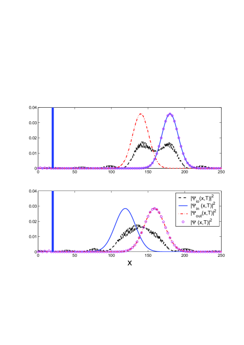
Figure 1: (Color online) Probability densities before ($t=0$) and after the collision ($t=190$) with a delta barrier. Dimensionless units with $m=\hbar=1$. The initial wave packet is $\psi(k)=N[1-\exp(-\beta k^{2})]\exp[-(k-k_{0})^{2}/(4\Delta_{k}^{2})]\exp(-ikx_{0})\theta(k)$, where $N$ is the normalization constant and $\theta$ (here) the Heaviside step function; initial wavenumber $k_{0}=-\pi/2$, $\Delta_{k}=0.045$, $\beta=1/2$; $V=20\delta(x-20)$; initial center of the wave packet $x_{0}=180$. The delta potential is rather opaque so the the outgoing packet is advanced with respect to the incoming state.

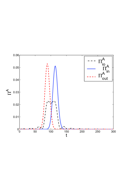
Figure 2: (Color online) Time of arrival distributions for arrivals at $x=0$ corresponding to the previous figure.

VI Application to Lyapunov operators in Quantum Mechanics

In Ref. Strauss an operator $\hat{L}$ was called a Lyapunov operator if for any normalized $|\psi\rangle$ and $|\psi_{t}\rangle\equiv e^{-i\hat{H}t/\hbar}|\psi\rangle$, the expectation value $\langle\psi_{t}|\hat{L}|\psi_{t}\rangle$ is monotonically decreasing to 0 as $t\to\infty$ and goes to 1 for $t\to-\infty$. Ref. Strauss considered the case of a Hamiltonian $\hat{H}$ with purely continuous eigenvalues ranging from 0 to infinity and degeneracy parameter $j$. The particular Lyapunov operator suggested there can be written as

$$\hat{L}_{S}=\frac{i}{2\pi\hbar}\sum_{j}\int_{0}^{\infty}dE\int_{0}^{\infty}dE^{\prime}\frac{|E,j\rangle\langle E^{\prime},j|}{E-E^{\prime}+i\varepsilon}.$$ (66)

More generally, one may call a bounded operator $\hat{L}$ a Lyapunov operator if $\langle\psi_{t}|\hat{L}|\psi_{t}\rangle$ is just monotonically decreasing, without specifying limits. However, it will be shown below, after Eq. (67), that, without loss of generality, one can always assume the above limiting behavior from 1 to 0 as $t$ goes from $-\infty$ to $+\infty$.

The above notion does not quite correspond to Lyapunov functionals used in Ref. Sewell to define irreversibility and an arrow of time, since time reversal invariance of the functional was assumed there in order to have neutrality with respect to past and future. It will be shown further below that there are no time reversal invariant Lyapunov operators if the Hamiltonian is time reversal invariant.

It is clear that the above properties do not define $\hat{L}$ in Eq. (66) uniquely. For example, one can introduce phases and still get a Lyapunov operator. In this section we are going to determine the most general form of $\hat{L}$ for a Hamiltonian $\hat{H}$ with a purely (absolutely) continuous spectrum and give conditions under which it becomes unique. It will also be seen that to each $\hat{L}$ there is an associated covariant time operator $\hat{T}_{L}$.

To show that one can assume the above limit behavior we put, for a given general Lyapunov operator $\hat{L}$,

$$\hat{L}_{t}\equiv e^{-i\hat{H}t/\hbar}\hat{L}e^{i\hat{H}t/\hbar}$$ (67)

so that $\hat{L}_{t}$ is monotonically increasing, by the monotonic decrease of $\langle\psi_{t}|\hat{L}|\psi_{t}\rangle$. From the boundedness of $\hat{L}$ and from monotonicity it follows that $\hat{L}_{\pm\infty}$ exist as operator limits in the weak sense, i.e. for expectation values. Moreover, $\hat{L}_{\pm\infty}$ commutes with $e^{-i\hat{H}t/\hbar}$, and therefore $\hat{L}^{\prime}\equiv\hat{L}-\hat{L}_{-\infty}$ is also a Lyapunov operator, with $\hat{L}^{\prime}_{t}\geq 0$. Then $\hat{L}^{\prime\prime}\equiv\hat{L}^{\prime-1/2}\hat{L}^{\prime}\hat{L}^{\prime-1/2}$ is a Lyapunov operator satisfying $\hat{L}^{\prime\prime}_{-\infty}=0$ and $\hat{L}^{\prime\prime}_{\infty}=1$ so that $\langle\psi_{t}|\hat{L}^{\prime\prime}|\psi_{t}\rangle$ is monotonically decreasing from 1 to 0, proving the above claim.

To determine the general form of $\hat{L}$ with such a limit behavior for $t\to\pm\infty$, we note that by monotonicity

$$\hat{\Pi}^{L}_{t}\equiv\frac{d}{dt}{\hat{L}}_{t}=e^{-i\hat{H}t/\hbar}\frac{-i}{\hbar}[\hat{H},\hat{L}]e^{i\hat{H}t/\hbar}\geq 0,$$ (68)

i.e. expectation values of $\dot{\hat{L}}_{t}$ are non-negative for all $t$, in particular

$$\hat{\Pi}^{L}_{0}=\frac{-i}{\hbar}[\hat{H},L]\geq 0$$ (69)

where the commutator is again to be understood in the weak sense via matrix elements and where $\hat{\Pi}^{L}_{0}$ is in general not an operator but only a bilinear form, as in Eq. (9). From Eq. (68) and from $\hat{L}_{-\infty}=0$ one obtains

$$\hat{L}=\int_{-\infty}^{0}{dt}\,e^{-i\hat{H}t/\hbar}\,\hat{\Pi}^{L}_{0}\,e^{i\hat{H}t/\hbar}.$$ (70)

From Eq. (68) one sees that

$$\Pi_{L}(t;\psi)\equiv\langle\psi|\hat{\Pi}^{L}_{t}|\psi\rangle\,\geq\,0$$ (71)

is a non-negative density which integrates to 1 for each normed state, i.e. it can be regarded as a probability density and hence $\hat{L}_{t}$ behaves like the cumulative probability operator $\hat{F}_{\tau}$ in Eq. (1). Therefore,

$$\hat{T}_{L}\equiv\int dt\,t\,e^{-i\hat{H}t/\hbar}\,\hat{\Pi}^{L}_{0}\,e^{i\hat{H}t/\hbar}$$ (72)

is an analog of the time operator $\hat{T}$ in Eq. (5). Alternatively, $1-\hat{L}_{-t}$ behaves as the cumulative arrival probability operator $\hat{F}^{A}_{t}$ in Eq. (17).
Example: Let $\hat{\Pi}^{L}_{0}$ given by Eq. (14). Then, by Eq. (70), $\hat{L}$ is given by

$$\hat{L}=\frac{1}{2\pi\hbar}\int^{0}_{-\infty}dt\int dE~{}dE^{\prime}e^{-i(E-E^{\prime})t/\hbar}|E\rangle\langle E^{\prime}|,$$ (73)

which is readily seen to agree with $\hat{L}_{S}$ in Eq. (66) in the case of non-degeneracy.

For free motion on the half-line, with $|E\rangle=|E_{f}\rangle$ from Eq. (47), the Lyapunov property of this example simply reflects the monotonous accumulation of arrivals at the origin since a change of integration variable gives

$$\langle\psi_{t}|1-\hat{L}|\psi_{t}\rangle=\int_{-\infty}^{t}dt^{\prime}\,\langle\psi|\hat{\Pi}^{0}_{f,\,t^{\prime}}|\psi\rangle.$$ (74)

With a potential on the half-line and taking $|E\rangle=|E_{\pm}\rangle$ of the previous section one obtains the accumulation of arrivals of the freely moving packets $|\psi_{in}\rangle$ and $|\psi_{out}\rangle$, and for $|E\rangle=|E_{\Theta}\rangle$ the corresponding accumulation of arrivals for $|\psi_{io}\rangle$.

The most general form of $\hat{L}$ is obtained from the most general form of $\hat{\Pi}^{L}_{0}$ which is given by Eqs. (31) and (32). If $\hat{\Pi}^{L}_{0}$ is known then $\hat{L}$ is given by Eq. (70), and in this way one obtains the most general form of the Lyapunov operator $\hat{L}$ with the above limit behavior for $t\to\pm\infty$. Uniqueness of $\hat{L}$ may be achieved for particular Hamiltonians by demanding, e.g. time reflection invariance of $\hat{T}_{l}$, special symmetries and minimal variance $\Delta T_{L}$, as in Sections IV and V.

We finally show that for a time reversal invariant Hamiltonian there is no nontrivial time reversal invariant Lyapunov operator. Indeed, if $\hat{\Theta}\,\hat{H}\,\hat{\Theta}=\hat{H}$ and $\hat{\Theta}\,\hat{L}\,\hat{\Theta}=\hat{L}$ then one obtains, for initial state $\hat{\Theta}\,|\psi\rangle\equiv|(\hat{\Theta}\psi)\rangle$,

$$\langle(\hat{\Theta}\psi)_{t}|\hat{L}|(\hat{\Theta}\psi)_{t}\rangle=\langle\psi_{-t}|\hat{L}|\psi_{-t}\rangle~{}$$ (75)

by the anti-unitarity of $\hat{\Theta}$. Now, for increasing $t$, the expression on the left-hand side decreases while the one on the right-hand side increases. This is only possible if both sides are constant in $t$. Alternatively, one can conclude from Eq. (69) that both $\hat{\Pi}^{L}_{0}$ and $\hat{\Theta}\,\hat{\Pi}^{L}_{0}\,\hat{\Theta}=-\hat{\Pi}^{L}_{0}$ are positive operators, which is only possible if $\hat{\Pi}^{L}_{0}=0$. This means that $\hat{L}$ commutes with $\hat{H}$, which also leads to the constancy of both sides in Eq. (75).

VII Discussion and outlook

We have provided the most general form of covariant, normalized time operators. This is important to set a flexible framework where physically motivated conditions on the observable may be imposed. The application examples include clock time operators, time-of-arrival operators and Lyapunov operators.

Experimentally, a number of interesting open questions remain for quantum clocks and arrival-time measurements. For example, quantum clocks are basically quantum systems with an observable that evolves linearly with time. To evaluate the possibility to compete with current atomic clocks MLM , the observable must be realized in a specific system. We have described an ideal observable (by imposing antisymmetry with respect to time reversal and minimal variance) and the analysis of the operational realization is now pending. A similar analysis for the ideal arrival time-of-arrival distribution of Kijowski has been carried out in terms of an operational quantum-optical realization with cold atoms (cf. Ref. toatqm2 for a review). Indeed, cold atoms and quantum optics offer examples of times of events (other than arrivals), such as jump times, excitation times, escape times, admitting a treatment in terms of covariant observables. Modeling and understanding these quantities and their statistics may improve our ability to manipulate or optimize dynamical processes.

On the theory side, an open question is how to adapt the proposed framework, possibly in combination with previous investigations crossstates ; Leon ; toapot ; HSMN ; Galapon06 ; Galapon08 ; Galapon , to arrival times when a particle moves in a potential.

Finally, we have shown that Lyapunov operators follow naturally from covariant time observables. Associated to time-of-arrival operators, they account for the monotonous accumulation of arrivals for freely moving asymptotic states from the infinite past independently of the state chosen. Note that the “infinite past” here is an idealized construct since it must be assumed that the wave has been evolving forever, ignoring the fact that in practice the state may have been prepared at some specific instant. In other words the Lyapunov operator does not depend on that preparation instant, and when applied to the state it takes into account its idealized (not necessarily actual) past, whether or not that past has been fully or partially realized.

We have also shown at the end of the last section that in theories with a time reversal invariant Hamiltonian there are no time reversal invariant Lyapunov operators. In Ref. Sewell it was argued that in order to characterize a system as irreversible and single out a direction of time a Lyapunov functional should be time reversal invariant. Hence, if one accepts this view of Ref. Sewell then, by our result, quantum mechanics for finitely many particles should indeed not be irreversible and should not exhibit an arrow of time if the Hamiltonian is time reversal invariant.

Appendix A Minimal variance and non-uniqueness of time operator

We show for the case of a non-degenerate spectrum of $\hat{H}$ that minimal variance alone does not imply uniqueness of $\hat{T}$. We first consider a state $|\psi\rangle$ such that, with a given choice of generalized eigenvectors, $\langle E|\psi\rangle\equiv\psi(E)$ is real. Then the first term on the r.h.s of Eq. (25) is the integral of a total derivative and therefore vanishes, as does the third term on the r.h.s. of Eq. (26), by Eq (24). Thus

$$\Delta T^{2} = \int dE\,|\psi^{\prime}|^{2}+\sum_{i}\int dE\,|b_{i}^{\prime}|^{2}\,|\psi|^{2}$$ (76)

$$- \left(\int dE\,|\psi|^{2}\,i\sum_{i}b_{i}\overline{b_{i}^{\prime}}\right)^{2}.$$

By Schwarz’s inequality the last term can be estimated as

$$\Big{|}\sum_{i}\int dE\,|\psi|^{2}\,b_{i}\,\overline{b_{i}^{\prime}}\,\Big{|}^{2}$$

$$\leq\sum_{i}\int dE\,|\psi|^{2}\,|b_{i}|^{2}\cdot\sum_{i}\int dE\,|\psi|^{2}\,|b_{i}^{\prime}|^{2},$$ (77)

where the first sum on the r.h.s. yields 1 and the equality sign holds if and only if

$$b_{i}^{\prime}(E)=\gamma\,b_{i}(E)~{}~{},~{}~{}\gamma=\mbox{constant},$$ (78)

which implies

$$\sum b_{i}\,\overline{b_{i}^{\prime}}=\bar{\gamma}\sum b_{i}\,\overline{b_{i}}=\bar{\gamma}.$$ (79)

Since the l. h. s. is purely imaginary, from Eq. (24), this implies $\gamma=i\lambda$ with $\lambda$ real. Thus, for real $\psi(E)$,

$$\Delta T^{2}\geq\int dE|\psi^{\prime}(E)|^{2},$$ (80)

with equality holding if and only if Eq. (78) holds with $\gamma=i\lambda~{},~{}\lambda$ real, i.e. if and only if

$$b_{i}(E) = c_{i}\,e^{i\lambda E}~{},~{}~{}~{}~{}\lambda~{}\mbox{real}$$ (81)

$$\sum_{i}b_{i}(E)\,\overline{b_{i}(E)} = \sum|c_{i}|^{2}=1.$$

These functions give the same time operator and density as the single function

$$b(E)=e^{i\lambda E}.$$ (82)

With this choice $\Delta T^{2}$ becomes minimal for real $\psi(E)$.

For a state given by $e^{i\varphi(E)}\psi(E)$, with real $\psi(E)$ and $\varphi(E)$, the same argument gives, upon replacing $b_{i}$ by $e^{-i\varphi(E)}\,b_{i}$, that one has minimal variance if and only if

$$b_{i}(E)=c_{i}\,e^{i(\lambda-\varphi(E))}.$$ (83)

This differs from Eq. (81), as does the analog $e^{i(\lambda-\varphi(E))}$ of the single function in Eq. (82).

Hence among the set of all allowed functions $b_{i}(E)$ there is no choice of functions such that $\Delta T$ becomes minimal for all states with finite second moment.

References

- (1) J. G. Muga, R. Sala Mayato and I. L. Egusquiza (eds.), Time in Quantum Mechanics, Vol. 1, Lect. Notes Phys. 734, Springer-Verlag, Berlin 2008.
- (2) J. G. Muga, A. Ruschhaupt and A. del Campo, Time in Quantum Mechanics, Vol. 2, Lect. Notes Phys. 789, Springer-Verlag, Berlin 2009.
- (3) A. S. Holevo, Probabilistic and statistical aspects of quantum theory, North Holland, Amsterdam, 1982.
- (4) M. J. W. Hall, eprint arXiv:0802.2682.
- (5) J. Muñoz, I. L. Egusquiza, A. del Campo, D. Seidel and J. G. Muga, Lect. Not. Phys. 789, 97 (2009).
- (6) R. Sala Mayato, D. Alonso, and I. L. Egusquiza, Lect. Notes Phys. 734, 235 (2008).
- (7) F. T. Smith, Phys. Rev. 118, 349 (1960).
- (8) Y. Strauss, J. Silman, S. Machnes, L.P. Horwitz, eprint arXiv:0802.2448.
- (9) G. L. Sewell, Quantum Mechanics and its Emergent Macrophysics, Princeton University Press, Princeton and Oxford, 2002, p. 84.
- (10) M. J. Hall, J. Phys. A: Math. Theor. 41, 255301 (2008).
- (11) S. L. Braunstein, C. M. Caves and G. J. Milburn, Ann. Phys. (NY) 247, 135 (1996).
- (12) M. J. Hall in “Quantum Communications and Measurement”, ed. by V. P. Belavkin, O. Hirota and R. L. Hudson (New York: Plenum, New York 1995) p. 53.
- (13) J. G. Muga and C. R. Leavens, Phys. Rep. 338, 353 (2000).
- (14) A. Ruschhaupt, J. G. Muga and G. C. Hegerfeldt, Lect. Not. Phys. 789, 65 (2009).
- (15) R. Werner, J. Math. Phys. 27, 793 (1986).
- (16) J. Kijowski, Rep. Math. Phys. 6, 362 (1974).
- (17) G. C. Hegerfeldt and J. G. Muga, in preparation
- (18) G. C. Hegerfeldt, D. Seidel, J. G. Muga, and B. Navarro, Phys. Rev. A 70, 012110 (2004).
- (19) J. León, J. Julve, P. Pitanga, and F. J. de Urríes, Phys. Rev. A 61, 062101 (2000).
- (20) A. D. Baute, I. L. Egusquiza and J. G. Muga, Phys. Rev. A 64, 012501 (2001).
- (21) J. Muñoz, I. Lizuain and J. G. Muga, Phys. Rev. A 80, 022116 (2009).
- (22) A. D. Baute, R. Sala Mayato, J. P. Palao, J. G. Muga and I. L. Egusquiza, Phys. Rev. A 61, 022118 (2000).
- (23) E. A. Galapon, Int. J. Mod. Phys. A 21, 6351 (2006).
- (24) E. A. Galapon and A. Villanueva, J. Phys. A:Math. Theor. 41, 455302 (2008).
- (25) E. A. Galapon, Lect. Notes Phys. 789, 25 (2009), and references therein.