User Scheduling for Cooperative Base Station Transmission Exploiting Channel Asymmetry

Abstract

We study low-signalling overhead scheduling for downlink coordinated multi-point (CoMP) transmission with multi-antenna base stations (BSs) and single-antenna users. By exploiting the asymmetric channel feature, i.e., the pathloss differences towards different BSs, we derive a metric to judge orthogonality among users only using their average channel gains, based on which we propose a semi-orthogonal scheduler that can be applied in a two-stage transmission strategy. Simulation results demonstrate that the proposed scheduler performs close to the semi-orthogonal scheduler with full channel information, especially when each BS is with more antennas and the cell-edge region is large. Compared with other overhead reduction strategies, the proposed scheduler requires much less training overhead to achieve the same cell-average data rate.

I Introduction

Base station (BS) cooperative transmission, also known as coordinated multi-point (CoMP) transmission, has received much attention for providing high spectral efficiency in cellular networks [1]. By sharing data and channel state information (CSI) among multiple BSs, CoMP-JP (joint processing) can fully exploit the benefits of the cooperation. Among various challenges such as BS synchronization, backhaul cost and channel acquisition, the overhead to gather CSI is the most limiting factor that hinders the application of CoMP.

Multi-user multi-input multi-output (MU-MIMO) techniques can exploit the abundant spatial resources in downlink CoMP-JP systems. When the number of users exceeds that of transmit antennas, spatial user scheduling becomes critical [2], which however requires enormous training or feedback overhead even in single-cell systems [3]. To reduce the overhead in case it counteracts the performance gain, the training symbol length was optimized to maximize a net throughput excluding the overhead [4]. The overhead can also be reduced by differentiating what the CSI is used for. For example, when zero-forcing beamforming (ZFBF) is employed, channel direction information is essential for beamforming, and channel norms and channel orthogonality among users are essential for a well known semi-orthogonal user scheduler (SUS) [2]. Alternatively, the overhead can be reduced by selective feedback [5] or by exploiting channel statistics [6].

Though CoMP-JP exhibits many similarities to single-cell MU-MIMO, there are distinctive differences in the channel properties and system setting. One of them is the inherent channel asymmetry of CoMP systems, i.e., the average channel gains from multiple BSs to each user are non-identical [7]. Despite that many well-explored precoders and schedulers can be directly applied for CoMP-JP systems if full CSI of all candidate users is available, such a unique channel feature can be exploited to further reduce the required overhead.

This paper aims at designing low-overhead scheduling for downlink CoMP-JP systems. Considering that SUS [2] is an asymptotically optimal low-complexity scheduler in terms of sum rate for large number of users in conjunction with ZFBF, we base our proposal on the same main principle, i.e., the users with larger channel powers will be selected if the angles between their channel directions exceed a predetermined threshold. In single-cell systems, full CSI of all candidate users is required for SUS. In CoMP systems, we show that the channel orthogonality among users largely depends on the average channel gains of the users. Based on this observation, we derive new metrics for scheduling merely using large-scale fading gains, with which a low-overhead scheduler is proposed, named large-scale fading gain based user scheduler (LargeUS). This scheduler can be applied for a two-stage transmit strategy, where in the first stage, scheduling is performed based only on the large-scale fading gains of all candidate users and in the second stage, beamforming is done using full CSI of the selected users. Despite that channel asymmetry is exploited to derive the LargeUS, simulation results show that it performs close to SUS using full CSI even when the users are located in cell-edge regions.

In [8], a channel norm-based scheduler was proposed, where the users with the largest instantaneous channel norms are selected, which however differs from our method since the proposed scheduler takes both the orthogonality and receive power into account.

Notations: Boldface upper and lower case letters denote matrices and row vectors, and standard lower case letters denote scalars. Superscripts $(\cdot)^{T}$, $(\cdot)^{H}$ and $(\cdot)^{\dagger}$ denote the transpose, the conjugate transpose and the Moore-Penrose inverse, respectively. $\Re\{\cdot\}$ and $\Im\{\cdot\}$ denote the real and imaginary parts, $\mathbb{E}\{\cdot\}$ denotes the expectation operator, and $\cup$ denotes the union between two sets. $\|\mathbf{a}\|$ denotes the Euclidean norm of a vector $\mathbf{a}$, $|\mathbf{A}|$ denotes the determinant of a matrix $\mathbf{A}$, and $\mathrm{diag}\{\mathbf{A}_{1},\dots,\mathbf{A}_{n}\}$ represents the block diagonal matrix with diagonal matrices $\mathbf{A}_{1},\dots,\mathbf{A}_{n}$. $\mathbf{x}\sim\mathcal{CN}(\mathbf{0},\boldsymbol{\Sigma})$ denotes a circularly symmetric complex Gaussian vector $\mathbf{x}$ with covariance matrix $\boldsymbol{\Sigma}$ and zero mean. $\mathbb{C}^{m\times n}$ denotes the set of all $m\times n$ complex matrices. Finally, $\mathbf{I}$ denotes the identity matrix, and $\mathbf{0}$ denotes the vector of zeros.

Acronyms used throughout the paper are listed in Table I.

[b] BS Base Station CDF Cumulative Distribution Function CoMP^$\ast$ Coordinated Multi-point CSI Channel State Information FDD Frequency Division Duplex JP Joint Processing LargeUS Large-scale fading gain based User Scheduler LTE Long Term Evolution MU-MIMO Multi-user Multi-input Multi-output NMSE Normalized Mean Square Errors OFDM Orthogonal Frequency Division Multiplexing PBPC Per-BS Power Constraints PDF Probability Density Function PF Proportional Fair RR Round Robin SFUS Selective Feedback based User Scheduler SINR Signal-to-Interference plus Noise Ratio SNR Signal-to-Noise Ratio SUS Semi-orthogonal User Scheduler TDD Time Division Duplex ZFBF Zero-forcing Beamforming

TABLE I: Acronyms

• CoMP is also used to mean CoMP-JP for notational simplicity from Section II.

II System Model

Consider one cluster of a downlink CoMP-JP system consisting of $M$ coordinated cells, each including one BS and $K$ users. Each BS is equipped with $N_{t}$ antennas and each user has a single antenna. For simplicity, we refer to CoMP-JP as CoMP in the rest of the paper.

We consider that all the $MK$ users are located in a cell-edge region. For each user, we define its local BS as the BS providing the largest receive power. The channel between a user and its local BS is called local channel, while the channels between the user and its cooperating BSs are called cross channels. We use $i_{km}$ to denote the index of the $k$th user located in cell $m$. Then for user $i_{km}$ (denoted by $\text{MS}_{i_{km}}$), its channel asymmetry is reflected by a parameter defined as $\rho_{i_{km}}=\frac{\alpha_{i_{km}m}}{\max_{n\neq m}\alpha_{i_{km}n}}$, where $\alpha_{i_{km}m}$ and $\alpha_{i_{km}n}$ for $n\neq m$ are the large-scale fading gains of local and cross channels of $\text{MS}_{i_{km}}$, respectively. The large-scale fading gains include both pathloss and shadowing. Shadowing usually follows a log-normal distribution, but we assume that $\alpha_{i_{km}n}$ is deterministic as in most works in the literature of CoMP [7] because the time scale of user scheduling is much shorter than the large-scale fading variations. If the value of $\rho_{i_{km}}$ is less than a predefined parameter $\bar{\rho}$, we say that $\text{MS}_{i_{km}}$ is located in a “$\bar{\rho}$ cell-edge region”. Fig. 1 illustrates the 3 dB and 10 dB cell-edge regions.

Let $\tilde{\mathbf{h}}_{i_{km}n}$ and $\mathbf{h}_{i_{km}n}$ denote the small-scale fading channel and the composite channel from the $n$th BS (denoted by $\text{BS}_{n}$) to $\text{MS}_{i_{km}}$, where $\mathbf{h}_{i_{km}n}=\sqrt{\alpha_{i_{km}n}}\tilde{\mathbf{h}}_{i_{km}n}\in\mathbb{C}^{1\times N_{t}}$. Then the global channel of $\text{MS}_{i_{km}}$ can be expressed as $\mathbf{h}_{i_{km}}=\left[\mathbf{h}_{i_{km}1},\dots,\mathbf{h}_{i_{km}M}\right]\in\mathbb{C}^{1\times MN_{t}}$. To focus on the impact of channel asymmetry on user scheduling, we consider flat fading channel and the small-scale fading channel follows independent and identically distributed (i.i.d.) complex Gaussian distribution, i.e., $\tilde{\mathbf{h}}_{i_{km}n}\sim\mathcal{CN}(\mathbf{0},\mathbf{I})$. Furthermore, we assume that the small-scale fading channels from different BSs to each user are independent. Then $\mathbf{h}_{i_{km}}\sim\mathcal{CN}(\mathbf{0},{\mathbf{R}}_{i_{km}})$ with ${\mathbf{R}}_{i_{km}}=\text{diag}\{\alpha_{i_{km}1}{\mathbf{I}},\dots,\alpha_{i_{km}M}{\mathbf{I}}\}$.

We consider time division duplex (TDD) CoMP systems with a two-stage transmission strategy. In the first stage, scheduling is performed using only large-scale fading gains of all the candidate users. In the second stage, the selected users are informed to provide their full CSI, with which the precoders are computed. We employ Moore-Penrose inverse based ZFBF for precoding, which is of low complexity and is widely studied [2, 9].

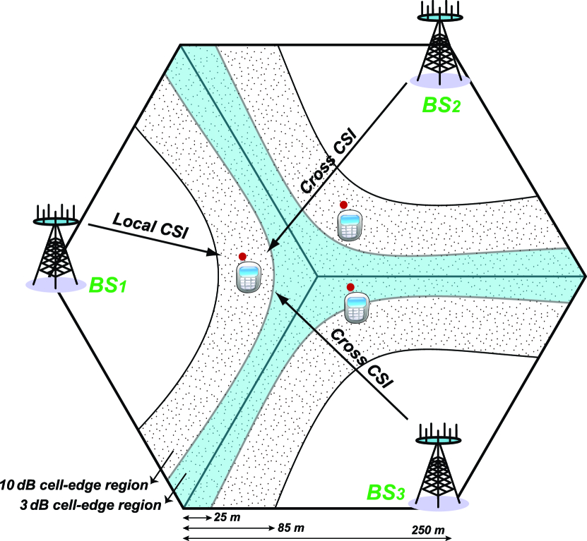
Figure 1: The layout of the reference CoMP cluster, where three BSs cooperatively serve users located in cell-edge regions, the cell radius $r$ is 250 m, and the pathloss follows $35.3+37.6\log_{10}(d)$ [10]. The 3 dB and 10 dB cell-edge regions are around 25 m and 85 m away from the cell boundary, respectively. The regular cell-edge regions are obtained without considering shadowing in order to provide an easy understanding.

III Low-overhead User Scheduler

In this section, we propose a low-overhead scheduler using the same principle as SUS by exploiting the channel asymmetry. We first show that the channel orthogonality between users can be approximately determined based on the average channel gains. Then we derive new scheduling metrics only with large-scale fading gains, from which a low-overhead scheduler is developed for CoMP systems.

III-A Probability of Orthogonality between CoMP Channels

The scheduling principle employed in SUS is as follows: the users with large receive power and with good orthogonality among each other are successively selected [2], which is called SUS principle for short in the sequel. For two users (say $\text{MS}_{1}$ and $\text{MS}_{2}$), the orthogonality between their channels can be represented by the cosine of the angle between their channel vectors $\cos\theta=\frac{|\mathbf{h}_{1}\mathbf{h}_{2}^{H}|}{\|\mathbf{h}_{1}\|\|\mathbf{h}_{2}\|}$, $0\leq\theta\leq{\pi}/{2}$. When $\cos\theta=0$, the channels of the two users are orthogonal.

We derive the probability density function (PDF) of $\cos^{2}\theta$ in Appendix A. To gain some insight, the PDF for the special case of two single-antenna coordinated BSs is given by

$$f_{\cos^{2}\theta}(x)=\int_{0}^{1} \frac{\kappa_{1}\kappa_{2}}{\left((\kappa_{1}-1)t_{1}+1\right)^{2}\left((1-\kappa_{2})\delta+\kappa_{2}\right)^{2}}$$

$$\cdot\left(1-\frac{4(\kappa_{1}-1)^{2}t_{2}}{\left((\kappa_{1}-1)t_{1}+1\right)^{2}}\right)^{-\frac{3}{2}}d\delta,$$ (1)

where $t_{1}=\delta(1-x)+(1-\delta)x$, $t_{2}=\delta(1-\delta)x(1-x)$, and $\kappa_{i}=\alpha_{i1}/\alpha_{i2}$ for $i=1,2$. When $\kappa_{i}=1$ (i.e., $0$ dB), $\text{MS}_{i}$ is located at the cell boundary and its channel is not asymmetric.

According to the results shown in [2], the cosine of the angle between channel vectors of any two selected users by SUS is less than 0.5. Therefore, we can say that $\text{MS}_{1}$ and $\text{MS}_{2}$ are semi-orthogonal when $\cos^{2}\theta<0.25$. Numerical results of the probability of $\cos^{2}\theta<0.25$ (i.e., $\theta>60^{\circ}$) are depicted in Fig. 2(a), where two users are considered. It is shown that when the channel of a user is not asymmetric, i.e., $\kappa_{1}=0$ dB, the probability that it is orthogonal with the other user’s channel is low and does not depend on the location of the other user. This implies that in single-cell systems with i.i.d. channels, we have to use full CSI to decide the channel orthogonality. When the channels of the two users are asymmetric, their orthogonality depends on the users’ location. The probability of $\theta>60^{\circ}$ is very low when two users are located in the same cell, while it becomes larger when they are in different cells. Resembling single-cell MIMO systems, when the BS has more antennas, the behavior is similar except that the users will be orthogonal with a higher probability. This indicates that we can use large-scale fading gains to decide the orthogonality between users in CoMP systems. In the following, we derive low-overhead scheduling metrics for selecting users based on the SUS principle by efficiently exploiting the large-scale fading gains.

III-B Low-overhead SUS-based Scheduler

III-B1 Scheduling Metrics with Large-scale Fading Gains

When full CSI of all candidate users is available, to decide whether $\text{MS}_{i_{km}}$ should be selected in the $(l+1)$th iteration with the SUS principle [2], we need to compute the orthogonal projection power of its channel vector on a subspace spanned by the channel vectors of already selected users, i.e.,

$$\nu_{\mathcal{S}_{l}i_{km}}=\mathbf{h}_{i_{km}}\mathbf{Q}_{\mathcal{S}_{l}}^{\bot}\mathbf{h}_{i_{km}}^{H},$$ (2)

where $\mathbf{Q}_{\mathcal{S}_{l}}^{\bot}=\mathbf{I}-\mathbf{H}_{\mathcal{S}_{l}}^{H}(\mathbf{H}_{\mathcal{S}_{l}}\mathbf{H}_{\mathcal{S}_{l}}^{H})^{\dagger}\mathbf{H}_{\mathcal{S}_{l}}$ is the orthogonal projection matrix onto the subspace spanned by $\mathbf{H}_{\mathcal{S}_{l}}$, $\mathcal{S}_{l}=\{s_{1},\dots,s_{l}\}$ is the scheduling result before the $(l+1)$th iteration, and $\mathbf{H}_{\mathcal{S}_{l}}=[\mathbf{h}_{s_{1}}^{T},\dots,\mathbf{h}_{s_{l}}^{T}]^{T}\in\mathbb{C}^{l\times MN_{t}}$ with $\mathbf{h}_{s_{i}}=[\mathbf{h}_{s_{i}1},\dots,\mathbf{h}_{s_{i}M}]\in\mathbb{C}^{1\times MN_{t}}$ for $i=1,\dots,l$. We also need to obtain the metric reflecting the orthogonality between $\text{MS}_{i_{km}}$ and already selected users in $\mathcal{S}_{l}$, which is defined as

$$\mu_{\mathcal{S}_{l}i_{km}}=\frac{\nu_{\mathcal{S}_{l}i_{km}}}{\|\mathbf{h}_{i_{km}}\|^{2}}.$$ (3)

According to the SUS principle, $\text{MS}_{i_{km}}$ will be selected if $\mu_{\mathcal{S}_{l}i_{km}}$ is larger than a specific orthogonal threshold and $\nu_{\mathcal{S}_{l}i_{km}}$ is larger than those of other candidate users.

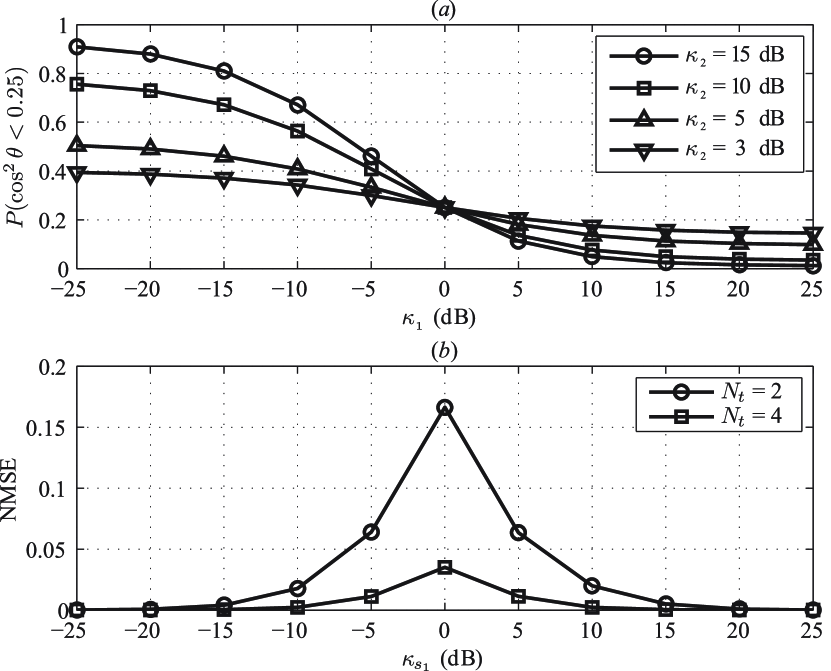
Figure 2: $(a)$ The probability of $\cos^{2}\theta<0.25$ (i.e., $\theta>60^{\circ}$) as a function of $\kappa_{1}$ in dB with $N_{t}=1$. $\text{MS}_{1}$ and $\text{MS}_{2}$ are two arbitrary users located in two cooperative cells. $\text{MS}_{i}$ is located in cell 1 if $\kappa_{i}>0$ dB and in cell 2 if $\kappa_{i}<0$ dB. $(b)$ The NMSE between $\nu_{\mathcal{S}_{l}i_{km}}$ and its approximation $\nu_{\mathcal{S}_{l}i_{km}}^{app}$ as a function of $\kappa_{s_{1}}$ with $N_{t}=2,4$, where $\mathcal{S}_{l}$ includes only one already selected user $\text{MS}_{s_{1}}$ and $\text{MS}_{i_{km}}$ is an arbitrary candidate user uniformly distributed in two cells. The results are averaged over 10000 small-scale Rayleigh fading channels following complex Gaussian distribution $\mathcal{CN}(\mathbf{0},\mathbf{I})$.

When only large-scale fading gains are available, the scheduling metrics $\mu_{\mathcal{S}_{l}i_{km}}$ and $\nu_{\mathcal{S}_{l}i_{km}}$ cannot be used any more.

To derive the metrics only dependent on average channel gains, we take the expectation of $\nu_{\mathcal{S}_{l}i_{km}}$ over the unknown small-scale channels. However, the expectation of $\nu_{\mathcal{S}_{l}i_{km}}$ is very hard to derive, because the global channel is non-identically distributed due to the channel asymmetry even when the channel from each BS is i.i.d.. To circumvent this problem, we first provide an approximation of $\nu_{\mathcal{S}_{l}i_{km}}$ by exploiting the channel asymmetry. In particular, considering that the cross channels have smaller average gains than local channels, we approximate the cross channels of the already selected users in $\mathcal{S}_{l}$ as zeros. Then the matrix $\mathbf{H}_{\mathcal{S}_{l}}$ can be approximated as a sparse matrix, denoted by $\mathbf{H}_{\mathcal{S}_{l}}^{app}\in\mathbb{C}^{l\times MN_{t}}$. By performing row interchange operations on the sparse matrix, we can obtain a block-diagonal matrix, i.e.,

$$\mathbf{\hat{H}}_{\mathcal{S}_{l}}=\boldsymbol{\Gamma}_{\mathcal{S}_{l}}\mathbf{H}^{app}_{\mathcal{S}_{l}}\triangleq\text{diag}\{\mathbf{H}_{\mathcal{S}_{l},1},\dots,\mathbf{H}_{\mathcal{S}_{l},M}\},$$ (4)

where $\boldsymbol{\Gamma}_{\mathcal{S}_{l}}\in\mathbb{C}^{l\times l}$ is the row permutation matrix satisfying $\boldsymbol{\Gamma}_{\mathcal{S}_{l}}^{H}\boldsymbol{\Gamma}_{\mathcal{S}_{l}}=\mathbf{I}$. Let $I_{\mathcal{S}_{l},n}$ denote the number of already selected users that are located in cell $n$. Then the diagonal block of $\mathbf{\hat{H}}_{\mathcal{S}_{l}}$, $\mathbf{H}_{\mathcal{S}_{l},n}$, has the dimension of $I_{\mathcal{S}_{l},n}\times N_{t}$, and consists of local channels of the $I_{\mathcal{S}_{l},n}$ selected users located in cell $n$ for $n=1,\dots,M$.

Example: Consider that two cells are coordinated and three users in $\mathcal{S}_{l}=\{s_{1},s_{2},s_{3}\}$ are successively scheduled, i.e., $M=2$ and $l=3$. Suppose that the first user $\text{MS}_{s_{1}}$ and the third user $\text{MS}_{s_{3}}$ are located in cell 2, and the second user $\text{MS}_{s_{2}}$ is located in cell 1. Then, $I_{\mathcal{S}_{l},1}=1$ and $I_{\mathcal{S}_{l},2}=2$. Following the definition of $\mathbf{H}_{\mathcal{S}_{l}}$ after (2), we have

$$\mathbf{H}_{\mathcal{S}_{l}}=\left[\mmatrix\mathbf{h}_{s_{1}1}&\underline{\mathbf{h}_{s_{1}2}}\\ \underline{\mathbf{h}_{s_{2}1}}\mathbf{h}_{s_{2}2}\\ \mathbf{h}_{s_{3}1}\underline{\mathbf{h}_{s_{3}2}}\right]\in\mathbb{C}^{3\times 2N_{t}},$$

where the local channel of each scheduled user is underlined. Then the approximation of $\mathbf{H}_{\mathcal{S}_{l}}$, $\mathbf{H}_{\mathcal{S}_{l}}^{app}$, can be obtained by omitting the cross channels of the scheduled users as

$$\mathbf{H}_{\mathcal{S}_{l}}\approx\mathbf{H}_{\mathcal{S}_{l}}^{app}=\left[\mmatrix\mathbf{0}&\underline{\mathbf{h}_{s_{1}2}}\\ \underline{\mathbf{h}_{s_{2}1}}\mathbf{0}\\ \mathbf{0}\underline{\mathbf{h}_{s_{3}2}}\right]\in\mathbb{C}^{3\times 2N_{t}}.$$

Further by performing row interchange operations on $\mathbf{H}_{\mathcal{S}_{l}}^{app}$, we obtain the block-diagonal matrix

$$\mathbf{\hat{H}}_{\mathcal{S}_{l}}=\boldsymbol{\Gamma}_{\mathcal{S}_{l}}\mathbf{H}_{\mathcal{S}_{l}}^{app}=\left[\mmatrix\underline{\mathbf{h}_{s_{2}1}}&\mathbf{0}\\ \mathbf{0}\underline{\mathbf{h}_{s_{1}2}}\\ \mathbf{0}\underline{\mathbf{h}_{s_{3}2}}\right]\in\mathbb{C}^{3\times 2N_{t}},$$

where $\boldsymbol{\Gamma}_{\mathcal{S}_{l}}=\left[\begin{smallmatrix}0&1&0\\ 1&0&0\\ 0&0&1\end{smallmatrix}\right]$ is a row permutation matrix, and the two diagonal blocks $\mathbf{H}_{\mathcal{S}_{l},1}=\mathbf{h}_{s_{2}1}$ and $\mathbf{H}_{\mathcal{S}_{l},2}=\left[\begin{smallmatrix}\mathbf{h}_{s_{1}2}\\ \mathbf{h}_{s_{3}2}\end{smallmatrix}\right]$, which have the dimension of $1\times N_{t}$ and $2\times N_{t}$, respectively.   $\Box$

Since $\mathbf{H}_{\mathcal{S}_{l}}\approx\mathbf{H}_{\mathcal{S}_{l}}^{app}$, we obtain from (4) that $\mathbf{H}_{\mathcal{S}_{l}}\approx\boldsymbol{\Gamma}_{\mathcal{S}_{l}}^{H}\mathbf{\hat{H}}_{\mathcal{S}_{l}}$. Therefore $\nu_{\mathcal{S}_{l}i_{km}}$ in (2) can be approximated as

$$\nu_{\mathcal{S}_{l}i_{km}}\approx\mathbf{h}_{i_{km}}\left(\mathbf{I}-\mathbf{\hat{H}}_{\mathcal{S}_{l}}^{H}\boldsymbol{\Gamma}_{\mathcal{S}_{l}}(\boldsymbol{\Gamma}_{\mathcal{S}_{l}}^{H}\mathbf{\hat{H}}_{\mathcal{S}_{l}}\mathbf{\hat{H}}_{\mathcal{S}_{l}}^{H}\boldsymbol{\Gamma}_{\mathcal{S}_{l}})^{\dagger}\boldsymbol{\Gamma}_{\mathcal{S}_{l}}^{H}\mathbf{\hat{H}}_{\mathcal{S}_{l}}\right)\mathbf{h}_{i_{km}}^{H}$$

$$=\|\mathbf{h}_{i_{km}}\|^{2}-\sum_{n=1}^{M}\mathbf{h}_{i_{km}n}\mathbf{H}_{\mathcal{S}_{l},n}^{H}\left(\mathbf{H}_{\mathcal{S}_{l},n}\mathbf{H}_{\mathcal{S}_{l},n}^{H}\right)^{\dagger}\mathbf{H}_{\mathcal{S}_{l},n}\mathbf{h}_{i_{km}n}^{H}$$

$$\triangleq\nu_{\mathcal{S}_{l}i_{km}}^{app}.$$ (5)

The accuracy of the approximation is shown in Fig. 2(b). Considering the case of $M=2$ and $l=1$, we evaluate the normalized mean square errors (NMSE) between $\nu_{\mathcal{S}_{l}i_{km}}$ and $\nu_{\mathcal{S}_{l}i_{km}}^{app}$, defined as $\mathbb{E}\{|\nu_{\mathcal{S}_{l}i_{km}}^{app}-\nu_{\mathcal{S}_{l}i_{km}}|^{2}\}/\mathbb{E}\{|\nu_{\mathcal{S}_{l}i_{km}}|^{2}\}$, as a function of the location of the already selected user $\text{MS}_{s_{1}}$, where $\text{MS}_{i_{km}}$ is an arbitrary candidate user uniformly distributed in the two cells. It can be seen from the simulation results that the largest NMSE occurs when $\kappa_{s_{1}}=0$ dB, i.e., the global channel of $\text{MS}_{s_{1}}$ is symmetric so that it can be regarded as a single-cell channel with $MN_{t}$ antennas. The NMSE rapidly decreases when the CoMP channel of the selected user becomes asymmetric. For instance, compared with the largest NMSE at $\kappa_{s_{1}}=0$ dB when $N_{t}=2$, over 60% reduction of NMSE can be observed at $\kappa_{s_{1}}=\pm 5$ dB. This indicates that the approximation is still sufficiently accurate when the users are located in cell-edge regions, where the difference between the local and cross channel gains is not large. Moreover, the accuracy of the approximation improves with the increase of antenna number $N_{t}$. This can be explained as follows. To obtain $\nu_{\mathcal{S}_{l}i_{km}}^{app}$, the approximation is made only for the channel matrix of already selected users $\mathbf{H}_{\mathcal{S}_{l}}$ but not for the channel of candidate user $\mathbf{h}_{i_{km}}$. According to the SUS principle, the first selected users should have large receive power and be more orthogonal among each other. This implies that these users are relatively close to their local BSs. As a result, their cross channels can be approximated as zeros and the subspace spanned by $\mathbf{H}_{\mathcal{S}_{l}}$ can be approximated by that spanned by $\hat{\mathbf{H}}_{\mathcal{S}_{l}}$. Since when each BS has more antennas the channels will on average become more orthogonal, the approximation is more accurate when $N_{t}$ increases.

We next derive the expectation of $\nu_{\mathcal{S}_{l}i_{km}}^{app}$ over unknown small-scale channels. In (III-B1), the term $\mathbf{H}_{\mathcal{S}_{l},n}^{H}\left(\mathbf{H}_{\mathcal{S}_{l},n}\mathbf{H}_{\mathcal{S}_{l},n}^{H}\right)^{\dagger}\mathbf{H}_{\mathcal{S}_{l},n}$ is a projection matrix. Therefore, considering $\mathbf{h}_{i_{km}n}\sim\mathcal{CN}(\mathbf{0},\alpha_{i_{km}n}\mathbf{I})$, it is readily obtained that

$$\mathbb{E}\left\{\mathbf{h}_{i_{km}n}\mathbf{H}_{\mathcal{S}_{l},n}^{H}\left(\mathbf{H}_{\mathcal{S}_{l},n}\mathbf{H}_{\mathcal{S}_{l},n}^{H}\right)^{\dagger}\mathbf{H}_{\mathcal{S}_{l},n}\mathbf{h}_{i_{km}n}^{H}\right\}$$

$$=\begin{cases}I_{\mathcal{S}_{l},n}\alpha_{i_{km}n}&\text{if $I_{\mathcal{S}_{l},n}<N_{t}$,}\\ N_{t}\alpha_{i_{km}n}&\text{if $I_{\mathcal{S}_{l},n}\geq N_{t}$.}\end{cases}$$

Further considering that $\mathbb{E}\{\|\mathbf{h}_{i_{km}}\|^{2}\}=N_{t}\sum_{n=1}^{M}\alpha_{i_{km}n}$, the expectation of $\nu_{\mathcal{S}_{l}i_{km}}^{app}$ can be obtained as

$$\mathbb{E}\{\nu_{\mathcal{S}_{l}i_{km}}^{app}\}=\sum_{n=1}^{M}(N_{t}-I_{\mathcal{S}_{l},n})^{+}\alpha_{i_{km}n}\triangleq\bar{\nu}_{\mathcal{S}_{l}i_{km}}^{app},$$ (6)

where $(x)^{+}=\max(x,0)$.

The metric to reflect orthogonality only using large-scale fading gains can also be derived. By replacing $\nu_{\mathcal{S}_{l}i_{km}}$ and $\|\mathbf{h}_{i_{km}}\|^{2}$ in (3) with their expectations, we obtain the metric as

$$\bar{\mu}_{\mathcal{S}_{l}i_{km}}^{app}=\frac{\bar{\nu}_{\mathcal{S}_{l}i_{km}}^{app}}{N_{t}\sum_{n=1}^{M}\alpha_{i_{km}n}}.$$ (7)

The scheduling metrics $\bar{\nu}_{\mathcal{S}_{l}i_{km}}^{app}$ and $\bar{\mu}_{\mathcal{S}_{l}i_{km}}^{app}$ depend on the locations of already selected users. We take an example to illustrate the effectiveness of using the metric of $\bar{\nu}_{\mathcal{S}_{l}i_{km}}^{app}$ for scheduling in CoMP systems. We apply the SUS principle by using $\bar{\nu}_{\mathcal{S}_{l}i_{km}}^{app}$ in a scenario of two-cell CoMP. Let $\text{MS}_{0}$ be the first selected user, and $\text{MS}_{1}$ and $\text{MS}_{2}$ be the two candidate users in the second iteration satisfying semi-orthogonal constraints. Assume that $\text{MS}_{1}$ and $\text{MS}_{2}$ are symmetrically located in cell 1 and cell 2, i.e., they have the same average local channel gains $\alpha_{11}=\alpha_{22}\triangleq\alpha_{L}$ and cross channel gains $\alpha_{12}=\alpha_{21}\triangleq\alpha_{C}$, where $\alpha_{L}>\alpha_{C}$. Then if $\text{MS}_{0}$ is located in cell 2, we can obtain from (6) that $\bar{\nu}_{\mathcal{S}_{l}1}^{app}=N_{t}\alpha_{L}+(N_{t}-1)\alpha_{C}$ and $\bar{\nu}_{\mathcal{S}_{l}2}^{app}=(N_{t}-1)\alpha_{L}+N_{t}\alpha_{C}$. So $\text{MS}_{1}$ located in different cell from $\text{MS}_{0}$ will be the second selected user since $\bar{\nu}_{\mathcal{S}_{l}1}^{app}>\bar{\nu}_{\mathcal{S}_{l}2}^{app}$. The result is consistent with the observation from Fig. 2(a) that the users in different cells are more orthogonal, which should be scheduled simultaneously. Note that channel asymmetry is essential for the effectiveness of the metric. Otherwise, if $\alpha_{L}=\alpha_{C}$ in the example, $\bar{\nu}_{\mathcal{S}_{l}1}^{app}$ will equal to $\bar{\nu}_{\mathcal{S}_{l}2}^{app}$. Then the scheduler cannot judge which user should be selected from the metric.

III-B2 Low-overhead Scheduler

With the scheduling metrics ${\bar{\nu}}_{\mathcal{S}_{l}i_{km}}^{app}$ and ${\bar{\mu}}_{\mathcal{S}_{l}i_{km}}^{app}$, we propose a low-overhead large-scale fading gain based user scheduler (LargeUS) based on the SUS principle, which operates as follows.

1. Select the user with the maximum average channel gain normalized by noise as the first user, i.e.,

   $$s_{1}=\arg\underset{i_{km}\in\mathcal{T}_{0}}{\max}~{}\frac{{N_{t}\sum_{n=1}^{M}\alpha_{i_{km}n}}}{\sigma_{i_{km}}^{2}},$$ (8)

   where $\sigma_{i_{km}}^{2}$ is the variance of noise and $\mathcal{T}_{0}=\{1,2,\ldots,MK\}$. Let $\mathcal{T}_{l}$ and $\mathcal{S}_{l}$ denote the user pool and the scheduling result at the $l$th step, and set $\mathcal{S}_{1}=\{s_{1}\}$ and $l=1$.

2. When $l\leq\min(MN_{t},MK)$, obtain the user pool as

   $$\mathcal{T}_{l}=\big{\{}i_{km}\in\mathcal{T}_{l-1},i_{km}\notin\mathcal{S}_{l}\ |\ {\bar{\mu}}_{\mathcal{S}_{l}i_{km}}^{app}\geq 1-\epsilon\big{\}},$$ (9)

   where $\epsilon$ is a specific orthogonality threshold. If $\mathcal{T}_{l}=\phi$   (empty set), the iteration will stop. Otherwise, compute ${\bar{\nu}}_{\mathcal{S}_{l}i_{km}}^{app}$ and select the new user as

   $$s_{l+1}=\arg\underset{i_{km}\in\mathcal{T}_{l}}{\max}~{}\frac{{\bar{\nu}}_{\mathcal{S}_{l}i_{km}}^{app}}{\sigma_{i_{km}}^{2}}.$$ (10)

   Set $\mathcal{S}_{l+1}=\mathcal{S}_{l}\cup\{s_{l+1}\}$ and $l=l+1$. $\qquad\qquad\qquad\ \ \square$

As mentioned before, LargeUS is applicable for a two-stage transmission strategy. After scheduling among all candidate users with their average channel gains in the first stage, the selected users are informed to provide full CSI for precoding in the second stage. Since only large-scale fading gains are required for LargeUS, which can be obtained either by long-term feedback from users or by averaging over past received signals at the BSs, uplink training is only necessary for precoding during the second stage.

In the precoding stage, the Moore-Penrose inverse based ZFBF [2] is employed for downlink transmission to the co-scheduled users in the same time and frequency resources. Let $\mathcal{S}_{L}=\{s_{1},\dots,s_{L}\}$ denote the $L$ finally scheduled users. For $\text{MS}_{s_{l}}$, its precoding vector is comprised of a unit norm beamforming vector $\mathbf{w}_{s_{l}}$ and the transmit power $p_{s_{l}}$. The beamforming vector can be expressed as

$$\mathbf{w}_{s_{l}}=\frac{\mathbf{h}_{s_{l}}\mathbf{Q}_{\mathcal{S}_{\bar{l}}}^{\bot}}{\|\mathbf{h}_{s_{l}}\mathbf{Q}_{\mathcal{S}_{\bar{l}}}^{\bot}\|},$$ (11)

where $\mathcal{S}_{\bar{l}}=\{j\in\mathcal{S}_{L},j\neq s_{l}\}$ includes all selected users except for $\text{MS}_{s_{l}}$, and $\mathbf{Q}_{\mathcal{S}_{\bar{l}}}^{\bot}$ is the orthogonal projection matrix onto the subspace spanned by the channels of users in $\mathcal{S}_{\bar{l}}$. Since power cannot be shared among coordinated BSs, the per-BS power constraint (PBPC) should be satisfied for power allocation. Given the beamforming vectors $\mathbf{w}_{s_{l}}$, the optimal power allocation $p_{s_{l}}$, aimed at maximizing sum rate, can be numerically obtained by using the method in [9].

III-B3 Threshold Selection

We next discuss the selection of orthogonality threshold $\epsilon$ by analyzing its impact on performance. To connect the threshold selection with the performance, the effective channel gain of $\text{MS}_{s_{l}}$ normalized by noise was considered in [2], which is

$$\gamma_{s_{l}}=\frac{|\mathbf{h}_{s_{l}}\mathbf{w}_{s_{l}}^{H}|^{2}}{\sigma_{s_{l}}^{2}}=\frac{\mathbf{h}_{s_{l}}\mathbf{Q}_{\mathcal{S}_{\bar{l}}}^{\bot}\mathbf{h}_{s_{l}}^{H}}{\sigma_{s_{l}}^{2}}.$$ (12)

Since we use average channel gains for scheduling, we need to employ the average normalized effective channel gain, which can be obtained from (2), (III-B1) and (6) as

$$\mathbb{E}\{\gamma_{s_{l}}\}\approx\frac{\sum_{n=1}^{M}(N_{t}-I_{\mathcal{S}_{\bar{l}},n})^{+}\alpha_{s_{l}n}}{\sigma_{s_{l}}^{2}}.$$ (13)

The orthogonality threshold $\epsilon$ has an intertwined impact on the performance. On one hand, $\mathbb{E}\{\gamma_{s_{l}}\}$ increases with the decrease of the number of selected users $I_{\mathcal{S}_{\bar{l}},n}$. Therefore, a small threshold $\epsilon$ is preferred to reduce the size of the user pool as shown in (9). On the other hand, multiuser diversity gain achieved by exploiting the large-scale channel difference among users depends on the size of $\mathcal{T}_{l-1}$, from which $\text{MS}_{s_{l}}$ is selected. Hence a sufficiently large threshold should be chosen to ensure a large user pool. We will evaluate the impact of $\epsilon$ via simulations in Section IV.

III-B4 Training Overhead

Compared with SUS that requires full CSI, the proposed scheduler needs only large-scale fading gains.

For a TDD CoMP system, by exploiting uplink-downlink channel reciprocity, the BSs can obtain the total $MN_{t}$ downlink channel coefficients from $M$ BSs to one user when the user broadcasts a single uplink training signal. Therefore, in order to obtain the full global channels of all $MK$ users for SUS, the orthogonal (in frequency, time or code domain) training sequences employed by the system require $MK$-dimensional resources. For LargeUS, the users are scheduled only using large-scale fading gains, which can be estimated by each user and fed back to its local BS. The overhead for conveying the long-term information is negligible. Alternatively, they can also be estimated at the BSs by averaging over the received signals. The uplink training is only used for estimating the full global channels of $L$ scheduled users for precoding in the second stage, which requires $L$-dimensional resources.

It should be pointed out that at the system level, the reduction of the overall uplink training overhead achieved by the proposed scheduler depends on the number of users participating CoMP transmission. The overall gain will be significant if the cells are densely deployed such that most users prefer to be served with CoMP.

IV Simulation Results

We evaluate the performance of the proposed scheduler via simulations. We consider a homogeneous cellular network and focus on the performance of a reference cooperative cluster consisting of three coordinated cells. We model the interference from surrounding non-cooperative cells as white noise, which is the worst-case interference and results in pessimistic performance [11]. The layout of the reference cooperative cluster is shown in Fig. 1. In each cell $K=10$ users are uniformly distributed in a $\bar{\rho}$ cell-edge region, where $\bar{\rho}=3$ dB and 10 dB are considered in simulations. The cell radius $r$ is set to 250 m, and the average receive signal-to-noise ratio (SNR) of the users located at cell boundary, $\text{SNR}_{0}$, is set to 0 dB and 10 dB. The average receive SNR of a user from a BS with distance $d$ is computed as $\text{SNR}_{0}+37.6\log_{10}(\frac{r}{d})$. In order to obtain regular cell-edge regions that are easy to understand, shadowing is not considered in simulations. Since shadowing enhances channel asymmetry, the analysis results are valid for practical channels with shadowing. The spatially correlated small-scale fading channels are considered based on the “Spatial Channel Model” (SCM) in urban macro scenario with four-wavelength antenna spacing and two-degree angle spread at each BS [12]. Although this model produces frequency selective channels, we consider a frequency-flat version of the channel corresponding to a single subcarrier in a subband of an orthogonal frequency division multiplexing (OFDM) system. For the scenarios when the subband width is less than the coherence bandwidth of the channel, the performance over a single subcarrier can stand for that over a subband. The subbands in a CoMP OFDM system will be orthogonal with the assumption of perfect time-frequency synchronization among the coordinated BSs. The scheduling and precoding on different subbands can be separately conducted, therefore the obtained results can reflect the performance of general OFDM systems.

Fairness among users is critical for CoMP systems, which can be ensured by either Round-Robin (RR) scheduling or proportional fair (PF) scheduling when full CSI is available. With only large-scale fading gains, however, applying PF scheduling is not straightforward because it requires the estimation of user data rate. In the simulations, we apply LargeUS in a RR fashion similar to [2], named RR-LargeUS. Specifically, it selects a group of users at each time slot based on LargeUS, and removes the selected users from the user pool at next time slot. This procedure is repeated until no users are left. As a performance baseline, SUS with full CSI in a RR fashion (denoted by RR-SUS) is simulated for both CoMP and non-CoMP systems. For comparison, we also simulate the selective feedback based user scheduler (SFUS) in a RR fashion (denoted by RR-SFUS), which will be described in detail later. We use achievable data rate as performance metric and employ ZFBF for all schemes. With ZFBF, the achievable data rate of $\text{MS}_{s_{l}}$ can be obtained as $\log(1+\frac{p_{s_{l}}|\mathbf{h}_{s_{l}}\mathbf{w}_{s_{l}}^{H}|^{2}}{\sigma_{s_{l}}^{2}})$, where $\mathbf{w}_{s_{l}}$ is the beamforming vector defined in (11) and $p_{s_{l}}$ is the power allocated to $\text{MS}_{s_{l}}$ that is optimized aimed at maximizing the achievable sum rate under PBPC [9].

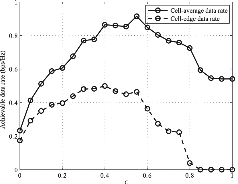
Figure 3: Cell-average and cell-edge data rate of RR-LargeUS as a function of threshold $\epsilon$ with $N_{t}=4$ and $\text{SNR}_{0}=10$ dB. The users are located in a 10 dB cell-edge region.

In Fig. 3, we plot the cell-average data rate and the cell-edge data rate achieved by the proposed scheduler versus the threshold $\epsilon$ with $N_{t}=4$ and $\text{SNR}_{0}=10$ dB. The cell-average data rate is the average achievable data rate of all users, and the cell-edge data rate is defined as the 5% point of the cumulative distribution function (CDF) of user achievable data rate. As can be seen, the data rate is not a monotonic function of the threshold. This agrees with the previous analysis of the influence of the threshold both on the effective channel gain and on the multiuser diversity gain. The curves are not smooth because of the discontinuous changes of the RR scheduling period. Since the users are served only once during a RR scheduling period, their data rate is normalized by the period. For a given number of total users, the scheduling period depends on the number of selected users at each time slot [2], which is determined by the threshold. We can see that the optimal thresholds for maximum cell-average and cell-edge data rate differ. This is due to the fact that the orthogonality among users depends on their locations. In the following simulations we will choose the thresholds that provide a balance between high cell-average and cell-edge data rate, which values are given in the figure captions.

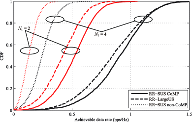
(a) 3 dB cell-edge region

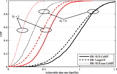
(b) 10 dB cell-edge region

Figure 4: The CDF of user data rate for various cell-edge regions with $N_{t}=2,4$ and $\text{SNR}_{0}=10$ dB. The thresholds $\epsilon$ for RR-SUS and RR-LargeUS are chosen as 0.6 and 0.55, respectively, which are also used in Fig. 6. The legends “RR-SUS CoMP” and “RR-SUS non-CoMP” respectively stand for RR-SUS under CoMP and non-CoMP systems, all with full CSI.

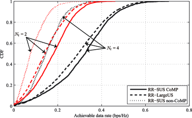
(a) 3 dB cell-edge region

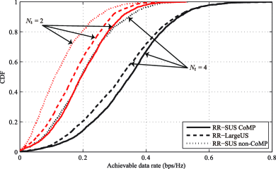
(b) 10 dB cell-edge region

Figure 5: The CDF of user data rate for various cell-edge regions with $N_{t}=2,4$ and $\text{SNR}_{0}=0$ dB. The thresholds $\epsilon$ for RR-SUS and RR-LargeUS are chosen as 0.5 and 0.45, respectively, which are also used in Fig. 7. The legends “RR-SUS CoMP” and “RR-SUS non-CoMP” respectively stand for RR-SUS under CoMP and non-CoMP systems, all with full CSI.

Figure 4 shows the CDF of user data rate achieved by LargeUS and SUS with $N_{t}=2,4$ and $\text{SNR}_{0}=10$ dB, where 3 dB and 10 dB cell-edge regions are considered, respectively. Compared to non-CoMP systems, CoMP transmission provides an evident performance gain as expected. In CoMP systems, the performance gap between RR-LargeUS and RR-SUS decreases when $N_{t}$ increases from 2 to 4. This is because more antennas can improve the accuracy of the approximation used in deriving the scheduling metrics as shown in Fig. 2(b). For large cell-edge regions, the approximation is accurate, also as shown in Fig. 2(b). Consequently, we can see from Fig. 4(b) that RR-LargeUS performs close to RR-SUS. For small cell-edge regions, the channels become not so asymmetric that the approximation is not very accurate. Although this will lead to performance degradation for RR-LargeUS, Fig. 4(a) shows that the performance loss compared to RR-SUS is small when $N_{t}=4$. Similar results at $\text{SNR}_{0}=0$ dB can be observed in Fig. 5, but the performance gain of CoMP over non-CoMP reduces because the systems become noise-limited.

Finally, we compare the cell-average data rate of the low-overhead RR-SFUS and the relevant schedulers with $N_{t}=4$ in Fig. 6 and Fig. 7, where $\text{SNR}_{0}$ is set to 10 dB and 0 dB, respectively. Based on the idea of reducing feedback overhead for frequency division duplex (FDD) systems proposed in [5], in TDD systems RR-SFUS can operate as follows.

1. Channel acquisition: The coordinated BSs need to know at least full local channels of all users. In addition, the full cross channels with large receive power also need to be provided to BSs. Let $\psi$ denote the ratio of the number of selected channel coefficients to global channels. Then, we have $\frac{1}{M}\leq\psi\leq 1$. The value of $\psi$ depends on a predetermined receive power threshold [5], by adjusting which we consider different $\psi$ in Fig. 6 and Fig. 7.

2. Scheduling: With the incomplete CSI (the cross channels with lower receive power are set to zeros), RR-SFUS schedules users by using the method of SUS in a RR fashion. Note that a scheduler was proposed for the selective feedback strategy in [5] but aimed at reducing backhauling loads and hence is not suitable for our considered scenario.

3. Precoding: Based on the types of CSI used for precoding, two RR-SFUS strategies are considered as follows:

   • RR-SFUS-1: The same incomplete CSI for scheduling, including full local CSI and some full cross CSI, is used for ZFBF precoding. Therefore, in this case both scheduling and precoding are performed in one stage (denoted by RR-SFUS-1). Since the precoder is computed based on incomplete global channels, RR-SFUS-1 cannot thoroughly eliminate the inter-cell interference.

   • RR-SFUS-2: As an alternative, RR-SFUS can also be applied for a two-stage transmission strategy (denoted by RR-SFUS-2), where in the first stage, RR-SFUS is performed based on the incomplete global channels and in the second stage, ZFBF precoder is computed with full CSI of the selected users.

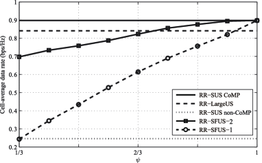
(a) 3 dB cell-edge region

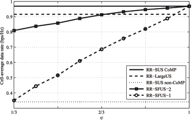
(b) 10 dB cell-edge region

Figure 6: Cell-average data rate of RR-SFUS as a function of $\psi$ for various cell-edge regions with $N_{t}=4$ and $\text{SNR}_{0}=10$ dB. RR-SFUS schedules users using SUS with full local CSI and some full cross CSI with large receive power of all candidate users, where the thresholds $\epsilon$ are properly chosen for different $\psi$. After scheduling, the ZFBF precoder is computed based on either the same incomplete CSI as scheduling (denoted by “RR-SFUS-1” in the legend) or full global channels of the selected users (denoted by “RR-SFUS-2”).

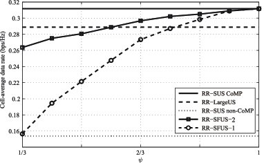
(a) 3 dB cell-edge region

(b) 10 dB cell-edge region

Figure 7: Cell-average data rate of RR-SFUS as a function of $\psi$ for various cell-edge regions with $N_{t}=4$ and $\text{SNR}_{0}=0$ dB. RR-SFUS schedules users using SUS with full local CSI and some full cross CSI with large receive power of all candidate users, where the thresholds $\epsilon$ are properly chosen for different $\psi$. After scheduling, the ZFBF precoder is computed based on either the same incomplete CSI as scheduling (denoted by “RR-SFUS-1” in the legend) or full global channels of the selected users (denoted by “RR-SFUS-2”).

We can see from Fig. 6 that RR-SFUS-1 suffers significant performance loss compared to RR-SFUS-2. To achieve the same performance as RR-LargeUS, around 90% of the channel coefficients need to be provided to the BSs for all considered cell-edge regions. The performance gap between RR-SFUS-2 and RR-LargeUS when $\psi=1/3$ reflects the importance of using large-scale gains of cross channels, which are effectively used in the scheduling metrics of RR-LargeUS but not in RR-SFUS-2. In this case, RR-SFUS-2 exploits only local channels and regards cross channels as zeros, which is equivalent to assume that the users in different cells are spatially separated. Yet, this is far from the reality as shown in Fig. 2(a). To recover the performance gap, more channel coefficients need to be provided for RR-SFUS-2. The amount increases with the shrinking of cell-edge region, e.g., 2/3 channel coefficients need to be provided for a 10 dB cell-edge region. Similar results have been observed for the cell-edge data rate, which are not shown due to space limitations. Fig. 7 considers a noise-limited scenario with $\text{SNR}_{0}=0$ dB. It can be observed that almost half of channel coefficients are required by RR-SFUS-2 to achieve the performance of the proposed LargeUS for a 10 dB cell-edge region, and even more are required for a 3 dB cell-edge region.

It is well understood that RR-SFUS can reduce the feedback overhead of FDD systems by not feeding back the weak cross channels. In the considered TDD systems, according to the principle of FDD systems, only local channel and some strong cross channels of each user need to be estimated, while some weak cross channels can be simply set to zeros. However, uplink training design for estimating a part of channel coefficients of global channels has not been well addressed so far. Thereby we cannot exactly measure the overhead of RR-SFUS-2. In general, nevertheless, the training overhead increases with a growing number of channel coefficients to be estimated, which is determined by $\psi$. This suggests that the training overhead is maximal when $\psi=1$, i.e., estimating full global channels of all candidate users, which is $MK$-dimensional resources as explained in Section III-B4. The lower bound of the training overhead can be obtained when $\psi=1/3$. In this case, the BSs only estimate local channels of all candidate users for scheduling in the first stage. The training overhead is the same as that in non-CoMP systems, which needs $K$-dimensional resources. In the second stage, $L$-dimensional resources are used to estimate full global channels of $L$ scheduled users for precoding. Therefore, the lower bound of training overhead is $(K+L)$-dimensional resources in total. By contrast, RR-LargeUS only employs large-scale fading gains for scheduling and requires much less overhead.

V Conclusions

We have studied low-overhead user scheduling for CoMP systems. We showed that the orthogonality of users’ channels can be judged by their large-scale fading gains when the channels are asymmetric. Based on this observation, we proposed new scheduling metrics only depending on average channel gains, with which a low-overhead user scheduler was developed. Simulation results showed that the proposed scheduler with large-scale fading gains performs close to the semi-orthogonal scheduler with full channel information even when the users are located in cell-edge regions, and requires much less training overhead than the selective feedback strategy to achieve the same performance.

Appendix A

Here we derive the PDF of $\cos^{2}\theta$ considering $\mathbf{h}_{i}\sim\mathcal{CN}(\mathbf{0},\mathbf{R}_{i})$ with $\mathbf{R}_{i}=\mathrm{diag}\{\alpha_{i1}{\mathbf{I}},\dots,\alpha_{iM}{\mathbf{I}}\}$ for $i=1,2$. When $\mathbf{R}_{i}$ is a scaled identity matrix, $\cos^{2}\theta$ has been shown to follow a beta distribution with parameters $1$ and $N-1$ [2], where $N=MN_{t}$. Since CoMP channels are asymmetric, $\mathbf{R}_{i}$ is no longer a scaled identity matrix.

Note that $\cos^{2}\theta=\frac{|\mathbf{h}_{2}\mathbf{h}_{1}^{H}|^{2}}{\|\mathbf{h}_{2}\|^{2}\|\mathbf{h}_{1}\|^{2}}=\frac{|\mathbf{h}_{2}\mathbf{v}_{1}^{H}|^{2}}{\|\mathbf{h}_{2}\|^{2}}$, where $\mathbf{v}_{1}=\mathbf{h}_{1}/\|\mathbf{h}_{1}\|$. Define $q_{n}=|\mathbf{h}_{2}\mathbf{v}_{n}^{H}|^{2}$ and $\mathbf{q}=[q_{1},\dots,q_{N}]$, where $\mathbf{V}=[\mathbf{v}_{1}^{T},\dots,\mathbf{v}_{N}^{T}]^{T}$ is a standard orthogonal basis generated from $\mathbf{v}_{1}$. Then $\cos^{2}\theta=\frac{q_{1}}{\sum_{n=1}^{N}{q_{n}}}$ and we can obtain its PDF if the joint PDF of $\mathbf{q}$, $f_{\mathbf{q}}(\mathbf{x})$, is available by

$$f_{\cos^{2}\theta}(x)=\int_{0}^{\infty}\cdots\int_{0}^{\infty}\frac{\sum_{n=2}^{N}y_{n}}{(1-x)^{2}}$$

$$\quad\quad\ \ \ \ \ \cdot f_{\mathbf{q}}\left(\frac{x\sum_{n=2}^{N}y_{n}}{1-x},y_{2},\dots,y_{N}\right)dy_{2}\dots dy_{N}.$$ (14)

To derive $f_{\mathbf{q}}(\mathbf{x})$, we first obtain the PDF of $\mathbf{v}_{1}$, then derive conditional joint PDF of $\mathbf{q}$ given $\mathbf{v}_{1}$.

Define $\mathbf{h}_{1}=[\sqrt{\xi}_{1}e^{j\phi_{1}},\dots,\sqrt{\xi}_{N}e^{j\phi_{N}}]$ and $\eta=\|\mathbf{h}_{1}\|^{2}=\sum_{n=1}^{N}\xi_{n}$. Then $\mathbf{v}_{1}$ can be expressed as $\mathbf{v}_{1}=[\sqrt{\delta_{1}}e^{j\phi_{1}},\dots,\sqrt{\delta_{N}}e^{j\phi_{N}}]$ with $\delta_{n}=\xi_{n}/\eta$, where $0\leq\delta_{n}\leq 1$, $0\leq\phi_{n}\leq 2\pi$, $n={1,\dots,N}$, and $\delta_{N}=1-\sum_{n=0}^{N-1}\delta_{n}$. The joint PDF of $\eta$, $\boldsymbol{\xi}$ and $\boldsymbol{\phi}$, $f_{\eta,\boldsymbol{\xi},\boldsymbol{\phi}}(x,\mathbf{y},\mathbf{z})$, is given in [6], where $\boldsymbol{\xi}=[\xi_{1},\dots,\xi_{N-1}]$ and $\boldsymbol{\phi}=[\phi_{1},\dots,\phi_{N}]$, from which we can obtain the joint PDF of $\boldsymbol{\delta}$ and $\boldsymbol{\phi}$ as

$$f_{\boldsymbol{\delta},\boldsymbol{\phi}}(\mathbf{y},\mathbf{z})=\int_{0}^{\infty}x^{N-1}f_{\eta,\boldsymbol{\xi},\boldsymbol{\phi}}(x,\mathbf{y},\mathbf{z})dx,$$ (15)

where $\boldsymbol{\delta}=[\delta_{1},\dots,\delta_{N-1}]$ and $x^{N-1}$ is the Jacobian determinant.

Given $\boldsymbol{\delta}$ and $\boldsymbol{\phi}$ (i.e., given $\mathbf{v}_{1}$), it is not hard to find that the vector $[\mathbf{h}_{2}\mathbf{v}_{1}^{H},\dots,\mathbf{h}_{2}\mathbf{v}_{N}^{H}]$ follows the joint complex Gaussian distribution $\mathcal{CN}(\mathbf{0},\mathbf{V}\mathbf{R}_{2}\mathbf{V}^{H})$. Note that $q_{n}=|\mathbf{h}_{2}\mathbf{v}_{n}^{H}|^{2}$. Then following the work in [13], we can get the conditional joint PDF of $\mathbf{q}$ given $\boldsymbol{\delta}$ and $\boldsymbol{\phi}$ as

$$f_{\mathbf{q}|\boldsymbol{\delta},\boldsymbol{\phi}}(\mathbf{q})=\sum_{r=0}^{\infty}\frac{(1/2)_{r}}{r!}\frac{e^{-\sum_{n=1}^{N}\frac{q_{n}}{a_{nn}}}}{\prod_{n=1}^{N}a_{nn}}\Bigg{(}1-\sum_{n_{1},\dots,n_{N}=0}^{2}$$

$$\quad\quad\quad\left.C_{n_{1},\dots,n_{N}}\left[\frac{L(\frac{q_{1}}{a_{11}})}{a_{11}}\right]^{n_{1}}\dots\left[\frac{L(\frac{q_{N}}{a_{NN}})}{a_{NN}}\right]^{n_{N}}\right)^{r},$$ (16)

where the function $L(x)$ satisfies $[L(x)]^{m}[L(x)]^{n}=[L(x)]^{m+n}$ and $[L(x)]^{m}\equiv L_{m}(x)$, $L_{m}(x)$ is the Laguerre polynomials of degree $m$ [14, (8.970)], the operator $(x)_{r}=x(x+1)\dots(x+r-1)$, and $C_{n_{1},\dots,n_{N}}=(n_{1}!\dots n_{N}!)^{-1}\frac{\partial^{n_{1}+\dots+n_{N}}g(\boldsymbol{\beta})}{\partial\beta_{1}^{n_{1}}\dots\partial\beta_{N}^{n_{N}}}$ is the Taylor expansion coefficient of $g(\boldsymbol{\beta})=\big{|}\begin{smallmatrix}\tilde{\mathbf{A}}&\tilde{\mathbf{B}}\\ -\tilde{\mathbf{B}}&\tilde{\mathbf{A}}\end{smallmatrix}\big{|}$ around the point $\boldsymbol{\beta}=[\beta_{1},\dots,\beta_{N}]=\mathbf{0}$. Let $[\mathbf{X}]_{i,j}$ denote the element at $i$th row and $j$th column of matrix $\mathbf{X}$. Then $\tilde{\mathbf{A}}$ and $\tilde{\mathbf{B}}$ are defined as $[\tilde{\mathbf{A}}]_{i,i}=1$, $[\tilde{\mathbf{A}}]_{i,j}=a_{ij}\beta_{j}$, $[\tilde{\mathbf{B}}]_{i,i}=0$, and $[\tilde{\mathbf{B}}]_{i,j}=b_{ij}\beta_{j}$ for $i,j\in\{1,\dots,N\}$, where $a_{ij}=\Re\{[\mathbf{V}\mathbf{R}_{2}\mathbf{V}^{H}]_{i,j}\}$ and $b_{ij}=\Im\{[\mathbf{V}\mathbf{R}_{2}\mathbf{V}^{H}]_{i,j}\}$.

Based on (15) and (A), we obtain the joint PDF of $\mathbf{q}$ as

$$f_{\mathbf{q}}(\mathbf{x}) =\int_{0\leq z_{1},\dots,z_{N}\leq 2\pi}\int_{y_{1}+\dots+y_{N-1}\leq 1}f_{\mathbf{q}|\boldsymbol{\delta},\boldsymbol{\phi}}(\mathbf{x})$$

$$\qquad\qquad\qquad\qquad\qquad\qquad\cdot f_{\boldsymbol{\delta},\boldsymbol{\phi}}(\mathbf{y},\mathbf{z})d\mathbf{y}d\mathbf{z}.$$ (17)

For a special case of two-BS cooperation each with one antenna, it is not hard to get a single integral representation of $f_{\cos^{2}\theta}(x)$ as (III-A).

References

- [1] D. Gesbert, S. Hanly, H. Huang, S. Shamai Shitz, O. Simeone, and W. Yu, “Multi-cell MIMO cooperative networks: A new look at interference,” IEEE J. Select. Areas Commun., vol. 28, no. 9, pp. 1380–1408, Dec. 2010.
- [2] T. Yoo and A. Goldsmith, “On the optimality of multiantenna broadcast scheduling using zero-forcing beamforming,” IEEE J. Select. Areas Commun., vol. 24, no. 3, pp. 528–541, Mar. 2006.
- [3] Z. Shi, W. Xu, S. Jin, C. Zhao, and Z. Ding, “On wireless downlink scheduling of MIMO systems with homogeneous users,” IEEE Trans. Inform. Theory, vol. 56, no. 7, pp. 3369–3377, July 2010.
- [4] J. Hoydis, M. Kobayashi and Debbah, “Optimal channel training in uplink network MIMO systems,” IEEE Trans. Signal Process., vol. 59, no. 6, pp. 2824–2833, June 2011.
- [5] A. Papadogiannis, H. J. Bang, D. Gesbert, and E. Hardouin, “Efficient selective feedback design for multicell cooperative networks,” IEEE Trans. Veh. Technol., vol. 60, no. 1, pp. 196–205, Jan. 2011.
- [6] D. Hammarwall, M. Bengtsson, and B. Ottersten, “Acquiring partial CSI for spatially selective transmission by instantaneous channel norm feedback,” IEEE Trans. Signal Processing, vol. 56, no. 3, pp. 1188–1204, Mar. 2008.
- [7] R. Bhagavatula and R. W. Heath, “Adaptive limited feedback for sum-rate maximizing beamforming in cooperative multicell systems,” IEEE Trans. Signal Processing, vol. 59, no. 2, pp. 800–811, Feb. 2011.
- [8] X. Zhang, E. Jorswieck, B. Ottersten, and A. Paulraj, “On the optimality of opportunistic beamforming with hard SINR constraints,” EURASIP Journal on Advances in Signal Processing, 2009.
- [9] A. Wiesel, Y. C. Eldar, and S. Shamai, “Zero-forcing precoding and generalized inverses,” IEEE Trans. Signal Processing, vol. 56, no. 9, pp. 4409–4418, Sept. 2008.
- [10] 3GPP, “Further Advancements for E-UTRA Physical Layer Aspects (Release 9),” TR 36.814, 2010.
- [11] H. Huang, M. Trivellato, A. Hottinen, M. Shafi, P. Smith, and R. A. Valenzuela, “Increasing downlink cellular throughput with limited network MIMO coordination,” IEEE Trans. Wireless Commun., vol. 8, pp. 2983–2989, June 2009.
- [12] 3GPP, “Spatial channel model for multiple input multiple output (MIMO) simulations,” TR 25.996, 2003.
- [13] A. S. Krishnamoorthy and M. Parthasarathy, “A multivariate gamma-type distribution,” The Annals of Mathematical Statistics, vol. 22, pp. 549–557, 1951.
- [14] I. Gradshteyn and I. Ryzhik, Tables of Integrals, Series and Products, 6th ed. San Diego CA: Academic, 2000.