Particle-Gas Dynamics with Athena: Method and Convergence

Abstract

The Athena MHD code has been extended to integrates the motion of particles coupled with the gas via aerodynamic drag, in order to study the dynamics of gas and solids in protoplanetary disks and the formation of planetesimals. Our particle-gas hybrid scheme is based on a second order predictor-corrector method. Careful treatment of the momentum feedback on the gas guarantees exact conservation. The hybrid scheme is stable and convergent in most regimes relevant to protoplanetary disks. We describe a semi-implicit integrator generalized from the leap-frog approach. In the absence of drag force, it preserves the geometric properties of a particle orbit. We also present a fully-implicit integrator that is unconditionally stable for all regimes of particle-gas coupling. Using our hybrid code, we study the numerical convergence of the non-linear saturated state of the streaming instability. We find that gas flow properties are well converged with modest grid resolution (128 cells per pressure length $\eta r$ for dimensionless stopping time $\tau_{s}=0.1$), and equal number of particles and grid cells. On the other hand, particle clumping properties converge only at higher resolutions, and finer resolution leads to stronger clumping before convergence is reached. Finally, we find that measurement of particle transport properties resulted from the streaming instability may be subject to error of about $\pm 20\%$.

1 Introduction

Aerodynamic coupling between gas and solid bodies plays a crucial role in the dynamics of protoplanetary disks (PPDs) and in planetesimal formation (e.g., Cuzzi et al., 1993; Chiang & Youdin, 2009). In PPDs, the gaseous disk is partially supported by the radial pressure gradient, and rotates at sub-Keplerian velocity. On the other hand, the solid particles are not affected by the pressure gradient and tend to orbit at Keplerian velocity, resulting in relative motion and gas drag. The drag force is characterized by the stopping time $t_{\rm stop}$, where in the absence of other forces, the particle velocity relative to gas would decrease with time as $\exp{(-t/t_{\rm stop})}$. It is most conveniently parameterized by the dimensionless stopping time, $\tau_{s}=\Omega t_{\rm stop}$, where $\Omega$ is the Keplerian angular frequency. $\tau_{s}$ measures the strength of coupling between gas and solids and depends strongly on particle size and location in the PPDs. In the Epstein regime (for particle size smaller than the gas mean free path, Epstein, 1924), which is most relevant in PPDs (Weidenschilling, 1977), $\tau_{s}=\rho_{s}a\Omega/\rho_{g}c_{s}$, where $\rho_{s}$ is the solid density of the particles, $a$ is the particle radius (assuming spherical shape), $\rho_{g}$ is gas density and $c_{s}$ is gas sound speed. For the standard minimum mass solar nebular (MMSN) model (Hayashi, 1981), $\tau_{s}=1$ roughly corresponds to meter sized bodies at 1 AU.

In PPDs, dust grains settle to the disk midplane layer, and the interaction between gas and solids may generate Kelvin-Helmholtz instability (KHI) (Weidenschilling, 1980) and/or the streaming instability (Youdin & Goodman, 2005). Hybrid simulations with both gas and solids are necessary to uncover the non-linear dynamics in the dusty midplane layer. In addition to the hydrodynamic solver, two ingredients are essential for such hybrid simulations: First, large number of super-particles are required to mimic the size distribution of real solids in the PPDs. Each super-particle represents a swarm (billions or more) of real particles with the same physical properties. Although a two-fluid approach can be used to model the dusty disks (e.g., Garaud & Lin, 2004), the particle approach is necessary to account for a distribution of solid bodies with different physical properties, and when the solids are largely collisionless. The second ingredient is the aerodynamic interaction between gas and particles. In particular, the momentum feedback from particles to gas must be included, which is essential for the development of KHI and streaming instability.

Hybrid codes of the kind mentioned above have been developed by several groups (Youdin & Johansen, 2007; Johansen & Youdin, 2007; Balsara et al., 2009; Miniati, 2010). One of the primary goals of this paper is to present the implementation of hybrid particle-gas integration scheme into the Athena code, a new grid-based code for compressible magnetohydrodynamics (MHD) based on higher order Godunov methods. A comprehensive description of the implementation and tests of the MHD algorithms are given in Stone et al. (2008). The underlying hydrodynamic solver in Athena is similar to the methods used in Balsara et al. (2009) and Miniati (2010), but quite different from the finite difference methods, used by Youdin & Johansen (2007) and Johansen & Youdin (2007) (hereafter, YJ07 and JY07 respectively). Our implementation of the hybrid particle-gas scheme is different from any of the previous methods and has several novel features. First of all, in solving the coupled equations of gas and particles in hybrid simulations, the problem becomes difficult when the particles are strongly coupled to the gas (i.e., $\tau_{s}\ll 1$), so that the coupled equations become very stiff. This is especially relevant to submillimeter dust grains. We have developed a semi-implicit and a fully-implicit particle integrators that can handle most particle-gas coupling regimes relevant for PPDs. Secondly, our semi-implicit particle integrator naturally generalizes from the leap-frog type integrator, and preserves geometric properties of particle orbits. Thirdly, our hybrid scheme conserves linear momentum to machine accuracy.

We show a suite of test problems to demonstrate the performance of our particle integrators and the hybrid scheme. In particular, we show that using the fully-implicit integrator is necessary when the particle stopping time is less than the numerical time step. Further, we test and compare our code with Youdin & Johansen (2007), Johansen & Youdin (2007), Balsara et al. (2009), and Miniati (2010). YJ07 provides two eigen-vectors of the unstable modes of the streaming instability. Measuring the linear growth rates of these unstable modes and comparing them with theoretical values constitutes a stringent test problem of the hybrid code. JY07 studied the non-linear saturation of the streaming instability with a set of model parameters. They investigated a variety of physical quantities as measured from their simulations. We show that our code reproduces these published results.

Finally, we present a systematic study of the numerical convergence on the simulations of the streaming instabilities. Although JY07 performed some experiments to test the convergence of their numerical results, they did not carry out a systematic study on this subject. We pick two representative runs from JY07, and repeat the simulations with different grid resolution, and different number of particles in the simulation box. The results from our study provides useful insights in understanding the uncertainties of various physical quantities as measured from such hybrid simulations.

This paper is organized as follows. The formalism and the hybrid particle-gas integration scheme of our code is presented in §2. In §3, we describe and discuss two implicit particle integrators that solves the stiffness problem. We provide a suite of test problems to demonstrate our code performance in §4. In §5, we systematically study the numerical convergence of the streaming instability in the saturation state. We summarize and conclude our paper in §6.

2 Hybrid Particle-Gas Scheme

2.1 Formalism

Motivated by the study of the streaming instability in the context of PPDs (e.g., Youdin & Goodman, 2005), we formulate the equations with the local shearing sheet approximation (Goldreich & Lynden-Bell, 1965). The source terms in this approximation can be dropped to study other problems. We choose a local reference frame located at a fiducial radius, corotating at the orbital angular velocity $\Omega$. The dynamical equations are written using the Cartesian coordinate, with $\hat{\boldsymbol{x}},\hat{\boldsymbol{y}},\hat{\boldsymbol{z}}$ denoting unit vectors pointing to the radial, azimuthal and vertical direction. In this non-inertial frame, the coupled equations of particles and gas read

$$\frac{d\boldsymbol{v}_{i}}{dt}=2\boldsymbol{v}_{i}\times\boldsymbol{\Omega}+2q\Omega^{2}x\hat{\boldsymbol{x}}-\Omega^{2}z\hat{\boldsymbol{z}}-\frac{\boldsymbol{v}_{i}-\boldsymbol{u}}{t_{\rm stop}}\ ;$$ (1)

$$\frac{\partial\rho_{g}}{\partial t}+\nabla\cdot(\rho_{g}\boldsymbol{u})=0\ ,$$ (2)

$$\frac{\partial\rho_{g}\boldsymbol{u}}{\partial t}+\nabla\cdot(\rho_{g}\boldsymbol{uu}+P_{g}\boldsymbol{I})=\rho_{g}\bigg{[}2\boldsymbol{u}\times\boldsymbol{\Omega}+2q\Omega^{2}x\hat{\boldsymbol{x}}-\Omega^{2}z\hat{\boldsymbol{z}}+\epsilon\frac{\overline{\boldsymbol{v}}-\boldsymbol{u}}{t_{\rm stop}}\bigg{]}\ .$$ (3)

In the above equations, $\rho_{g}$, $P_{g}$ denote the mass density and pressure of the gas, $q\equiv d\ln\Omega/d\ln r$ is the background shear parameter, with $q=3/2$ for Keplerian flow, and $\boldsymbol{u}$, $\boldsymbol{v}$ denote velocities of the gas and particles in this reference frame. The subscript “$i$” in equation (1) represents the $i$th particle. The particle stopping time due to gas drag, $t_{\rm stop}$, depends on particle size and gas flow properties (Weidenschilling, 1977). Our code is capable of dealing with an arbitrary number of different particle species (each particle species has a different stopping time), but unless otherwise stated, we assume single particle species with constant stopping time throughout this paper for simplicity. In equation (3), $\overline{\boldsymbol{v}}$ stands for averaged particle velocity in the “fluid element” (weighted by mass), and $\epsilon$ denotes the local mass density ratio between particle and gas $\epsilon=\rho_{p}/\rho_{g}$. This term represents momentum feedback from the particles to the gas, written in the form of treating particles as a fluid. The particle treatment of feedback term is described in §2.2, and conservation of total momentum is guaranteed. In this paper, we consider non-stratified disks by neglecting vertical gravity terms in the equations above (i.e., the $\Omega^{2}z$ terms). We also neglect terms associated with the magnetic field in this paper. They are handled by the underlying MHD integrators in Athena (Stone et al., 2008). An isothermal equation of state for the gas is used throughout this paper, with $P=\rho_{g}c_{s}^{2}$.

Our goal is to perform the local shearing box simulations (Hawley et al., 1995), where the radial boundary condition is periodic with additional shear to account for differential rotation. Therefore, it is not appropriate to include radial pressure gradient directly, which is inconsistent with the periodic boundary conditions. Alternatively, one can replace the pressure gradient by a constant radial force acting on the gas ${\boldsymbol{F}}=2\eta v_{K}\Omega\hat{\boldsymbol{x}}$, pointing outward. The quantity $\eta v_{K}$ measures the amount by which the gas (azimuthal) velocity is reduced from the Keplerian value due to the radial pressure gradient. In our code, instead, we find it more convenient not to modify the hydrodynamic integrator, but to add a constant radial force on the particles, pointing inward. Our treatment is mathematically equivalent to the effect of a radial pressure gradient, but both particle and gas (azimuthal) velocities are shifted to slightly larger value, by $\eta v_{K}$.

An orbital advection scheme (Masset, 2000; Johnson et al., 2008) has been implemented in Athena, which takes the advantage of the fact that the above equations can be split into two systems, one of which corresponds to linear advection operator with background flow velocity $(q\Omega x)\hat{\boldsymbol{y}}$ and the other involves only velocity fluctuations (Stone & Gardiner, 2010). We use the orbital advection scheme in all our simulations, not only because it is it is faster, but also more accurate. The same technique can be implemented to the particles, with equation (1) replaced by

$$\frac{d\boldsymbol{v}^{\prime}_{i}}{dt}=2(v^{\prime}_{iy}-\eta v_{K})\Omega\hat{\boldsymbol{x}}-(2-q)v^{\prime}_{ix}\Omega\hat{\boldsymbol{y}}-\Omega^{2}z\hat{\boldsymbol{z}}-\frac{\boldsymbol{v}^{\prime}_{i}-\boldsymbol{u}^{\prime}}{t_{\rm stop}}\ ,$$ (4)

where $\boldsymbol{v}^{\prime}=\boldsymbol{v}-(q\Omega x)\hat{\boldsymbol{y}}$, and $\boldsymbol{u}^{\prime}=\boldsymbol{u}-(q\Omega x)\hat{\boldsymbol{y}}$. An particle advection step of is then carried out in parallel with the orbital advection of gas. Also note that we’ve included the effect of gas radial pressure gradient in the first term on the right hand side of equation (4).

2.2 Predictor-Corrector Scheme

The MHD integrator in Athena adopts a directionally unsplit, higher-order Godunov method, which conserves mass, momentum and energy (when applicable) to machine accuracy. Our goal is to develop a particle-gas hybrid integrator that is also conservative and at least second order accurate. Two MHD integrators have been implemented in the Athena code, including the cornered transport upwind (CTU) integrator (Stone et al., 2008) and the van-Leer (VL) integrator (Stone & Gardiner, 2009). Our particle scheme is combined with the CTU integrator, which is more accurate and less diffusive (Stone & Gardiner, 2009). In our implementation, the momentum (and energy) feedback to the gas is treated as source terms (different from Miniati, 2010), while the evaluation of transverse flux gradient in the hydrodynamic solver is unchanged. The gas continuity equation is automatically handled in the Godunov scheme, with no modifications to the code needed. The hybrid particle-gas scheme adopt a predictor-corrector approach, which is described below.

To demonstrate the numerical algorithm, we rewrite the coupled particle-gas momentum equations. For the gas momentum equation, we simplify the left hand side of equation (3) to a Lagrangian derivative, since we do not modify the calculation of the flux gradients in the CTU integrator. We use ${\boldsymbol{f}}({\boldsymbol{x}},{\boldsymbol{v}})$ and ${\boldsymbol{g}}({\boldsymbol{x}},{\boldsymbol{u}})$ to denote source terms for the acceleration of particles and gas respectively, due to forces other than the drag force (e.g., Coriolis force, tidal force and the global pressure gradient). The formalism in §2.1 can be summarized as

$$\frac{d\boldsymbol{v}_{i}}{dt}={\boldsymbol{f}}_{i}-\frac{\boldsymbol{v}_{i}-\boldsymbol{u}}{t_{\rm stop}}\ ;$$ (5)

$$\frac{d(\rho_{g}\boldsymbol{u})}{dt}=\rho_{g}{\boldsymbol{g}}+\rho_{p}\frac{\overline{\boldsymbol{v}}-\boldsymbol{u}}{t_{\rm stop}}\ .$$ (6)

We do not distinguish between (${\boldsymbol{u}},{\boldsymbol{v}}$) and (${\boldsymbol{u}}^{\prime},{\boldsymbol{v}}^{\prime}$) here because it does not affect our description of the numerical algorithms. Our predictor-corrector scheme, which integrates the coupled equations from time step $t^{(n)}$ to $t^{(n+1)}$, can be illustrated as

$$(\rho_{g}\boldsymbol{u})^{(n+1/2)} =(\rho_{g}\boldsymbol{u})^{(n)}+\frac{h}{2}(\rho_{g}{\boldsymbol{g}})^{(n)}+\sum_{i}W({\boldsymbol{x}}-{\boldsymbol{x}}_{i}^{(n)})\Delta{\boldsymbol{p}}_{i}^{\rm pred}\ ,$$ (7a)

$$\boldsymbol{v}_{i}^{(n+1)} =\boldsymbol{v}_{i}^{(n)}+h[{\boldsymbol{f}}({\boldsymbol{v}}_{i},{\boldsymbol{u}}^{(n+1/2)}({\boldsymbol{x}}_{i}))-(\boldsymbol{v}_{i}-{\boldsymbol{u}}^{(n+1/2)}({\boldsymbol{x}}_{i}))/t_{\rm stop}]\ ,$$ (7b)

$$(\rho_{g}\boldsymbol{u})^{(n+1)} =(\rho_{g}\boldsymbol{u})^{(n)}+h(\rho_{g}{\boldsymbol{g}})^{(n+1/2)}+\sum_{i}W({\boldsymbol{x}}-{\boldsymbol{x}}_{i}^{(n+1/2)})\Delta{\boldsymbol{p}}_{i}^{\rm corr}\ ,$$ (7c)

In the above, (7a) and (7c) are generalizations of the predictor and corrector step of the MHD integrator, and particle feedback to gas is expressed as $\Delta{\boldsymbol{p}}_{i}^{\rm pred}$ and$\Delta{\boldsymbol{p}}_{i}^{\rm corr}$ for the two steps respectively. Their expressions are given in the following paragraphs. $W$ is the weight function for interpolation (see next paragraph). (7b) represents the particle integrator, which we will discuss in detail in §3. Note that in the bracket on the right hand side of this equation, particle quantities ${\boldsymbol{x}}_{i}$ and ${\boldsymbol{v}}_{i}$ can be combinations of step $(n)$ and step $(n+1)$ quantities, depending on the particle integrator.

The calculation of the drag force experienced by particles requires interpolation of grid quantities to the particle location on the grid. The interpolation scheme is described by the weight function $W({\boldsymbol{x}}-{\boldsymbol{x}}_{i})$. For consistency, the same interpolation scheme is used to distribute the feedback from individual particles to the gas grid points, as in equation (7). In order avoid spurious numerical artifacts in the hybrid scheme, the weight function $W$ should satisfy certain constrains. It should be continuous over the computational domain to avoid sharp transitions, and $W(\Delta{\boldsymbol{x}})$ should be non-negative for any $\Delta{\boldsymbol{x}}$ to reduce noise (Youdin & Johansen, 2007). The interpolation should be accurate enough to minimize errors. In particular, interpolation error should not be much worse than the error from the spacial reconstruction of the MHD integrator (we use the third order piecewise parabolic method). Finally, interpolation is time consuming, so the scheme should be as efficient as possible. We have compared three interpolation schemes (cf.Birdsall & Langdon, 2005, YJ07), namely, cloud-in-a-cell (CIC), triangular-shaped cloud (TSC) and quadratic polynomial (QP). The CIC scheme is simple but inaccurate and noisy, the QP scheme is the most accurate but not continuous. Similar to JY07, we choose the TSC interpolation scheme throughout this paper.

In the predictor step, the momentum feedback from individual particles is calculated from direct force evaluation, multiplied by half a time step. However, when the particle stopping time is small, the drag force diverges, and the error in the velocity calculation and interpolation can be substantially amplified. We note that in the absence of other forces, the particle velocity would approach gas velocity as $\exp{(-t/t_{\rm stop})}$. Therefore, we modify the predictor step momentum feedback (from individual particle “$i$”) into

$$\Delta{\boldsymbol{p}}_{i}^{\rm pred}=\frac{m_{i}({\boldsymbol{v}}_{i}-{\boldsymbol{u}})}{\max{(t_{\rm stop}},h)}\frac{h}{2}\ ,$$ (8)

where $m_{i}$ is the particle mass. We do not use the exponential expression because it is derived by assuming drag force only. Our treatment is the same order accurate as the exponential expression (first order) when $t_{\rm stop}\leq h$, and when $t_{\rm stop}\geq h$, it ensures exact force balance at equilibrium state. The individual particle feedback is then distributed to neighboring grid cells. As a source term, the momentum feedback is divided by gas density and is added to the left and right states of primitive variables (gas velocity) between step 1 and step 2 of the CTU algorithm as described in Stone et al. (2008).

For the feedback calculation in the corrector step, note that the particles have already evolved for a full time step, we can calculate the momentum difference of individual particles between the two steps $(n)$ and $(n+1)$. Let ${\boldsymbol{F}}_{c}$ denote forces experienced by particles other than the drag force. Since ${\boldsymbol{F}}_{c}$ is generally non-stiff (e.g., Coriolis force), we can obtain momentum feedback from particle $i$ to be

$$\Delta{\boldsymbol{p}}_{i}^{\rm corr}={\boldsymbol{p}}_{i}^{(n+1)}-{\boldsymbol{p}}_{i}^{(n)}-{\boldsymbol{F}}_{c,i}^{(n+1/2)}h\ ,$$ (9)

where ${\boldsymbol{F}}_{c,i}^{(n+1/2)}$ is evaluated at ${\boldsymbol{x}}^{(n+1/2)}$, the midpoint between ${\boldsymbol{x}}^{(n)}$ and ${\boldsymbol{x}}^{(n+1)}$, which ensures second order accuracy. This treatment is conservative and guarantees exact momentum conservation. Moreover, it avoids the potential stiffness due to the direct evaluation of the drag force. To distribute the feedback to grid points, we again take the force location at ${\boldsymbol{x}}^{(n+1/2)}$, as indicated in equation (7c). The corrector step feedback is added to the end of the gas integrator.

If one considers the disk thermodynamics (not treated in this paper), the heat generated by friction needs to be deposited to the energy equation of the gas, with energy dissipation rate (per unit volume)

$$\dot{\mathcal{E}}=\rho_{p}(\overline{\boldsymbol{v}}-{\boldsymbol{u}})^{2}/t_{\rm stop}\ .$$ (10)

The heating term is contributed from the work done by the pressure gradient and is typically only a small amount compared with the disk thermal energy budget (see YJ07 for more details). Numerically, potential stiffness problem also exists since $t_{\rm stop}$ is present in the denominator. In practice we rewrite the energy deposition rate from particle $i$ to be $\dot{\mathcal{E}}_{i}=(\Delta p_{i})^{2}t_{\rm stop}/m_{i}h^{2}$, where $m$ is particle mass and $\Delta p_{i}$ is taken from equations (8) and (9) for predictor and corrector steps.

The overall accuracy of our hybrid scheme is second order, less than the Pencil code, which is a finite-difference code with higher order accuracy in smooth flows. However, our code is fully conservative, and it does not need to be stablized by artificial hyper-viscosity. It also allows the development of implicit particle integrator (see next section) much easier. Recently, Balsara et al. (2009) has proposed a similar predictor-corrector hybrid scheme for particle-gas dynamics, but approximation is made in the corrector step (see their equation (16) and the discussion that follows) and is less accurate when dust dominates local density. Miniati (2010) has described another hybrid scheme that is fully implicit, but assumes only one particle species. Our predictor-corrector scheme is simpler than these other approaches, allows an arbitrary number of particle species, while we will show in §4 and §5 that our code performance is at least comparable to all these codes.

One disadvantage of our predictor-corrector hybrid scheme is that it is intrinsically explicit, and may cause numerical instability when the coupled equations are stiff. Here, the stiffness is caused by the parameter $\epsilon$, the local particle to gas mass ratio. The design of the particle integrators assumes that particles move in the gas velocity field. In the regime where $t_{\rm stop}\lesssim h$, our semi-implicit and fully-implicit schemes force particles to be strictly coupled to the gas. However, when $\epsilon\gg 1$, gas is expected to follow the particles. This situation may result in unphysically large growth of particle and gas velocities, making the hybrid code unstable. More specifically, we define the stiffness parameter

$$\chi\equiv\sum_{k}\epsilon_{k}h/\max{(t_{{\rm stop},k},h)}\ .$$ (11)

In the above expression we have generalized our analysis to include a size distribution of particles, and subscript “$k$” labels different particle types. Our hybrid scheme can become unstable when $\chi$ exceeds order unity. Our experiments show that the threshold value of $\chi$ is about $3-5$ (depending on the actual problem).

One way to remedy the stiff particle mass loading problem discussed above is to make the overall hybrid scheme implicit. This is relatively easy to do if all particles have a single size, and the treatment will be similar to a two-fluid approach (Miniati, 2010). However, the two-fluid treatment is not easily generalized to a size distribution of particles. This is because particles with different sizes are (indirectly) coupled to each other via interactions with the gas, and evolving the coupled equations implicitly requires solving an inverse matrix of rank $N+1$ at each grid cell, where $N$ is the number of particle size bins. The matrix is non-diagonal due to the coupling . As $N$ gets larger and larger, the algorithm becomes more and more complicated and computationally prohibitive.

Alternatively, in regions where $\chi$ exceeds certain thresholds, one can effectively increase the value of $t_{\rm stop}$ for all local particles to bring down the value of $\chi$, which guarantees stability, as is adopted in the Pencil Code (A. Johansen, private communication, 2010). Physically, this means in dense particle clumps, particles can move more freely and are less affected by gas drag, while just sufficient momentum feedback is added to the gas for it to follow the motion of particles without causing any numerical instability. We have implemented this technique that enforces $\chi<3$ in our code, although in practice, this feature is turned off due to the reasons below.

Fortunately, in the context of PPDs, the overall dust to gas mass ratio is about one percent. Therefore, in an average sense, $\overline{\chi}$ is much less than unity. $\overline{\chi}$ can become larger when dust grains settle towards the disk midplane. The typical time step in the simulations is about $\Omega h=10^{-4}-10^{-3}$. For dust grains with stopping time $\tau_{s}\lesssim 10^{-3}$, one can easily show that even very weak turbulence is able to make these solids suspended in the disks, keeping $\overline{\chi}$ relatively small at disk midplane. Concentration of particles can raise $\chi$ locally. In the case of the streaming instability, however, particle concentration is most efficient for marginally coupled solids $\tau_{s}\sim 1$. Clumping of these particles only raises $\chi$ very slowly according to equation (11). In our simulations of the SI in §5, the maximum value of $\chi$ never exceed the threshold $\chi=3$ (see §5.2 for more details). We emphasize that the value of $\chi$ only determines stability, but does not constrain the maximum particle density. In some of our stratified disk simulations with large solid abundance (5-7 times super-solar, Bai & Stone, 2010b), we do observe the numerical instability and have to reduce the time step in our calculations.

3 Particle Integrator

In this section, we describe in detail the particle integrator that have been implemented in our particle-gas hybrid scheme [i.e., equation (7b)]. The overall problem for the particle integrator is

$$\frac{d{\boldsymbol{x}}}{dt}={\boldsymbol{v}}\ ,\qquad\frac{d{\boldsymbol{v}}}{dt}={\boldsymbol{a}}[{\boldsymbol{v}},{\boldsymbol{x}},{\boldsymbol{u}}^{(n+1/2)}({\boldsymbol{x}})]\ ,$$ (12)

where ${\boldsymbol{a}}$ denotes the acceleration due to all the forces, including the gas drag, and following the convention of equation (7). As suggested in equation (7b), we use half time step gas velocities ${\boldsymbol{u}}^{(n+1/2)}$ to avoid tracking the evolution of gas, which also ensures second order accuracy. For the sake of simplicity, in the remaining of this section, we will drop the superscript ^(n+1/2) in the gas quantities.

As we have noted before, the gas drag term becomes stiff for strongly coupled particles. We have developed two second-order implicit particle integrators. Each integrator has its own pros and cons. In our code, we allow different species of particles to be pushed by different integrators, which enable us to integrate particles with any stopping time while maintaining the geometric properties of particle orbits.

3.1 A Semi-implicit Integrator

Our first integrator is a semi-implicit scheme based on the Crank-Nicholson method. The basic algorithm is the following.

$$\begin{split}{\boldsymbol{x}}^{\prime}=&{\boldsymbol{x}}^{(n)}+h{\boldsymbol{v}}^{(n)}/2\ ,\\ {\boldsymbol{v}}^{(n+1)}=&{\boldsymbol{v}}^{(n)}+h{\boldsymbol{a}}[({\boldsymbol{v}}^{(n)}+{\boldsymbol{v}}^{(n+1)})/2,{\boldsymbol{x}}^{\prime},{\boldsymbol{u}}({\boldsymbol{x}}^{\prime})]\ ,\\ {\boldsymbol{x}}^{(n+1)}=&{\boldsymbol{x}}^{\prime}+h{\boldsymbol{v}}^{(n+1)}/2\ ,\\ \end{split}$$ (13)

where ${\boldsymbol{x}}^{\prime}={\boldsymbol{x}}^{(n)}+h{\boldsymbol{v}}^{(n)}/2$ is the predicted particle position at $t^{(n+1/2)}$, and is used to evaluate the stopping time and the gas velocity. This scheme is semi-implicit in the sense that the velocity update depends on velocities in both step $(n)$ and step $(n+1)$. Converting to explicit form, we find

$${\boldsymbol{v}}^{(n+1)}-{\boldsymbol{v}}^{(n)}=h\Lambda^{-1}{\boldsymbol{a}}({\boldsymbol{v}}^{(n)},{\boldsymbol{x}}^{\prime},{\boldsymbol{u}}({\boldsymbol{x}}^{\prime}))\ ,\qquad\Lambda=1-\frac{h}{2}\frac{\partial\boldsymbol{a}}{\partial\boldsymbol{v}}\ ,\\$$ (14)

where the Jacobian $\partial{\boldsymbol{a}}/\partial{\boldsymbol{v}}$ is evaluated at ${\boldsymbol{x}}^{\prime}$, with

$$\frac{\partial\boldsymbol{a}}{\partial\boldsymbol{v}}=\begin{pmatrix}-1/t_{\rm stop}&2\Omega&0\\ -(2-q)\Omega&-1/t_{\rm stop}&0\\ 0&0&-1/t_{\rm stop}\\ \end{pmatrix}\ .$$ (15)

We always use the orbital advection algorithm (Stone & Gardiner, 2010), therefore the $(2-q)$ factor in the matrix element. After calling the particle integrator, we need to shift the particle positions by an amount $-q\Omega xh\hat{\boldsymbol{y}}$. In practice, we replace $x$ by $[x^{(n)}+x^{(n+1)}]/2$. We emphasize that using the particle advection scheme is important for improving the accuracy of the particle integrator, and especially, preserve the geometric properties of particle orbits (see below).

This semi-implicit integrator has close analogy to the Boris integrator due to the similarity between Coriolis force and Lorentz force. It is essentially a Leap-Frog integrator, in the form of “Drift-Kick-Drift” (DKD). In §4, we will see that in the limit $t_{\rm stop}=\infty$, this integrator preserves geometric orbital properties exactly. Recently, Quinn et al. (2009) has proposed a symplectic particle integrator for Hill’s equations, which is essentially in the form of “Kick-Drift-Kick”. In their work, particle advection was not implemented, making their formula slightly more complicated than ours.

This integrator, although is implicit, can still cause problems when the particle stopping time approaches zero (i.e., when $t_{\rm stop}\ll h$). In this limit, the position update reduces to ${\boldsymbol{x}}^{(n+1)}={\boldsymbol{x}}^{(n)}+h{\boldsymbol{u}}({\boldsymbol{x}}^{\prime})$, which is indeed second order accurate. However, the velocity update reduces to ${\boldsymbol{v}}^{(n)}+{\boldsymbol{v}}^{(n+1)}=2{\boldsymbol{u}}({\boldsymbol{x}}^{\prime})$. If the initial velocity difference between particle and gas is large, then particle velocity will oscillate around the gas velocity without damping. More seriously, the evolution of gas velocity may even amplify the velocity difference between particle and gas, causing a runaway. Our experiences indicate that this integrator works safely at least for $t\gtrsim 0.2h$. One can construct other similar second order semi-implicit, Crank-Nicholson type schemes. Nevertheless, the only other possibility one can achieve in the $t_{\rm stop}\rightarrow 0$ limit is ${\boldsymbol{v}}^{(n)}+{\boldsymbol{v}}^{(n+1)}={\boldsymbol{u}}({\boldsymbol{x}}^{(n)})+{\boldsymbol{u}}({\boldsymbol{x}}^{(n+1)})$, which is prone to the same problem. Also, other schemes no longer maintain geometric properties of particle orbits.

3.2 A Fully-implicit Integrator

The apparent weakness of any types of the semi-implicit method leads us to develop an absolutely stable, second order integration scheme. To be absolutely stable, we demand the method to be fully implicit, that is, the velocity update to step $(n+1)$ depends only on velocity at step $(n+1)$. For a simple ordinary differential equation $dy/dt=f(y)$, a second order fully-implicit scheme can be constructed as

$$y^{(n+1)}=y^{(n)}+hf(y^{(n+1)})/2+hf[y^{(n+1)}-hf(y^{(n+1)})]/2\ .$$ (16)

Other second order fully-implicit schemes are possible, but we will stick to this specific form. The implementation of this method to the particle integrator is illustrated as follows

$$\begin{split}{\boldsymbol{x}}^{\prime}&={\boldsymbol{x}}^{(n)}+h{\boldsymbol{v}}^{(n)}\ ,\\ {\boldsymbol{v}}^{(n+1)}&={\boldsymbol{v}}^{(n)}+\frac{h}{2}{\boldsymbol{a}}\bigg{(}{\boldsymbol{v}}^{(n+1)},{\boldsymbol{x}}^{\prime}\bigg{)}+\frac{h}{2}{\boldsymbol{a}}\bigg{(}{\boldsymbol{v}}^{(n+1)}-h{\boldsymbol{a}}[{\boldsymbol{v}}^{(n+1)},{\boldsymbol{x}}^{\prime})],{\boldsymbol{x}}^{(n)}\bigg{)}\ ,\\ {\boldsymbol{x}}^{(n+1)}&={\boldsymbol{x}}^{(n)}+\frac{h}{2}\bigg{(}{\boldsymbol{v}}^{(n)}+{\boldsymbol{v}}^{(n+1)}\bigg{)}\ ,\\ \end{split}$$ (17)

where we have omitted the fluid argument ${\boldsymbol{u}}^{(n+1/2)}$ for conciseness, and we assume that ${\boldsymbol{u}}$ is evaluated at the same position (${\boldsymbol{x}}^{\prime}$ or ${\boldsymbol{x}}^{(n)}$) as in ${\boldsymbol{a}}$. It can be easily shown that in the limit $t_{\rm stop}=0$, the above equations demand that ${\boldsymbol{v}}^{(n+1)}={\boldsymbol{u}}({\boldsymbol{x}}^{\prime})$. Although this is not second order accurate, the position update is indeed second order. Therefore, we achieve second order accuracy with absolute stability.

The main work is to update the velocity, and to the second order, we find

$$\begin{split}{\boldsymbol{v}}^{(n+1)}-{\boldsymbol{v}}^{(n)}&=\frac{h}{2}\Lambda^{-1}\bigg{[}{\boldsymbol{a}}({\boldsymbol{v}}^{(n)},{\boldsymbol{x}}^{(n)})+\bigg{(}1-h\frac{\partial\boldsymbol{a}}{\partial\boldsymbol{v}}\bigg{|}_{0}\bigg{)}{\boldsymbol{a}}({\boldsymbol{v}}^{(n)},{\boldsymbol{x}}^{\prime})\bigg{]}\ ,\\ \Lambda&=1-\frac{h}{2}\bigg{(}\frac{\partial\boldsymbol{a}}{\partial\boldsymbol{v}}\bigg{|}_{1}+\frac{\partial\boldsymbol{a}}{\partial\boldsymbol{v}}\bigg{|}_{0}-h\frac{\partial\boldsymbol{a}}{\partial\boldsymbol{v}}\bigg{|}_{0}\frac{\partial\boldsymbol{a}}{\partial\boldsymbol{v}}\bigg{|}_{1}\bigg{)}\ ,\\ \end{split}$$ (18)

where the subscript “0” means to evaluate the Jacobian at ${\boldsymbol{x}}^{(n)}$, “1” means to evaluate at ${\boldsymbol{x}}^{\prime}$ (note that the stopping time can depend on position in the most general case). The inverse matrix $\Lambda^{-1}$ can be evaluated analytically without any trouble, since it involves only the inversion of a $2\times 2$ matrix. Alternatively, it suffices to evaluate the inverse matrix up to first order in $h$, except for terms containing $1/t_{\rm stop}$, where all orders of $h$ should be kept. The result is

$$\Lambda^{-1}=(1+b)^{-2}\begin{pmatrix}1+b&2h\Omega&0\\ -(2-q)h\Omega&1+b&0\\ 0&0&1+b\\ \end{pmatrix}\ ,\quad b\equiv\frac{1}{2}\bigg{(}\frac{h}{t_{\rm stop0}}+\frac{h}{t_{\rm stop1}}+\frac{h^{2}}{t_{\rm stop0}t_{\rm stop1}}\bigg{)}\ .$$ (19)

From equation (19), we see that as $t_{\rm stop}\rightarrow 0$, $\Lambda^{-1}\rightarrow b^{-1}\sim 2t_{\rm stop}^{2}/h^{2}\rightarrow 0$. Therefore, this integrator is stable for any $t_{\rm stop}>0$. One disadvantage of this integrator is that it no longer preserves geometric properties of particle orbits as $t_{\rm stop}\rightarrow\infty$. In fact, like the explicit method, any fully-implicit method always fail to preserve such geometric properties (see §4.1). Therefore, we will in most cases use the semi-implicit particle integrator, while we switch to this fully-implicit integrator for particles with $t_{\rm stop}\lesssim h$.

An alternative way of integrating the strongly coupled particles is to use the “short friction time” approximation introduced by Johansen & Klahr (2005). In this approximation, particles can be considered as being carried with the gas, while maintaining a small drift velocity due to some external force ${\boldsymbol{F}}_{p}$. Meanwhile, the gas also feels some external force ${\boldsymbol{F}}_{g}$ other than the drag. ${\boldsymbol{F}}_{g}$ is in general different from ${\boldsymbol{F}}_{p}$, since particles don’t have pressure support, and generally don’t feel the magnetic field. In this approximation, particle velocity is assumed to be always equal to the termination velocity

$${\boldsymbol{v}}_{\rm term}({\boldsymbol{x}})\approx{\boldsymbol{u}}({\boldsymbol{x}})+t_{\rm stop}({\boldsymbol{F}}_{p}-{\boldsymbol{F}}_{g})\ .$$ (20)

One can then easily integrate particle orbit based on this expression to any order of accuracy. We note that leading truncation error of this approximation is of the order $\max[(t_{\rm stop}|\nabla{\boldsymbol{u}}|)^{2},$ $t_{\rm stop}^{2}|\nabla{\boldsymbol{F}}|,t_{\rm stop}^{2}\Omega|\nabla{\boldsymbol{u}}|]$, where ${\boldsymbol{F}}={\boldsymbol{F}}_{p}-{\boldsymbol{F}}_{g}$. Roughly speaking, the short friction time approximation is applicable for stopping time $t_{\rm stop}\ll\min(\Omega^{-1},|\nabla{\boldsymbol{u}}|^{-1})$. Converting the above into a second order integrator further introduces truncation error of the order $(\Omega h)^{2}$. Therefore, this integrator may perform equally well as our fully-implicit integrator only when $t_{\rm stop}<h$. The original implementation of Johansen & Klahr (2005) did not include the momentum feedback, thus can not be used to study the SI. However, it can be extended to include feedback as described in §2.2. Nonetheless, we do not implement this integrator in our code since we have the fully-implicit integrator at hand.

4 Code Tests

4.1 Epicycle Test

We begin by examining the performance of the particle integrators in the weak coupling limit, i.e., $t_{\rm stop}=\infty$, so gas drag does not enter the problem. From the particle equation of motion (1), the particle trajectory follows an epicyclic orbit:

$$x(t)=A\cos\omega t\ ,\qquad y(t)=-\frac{2\Omega}{\omega}A\sin\omega t\ ,\qquad\omega=\sqrt{2(2-q)}\Omega\ .$$ (21)

where $x(t),y(t)$ denote radial and azimuthal directions relative to domain center, and $A$ is the radial amplitude of the oscillation. Epicyclic motion conserves total energy

$$E=\frac{1}{2}(\dot{x}^{2}+\dot{y}^{2})-q\Omega^{2}x^{2}=(2-q)\Omega^{2}A^{2}\ .$$ (22)

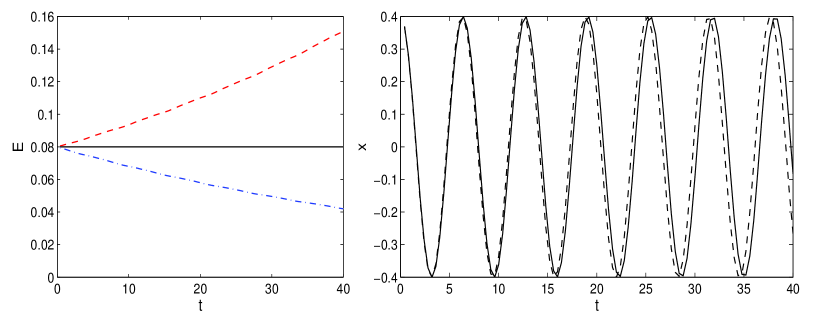
Figure 1: Results of the epicycle test, using $\Omega=1$, $q=3/2$, and one test particle with initial amplitude $A=0.4$, at fixed time step $h=0.4$. Left: Total energy of the test particle integrated using explicit (dashed), semi-implicit (solid) and fully-implicit (dash-dotted) methods. Right: Particle radial orbit integrated using the semi-implicit method (solid) compared with analytical solution (dashed).

We integrate a test particle and follow its epicyclic orbit using different particle integrators and examine the particle trajectory and energy conservation. In particular, we consider three 2nd order integrators, namely, the semi-implicit and fully-implicit integrators introduced in §3, and we add an explicit integrator based on the modified Euler method for comparison purpose. In Figure 1, we see that the semi-implicit method conserves total energy exactly. The particle orbit is closed, and the truncation error exhibits as a phase shift relative to the analytical solution. The phase error diminishes as $h^{2}$ (not shown in the figure), as expected. Note that in order to make the errors significant, we have chosen a rather large time step $h=0.4\Omega^{-1}$. In typical numerical simulations, the time step and thus phase error is much smaller. From Figure 1, we also see that the test particle gains energy and drifts away from the guiding center when using the explicit method, while it loses energy and gyrates into the guiding center when using the fully-implicit method. This result is quite general.

This test demonstrates that the semi-implicit method preserves the geometric properties of particle orbits, and moreover, it is efficient because it evaluates the drag force (therefore interpolation) only once per step. Therefore, in most applications we prefer to use this integrator.

4.2 Particle-Gas Deceleration Test

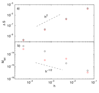
Figure 2: Error in position (a) and total momentum density (b) as a function of time step length $h$ in the particle-gas deceleration test. We choose the particle to gas mass ratio to be 1, and the initial velocities of particles and gas are both 1, but in opposite directions. The particle stopping time is set to $t_{\rm stop}=2$. Errors are measured at $t=1$. Red squares: semi-implicit integrator; Black circles: fully-implicit integrator.

In the second problem, we consider the motion of a collection of particles in a uniform gas. The spatial distribution of the particles is uniform. Gas drag and feedback are included in the test. We work in the frame where the total momentum in particles and gas is zero. Let ${\boldsymbol{w}}_{0}$ be the particle initial velocity, then all the particles evolve as

$$S(t)=\frac{w_{0}t_{\rm stop}}{1+\epsilon}[1-e^{-(1+\epsilon)t/t_{\rm stop}}]\ ,$$ (23)

where $\epsilon$ is the overall particle to gas mass ratio, and $S$ is the distance a particle has traveled.

In our first test, we choose $\epsilon=1,t_{\rm stop}=2,w_{0}=1$, and gas with density $\rho_{g}=1$. We evolve the system to $t_{e}=1$ with constant time step $h$ using the semi-implicit and the fully-implicit integrators. In Figure 2a we plot the position error $\Delta S$ at $t_{e}=1$ as a function of $h$. It is clear that the cumulative position error scales with $h^{2}$, indicating that our particle-gas hybrid code has achieved second order accuracy. Figure 2b shows the total momentum density at $t_{e}=1$ as a function of $h$. We see that our hybrid scheme conserves linear momentum within machine accuracy (to the level of $10^{-16}$). The total momentum at $t_{e}=1$ increases with decreasing $h$, which reflects the accumulation of round-off error with increasing number of time steps. For uncorrelated round-off errors, one would expect $h^{-1/2}$ scaling. The slightly steeper slope reflects a certain level of correlation in the round-off errors.

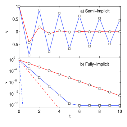
Figure 3: Numerical evolution of particle velocity in the stiff regime of the particle-gas deceleration test. The time step is fixed to $h=1$. Panels (a) and (b) show the results from the semi-implicit integrator and fully-implicit integrator respectively. Black circles connected by red solid lines: $t_{\rm stop}=0.2$. Black squares connected by blue solid lines: $t_{\rm stop}=0.02$. In panel (b), we further show expected evolution of velocity in the two cases: Red dashed line for $t_{\rm stop}=0.2$ and blue dash-dotted line for $t_{\rm stop}=0.02$. Note that in panel (a) we use a linear scale while in panel (b) we use a log scale.

Next we test the integrators in the stiff regime. To do so, we fix the time step $h=1$, and choose $t_{\rm stop}$ to be less than $h$. The other parameters are the same as in the previous test ($\epsilon=1,w_{0}=1$). We evolve the system to $t_{e}=10$, using $t_{\rm stop}=0.2$ and $t_{\rm stop}=0.02$. In Figure 3 we show the time evolution of particle velocity from the semi-implicit and the fully-implicit integrators. We see that with the fully-implicit integrator, the particle velocity (thus the gas velocity, due to momentum conservation) rapidly drops to zero, and smaller $t_{\rm stop}$ leads to faster damping [actually $v^{(n+1)}\sim 2(t_{\rm stop}/h)^{2}v^{(n)}$]. Because $t_{\rm stop}$ is not resolved, the damping rate is slower than theoretical values, but still is rapid as relative velocity $v$ drops several orders of magnitude in each time step. With the semi-implicit integrator, however, the particle velocity undergoes damped oscillation. The smaller $t_{\rm stop}$ is, the slower the particle velocity damps [actually $v^{(n+1)}\sim-(1-4t_{\rm stop}/h)v^{(n)}$], opposite to the trend found in the fully-implicit integrator. In the limit $t_{\rm stop}=0$, the particle velocity never dies away. The behavior of the semi-implicit integrator in this regime exactly resembles a damped harmonic oscillator, which makes it difficult for particles to get rid of extra relative velocity with respect to gas. This situation is problematic because if the gas itself undergoes some other oscillation with a similar frequency, the amplitude of the oscillator may be quickly amplified rather than damped due to (numerical) resonant interactions. Therefore, for stability considerations, we use the fully-implicit integrator when $t_{\rm stop}\lesssim h$.

4.3 Streaming Instability in the Linear Regime

The most stringent test of our code is the streaming instability linear growth rate test using eigenmodes provided by YJ07. These eigenmodes are built from the Nakagawa-Sekiya-Hayashi (NSH) equilibrium [Nakagawa et al., 1986; also see equation (7) of YJ07]. The NSH equilibrium refers to the equilibrium between solids and gas in unstratified Keplerian disks, in which gas is partially supported by a radial pressure gradient. Establishing the NSH equilibrium numerically requires exact balance among all force terms. With the help of the particle advection scheme as well as careful treatment of predictor and corrector step momentum feedback (see §2 and §3 for details), we are able to establish the exact NSH equilibrium in our code (i.e., net force on both the gas and particles is zero to machine precision). The eigenmodes of the streaming instability are characterized by dimensionless wave numbers $K_{x}\equiv k_{x}\eta v_{k}/\Omega$ and $K_{z}\equiv k_{z}\eta v_{k}/\Omega$. Taking $\eta v_{k}=0.05c_{s}$ and setting the box size to be one wavelength, we have $K_{x}=0.05(c_{s}/\Omega)(2\pi/L_{x})$, and similarly in the $z$ direction. We fix the box size to be $L_{x}=L_{z}=2$, therefore, $K_{x}$ (and $K_{z}$) sets the sound speed. We construct eigenvectors of density and velocity perturbations using formula (10) and Table 1 in YJ07. We use one particle per cell and each particle is located at cell center initially. In order to generate particle density profile of $\rho_{d}=1+A\cos{k_{x}x}\cos{k_{z}z}$ (we take $A=10^{-6}$), we shift particle positions in the radial ($x$) direction, with the amount of shift proportional to $\cos{k_{z}z}$.

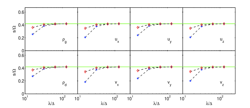
(a) Test “linA”

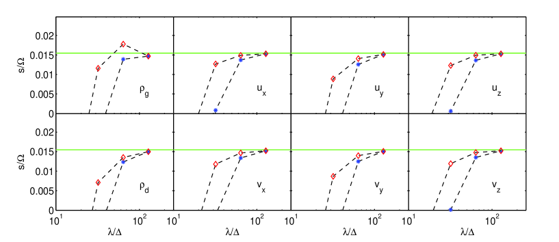
(b) Test “linB”

Figure 4: Measured growth rate of the streaming instability eigenmodes “linA” (a) and “linB” (b) adopted from Youdin & Johansen (2007) using the semi-implicit integrator. Solid line marks the theoretical growth rate, and dashed lines with symbols label the measured growth rate as a function of grid resolution (number of cells per wavelength). Asterisks correspond to evolution using fixed CFL number 0.8, diamonds correspond to fixed time step (set by CFL=0.8 with 128 cells).

The test suite in YJ07 aims at measuring the numerical growth rate of the streaming instability eigenmodes as a function of grid resolution. It consists of two problems, both using $\tau_{s}=0.1$ particles. The test “linA” has particle to gas mass ratio $\epsilon=3$ and $K_{x}=K_{z}=30$. The predicted growth rate is $s=0.4190204\Omega$. The second test “linB” has $\epsilon=0.2$ and $K_{x}=K_{z}=6$. This test is more challenging because the mode grows very slowly, with $s=0.015476\Omega$. We consider grid resolutions of 16, 32, 64 and 128 cells per wave length. Figure 4 shows our test results using the semi-implicit integrator. In each test, we conduct two set of runs, one with fixed Courant-Friedrichs-Lewy number CFL=0.8, and the other with a fixed time step (or CFL=0.1, 0.2, 0.4, 0.8 for each resolution). For reference, the time step with lowest resolution (16 cells per wavelength) and CFL=0.8 is $\Omega h=2.6\times 10^{-4}$ for “linA” and $\Omega h=1.3\times 10^{-3}$ for “linB”. Both semi-implicit and fully-implicit methods are considered, and the results are almost identical (since the time step is much smaller than $t_{\rm stop}$). We see that our code converges very well to the predicted growth rate in the run “linA”. Small time step helps with convergence. For the more challenging ‘linB” test, we get slower convergence. In particular, the mode does not grow for 32-cell resolution using CFL=0.8. Better temporal resolution again improves the performance.

These test results show that with CFL=0.8, about 64 cells are needed to see growth (e.g., test linB), although 16 cells seem to be sufficient to capture the most unstable modes (e.g., test linA). Viewed from the results, our measured linear growth rates are similar to (and even closer to semi-analytic values than) those of Balsara et al. (2009) and Miniati (2010), who employ similar MHD code but different hybrid schemes. Our method is less accurate than that presented in YJ07, which is not surprising given the fact that our code is second order accurate (both spatial and temporal) while the Pencil code used by YJ07 is sixth order spatial and third order temporal accurate for smooth flows, such as in this test.

The test problems “linA” and “linB” provided in YJ07 both adopt relatively large particle stopping time $\tau_{s}=0.1$. Since we will perform SI simulations on a size distribution of particles with stopping time down to $10^{-3}$, additional code test is needed to justify the ability of our code. In Appendix A, we provide two more linear growth tests for particles with $\tau_{s}=10^{-2}$ and $\tau_{s}=10^{-3}$. Numerical convergence to the analytical growth rate is again achieved, although slightly higher resolution is required to reach the convergence.

5 Convergence of Streaming Instability

As an application of our hybrid code, we study the streaming instability in the non-linear regime. Such calculations have been performed and comprehensively analyzed by JY07. In this paper, we focus on the numerical convergence of physical properties in the saturated state, which was not fully explored in JY07. Understanding the convergence properties of hydrodynamic simulations of the streaming instabilities is important before adding more complicated physics (such as MHD), and interpreting the reliability of such simulations.

We study the numerical convergence using 2D simulations in the $x-z$ (radial-vertical) plane in which both the grid resolution and the number of (super-) particles vary. By using 2D simulations, we can explore a wide range of resolutions that is not possible in fully 3D simulations. Moreover, the results of 2D and 3D simulations are similar (JY07), thus one expects the numerical convergence properties of 2D simulations are similar to those in 3D as well.

The two most significant effects of the streaming instability are the concentration of particles into dense clumps, and the generation of turbulence and/or waves. The former can be characterized by the probability distribution function (PDF) of particle densities, while the latter can be characterized by the turbulent velocity, diffusion coefficient and momentum flux. We investigate the numerical convergence of these two aspects in §5.2 and §5.3 respectively.

5.1 Simulation Setup

We perform simulations of the streaming instability using an isothermal equation of state and neglecting vertical gravity. In this case, the properties of the streaming instability is largely determined by two parameters, the particle stopping time $\tau_{s}$ and the overall mass ratio between particles and gas $\epsilon$. The drift velocity $\eta v_{K}$ does not serve as an independent variable, but it sets the length scale of the problem, that is, all length scales can be measured in units of $\eta r\equiv\eta v_{K}/\Omega$. The isothermal sound speed $c_{s}$ is also a model parameter, but it is much less important because the gas motion is almost incompressible (Youdin & Goodman, 2005, JY07). We adopt $\eta v_{K}/c_{s}=0.05$ throughout this paper, which roughly matches the value expected at 1AU in the MMSN model.

As shown by JY07, there are two basic “modes” to the non-linear saturation of the streaming instability. For marginally coupled and larger particles ($\tau_{s}\gtrsim 1$), the instability develops for a wide range of $\epsilon$, around 1. In the saturated state, particles concentrate into long stripes, which are mostly aligned with the vertical direction and are slightly tilted in the radial direction. For tightly coupled particles ($\tau_{s}\ll 1$), prominent instability develops only when $\epsilon\gtrsim 1$, and the turbulent state consists of large voids with narrow particle streams. The turbulence is much weaker than the previous case (see Figure 2 and Figure 5 of JY07 for each of the two “modes”, also see our Figure 5 below). We have also performed a series of simulations with a wide range of parameters ($\tau_{s}$ and $\epsilon$), and have reproduced all the results in JY07. We use the semi-implicit integrator in all the tests in this section, and results from the other two integrators are similar, since the time step is at least 10 times smaller than $t_{\rm stop}$ in all test runs.

To study convergence, we choose two test problems that are representative of the two saturation “modes” described by JY07 . The first problem is the same as their run AB. The run parameters include: $\tau_{s}=0.1$, $\epsilon=1.0$, $L_{x}=L_{z}=2\eta r$. The second problem uses parameters from their run BA, with $\tau_{s}=1.0$, $\epsilon=0.2$, $L_{x}=L_{z}=40\eta r$. We choose the “standard” grid resolution to be $256^{2}$, and $N_{\rm pc}=9$ particles per grid cell. The typical time step is given by $h\sim{\rm CFL}(L_{x}/N)/c_{s}$ where $N$ is the number of grid cells in one direction. For the standard grid resolution and ${\rm CFL}=0.8$, we have $\Omega h\approx 3\times 10^{-4}$ for run AB, and $\Omega h\approx 6\times 10^{-3}$ for run BA. We then conduct a series of runs for each problem. First, we change the grid resolution from $64^{2}$ to $2048^{2}$, with the number of particles per cell fixed at 9. Note that increasing spatial resolution at fixed ${\rm CFL}$ number is accompanied by the increase of temporal resolution, which is also important for driving to convergence, as we discussed in §4.3. Secondly, we fix the grid resolution to be $256^{2}$, and change the number of particles per cell, $N_{\rm pc}=1,4,9,16$ and $25$. In each of these runs, particles are initialized with random positions within the simulation box, with velocities taken from the NSH equilibrium. All these runs are tabulated in the first three columns of Table 1, where each variation of the AB or BA runs is assigned with a run number. Our fiducial runs are AB3 and BA3, while our runs AB9 and BA9 have exactly the same numerical parameters as that in JY07.

The AB runs are fully saturated after about $16\Omega^{-1}$ and the BA runs do not saturate until about $160\Omega^{-1}$. We choose the saturation time for the two runs to be some later time $T_{s}^{(AB)}=30\Omega^{-1}$, $T_{s}^{(BA)}=300\Omega^{-1}$, after which we start collecting data from the simulations and perform measurements. In Figure 5, we show images of the particle density with different grid resolution ($64^{2}$, $256^{2}$, $1024^{2}$ from top to bottom) for runs AB (left) and BA (right) at saturation ($t=T_{s}$). Our standard runs (middle panels) resemble the last panels of Figure 4 and Figure 5 in JY07. For the BA run series, we see that the bulk patterns of particle density do not vary much with grid resolution, although more and more detailed features are revealed in the higher resolution simulations. For the AB run series, all three grid resolutions show cavitation and particle streams as described in JY07, however, the scale of particle clumping becomes smaller as one uses finer resolutions. A resolution of $256^{2}$ appears to be necessary to capture the prominent features in the particle density pattern. The results of these runs will serve as the starting point of our more quantitative study of numerical convergence in the next two subsections, using physical quantities averaged over the period between $T_{s}$ and $T_{e}$, where $T_{e}^{(AB)}=80\Omega^{-1}$ for AB runs and $T_{e}^{(BA)}=1500\Omega^{-1}$ for BA runs.

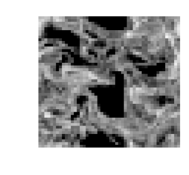
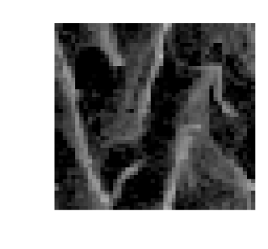
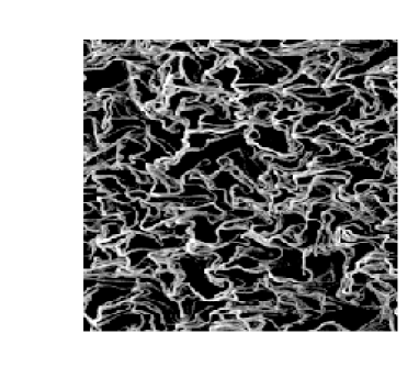
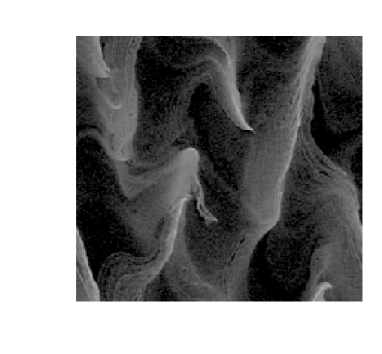
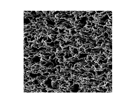
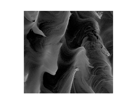
Figure 5: Snapshots of particle densities in the $x-z$ plane of run AB (left) and BA (right) at saturation of the streaming instability $T=T_{s}$ with different grid resolutions: $64^{2}$ (top), $256^{2}$ (middle) and $1024^{2}$ (bottom). All simulations use $9$ particles per cell. Particle densities are shown with log scale, ranging between $0.1$ to $10$ of the gas density for the AB runs, and between $0.01$ to $100$ for the BA runs. White regions indicate high density. The size of the box is $L_{x}=L_{z}=2\eta r$ for run AB, and $L_{x}=L_{z}=40\eta r$ for run BA.

5.2 Particle Concentration

Probably the most important property of the streaming instability is its ability to concentrate particles. In JY07, it was shown that the maximum particle density resulting from the streaming instability can reach as high as $10^{3}$ times background particle density. Such high densities are sufficient to make the clumps gravitationally bound, promoting the formation of planetesimals in PPDs (Johansen et al., 2007). The concentration of particles is best demonstrated by the cumulative probability distribution function (PDF) of particle densities. It measures the fraction of particles whose ambient particle density exceeds a given value. In Figure 6 we show the particle density distribution from the series of AB and BA runs. Note that in the horizontal axis, we have normalized particle density to the averaged particle density in the simulation box.

The ability for our code to handle the particle clump is reflected in the stiffness parameter $\chi$ defined in equation (11). We have tested that the maximum value of $\chi$ in our AB runs is about $\chi_{\rm max}\sim 0.2$ in $64^{2}$ resolution, and it monotonically drops to $\chi_{\rm max}\sim 0.004$ in $2048^{2}$ resolution. For the BA runs, $\chi_{\rm max}$ stays less than $0.5$ for most of the time and for all resolutions, but reaches as large as $2.0$ in a few transients in the highest resolution run. The duration of the transients is so short that their contribution to the PDF is far below $10^{-5}$ and is not visible in our Figure 6. These facts show that the particle clumps are properly handled in our code and the obtained PDFs are not affected by the possible stiffness in the dense clumps.

Our results agree quantitatively with Figure 11 of JY07 (our AB9 and BA9 $256^{2}$ runs resolution with $N_{\rm pc}=25$). The PDFs calculated from our AB runs are very robust, in the sense that using longer period of averaging or using different initial random seeds do not produce any visible changes in the plot. For the BA runs, there can be some uncertainties in the calculation of the PDFs, mostly because that there are only a few dense clumps in the simulation box, the long term stochastic evolution of these big clumps makes the calculated PDFs more or less dependent on the period of time averaging. Nevertheless, we have averaged the PDFs over as long as nearly 200 orbits, which is about 170 times the correlation time of the clumps (which is about $7\Omega^{-1}$, see Figure 13 of JY07), such uncertainty is expected to be small and does not affect the main features to be discussed below.

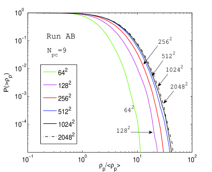
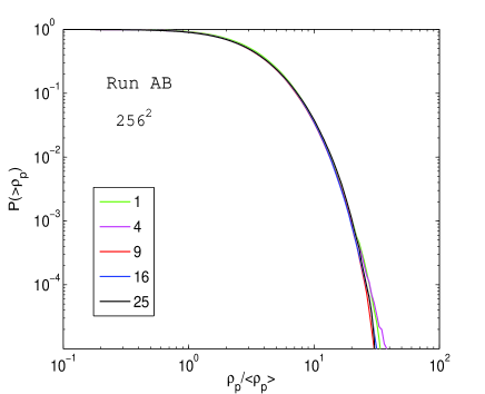
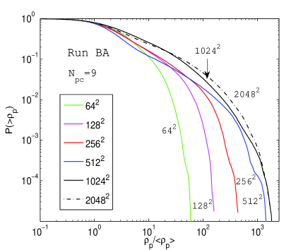
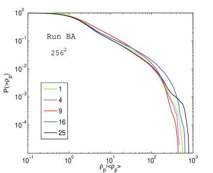
Figure 6: The cumulative probability distribution function of particle density. Top and bottom panels show results from the AB and BA runs respectively. On the left panels, number of particles per cell $N_{\rm pc}$ is fixed to 9. Green, magenta, red, blue and black curves label results from $64^{2}$, $128^{2}$, $256^{2}$, $512^{2}$ and $1024^{2}$ grid resolutions respectively. The dash-dotted curve shows the results from $2048^{2}$ resolution run for comparison. On the right panels, grid resolution is fixed to be $256^{2}$, while $N_{\rm pc}$ varies to be $1$, $4$, $9$, $16$ and $25$, as labeled by green, magenta, red, blue and black curves.

The left panels of Figure 6 show the effect of grid resolution on the density PDFs: higher grid resolution leads to stronger particle clumping. Both the maximum particle density is higher, and the number of particles residing in dense clumps is larger at higher resolutions. For the AB runs, the PDFs from the $512^{2}$ resolution run is almost identical to higher resolution runs, indicating convergence. For the BA runs, the small number of dense clumps in the simulation box makes convergence more difficult by averaging over a finite time period. Nevertheless, viewing from the PDF curves, it appears that convergence is finally reached at $1024^{2}$ resolution.

We have also studied the numerical convergence with number of particles in the simulation box. On the right panels of Figure 6, we see that for both runs AB and BA, the PDFs depend very weakly on $N_{\rm pc}$. In the AB runs, the five curves almost overlap with each other. In BA runs, however, there is larger scatter. Again, such scatter is most likely due to the small number of clumps. In fact, we have compared the BA run PDFs between short ($T_{e}-T_{s}=500\Omega^{-1}$) and long ($T_{e}-T_{s}=1200\Omega^{-1}$, shown in the figure) averaging period. The PDFs from longer averaging converges show better convergence. We expect the scatter to become smaller if we run BA series for much longer time. In all, we conclude that one can use as small as only one particle per cell to accurately capture the density distributions of the solids.

5.3 Turbulence Properties

The streaming instability generates turbulence which differs significantly from the laminar state described by the NSH equilibrium. The turbulence is accompanied by particle concentration, as discussed in the previous subsection. Understanding the turbulent state is important since it may strongly affect the settling process as well as the radial transport of solids in the PPDs (JY07, Bai & Stone, 2010a). Similar to JY07, we have computed a number of physical quantities to characterize the turbulence properties generated from the streaming instability, including: 1) The turbulent Mach number ($Ma$) in three directions, calculated from the root mean square of gas velocity fluctuations; 2) Mean radial drift velocity of the particles, normalized by the NSH radial drift velocity $\overline{v_{x}}/\overline{v_{x}}^{NSH}$; 3) Turbulent diffusion coefficient for particles $D$, calculated using the method outlined in §5.3 of JY07; and 4) The time and spatial averaged Reynolds stress ${\mathcal{F}}\equiv\rho_{g}u_{x}(u_{y}-v_{K})$, divided by the Reynolds stress in the NSH equilibrium (note the quantity we measure is different from ${\mathcal{F}}_{\mathcal{L},x}$ in JY07). Properties (1), (2) and (4) are calculated directly from spatial and time averaging from the entire simulation box. The $1\sigma$ uncertainties are estimated from the standard deviation in the time sequence. In the calculation of the diffusion coefficient, we measure the standard deviation of the distance traveled by tracer particles at different time intervals $\sigma_{x}(\Delta t),\sigma_{z}(\Delta t)$. We then fit the diffusion coefficient using $\sigma^{2}_{x,z}(\Delta t)=2D_{x,z}\Delta t$. The maximum $\Delta t$ has been chosen to be $32\Omega^{-1}$ for AB runs, $320\Omega^{-1}$ for BA runs. The uncertainty of the diffusion coefficient is directly given by the linear regression estimate. The results are summarized in Table 1.

From Table 1 we see that the gas flow properties, namely the turbulent Mach number and the Reynolds stress, depend relatively weakly on the grid resolution and number of particles in the simulation box. This trend is also true for the radial drift velocity of the particles. In the AB series of runs, all these quantities agree with each other once the grid resolution reaches $256^{2}$. Smaller resolution runs produce somewhat different values, but with larger fluctuations. Note that in Figure 5, the typical size of particle stripes from the $1024^{2}$ run (AB5) is apparently smaller than that from the $256^{2}$ run (AB3). However, the statistical properties of gas flow from these two runs are indistinguishable. In this sense, $256^{2}$ resolution is sufficient to capture the essential turbulent properties for the AB runs. For BA run series, the measurements from even the lowest resolution run $64^{2}$ agree very well with other higher resolution runs. Such numerical convergence behavior is very different from the convergence of particle concentration properties discussed in §5.2.

The measurements of the diffusion coefficient in the radial and vertical directions, however, show larger variations among different runs for both AB and BA series. Such variations show up not only between different grid resolutions, but also at fixed resolution, varying the number of particles in the simulation box also makes a difference. The differences even exceed the $1\sigma$ uncertainties in a number of cases. Moreover, there is no systematic trend on such variances, especially in the BA run series. In the AB runs, it appears that towards higher resolution, the diffusion coefficient becomes smaller. Given the fact that bulk flow properties converge well at modest resolutions, the variation of diffusion coefficient measured from different runs, especially those with grid resolution no less than $256^{2}$, may be taken as uncertainties from the numerical simulations. The uncertainties in the measured diffusion coefficient would be about 20%, for both AB and BA runs.

Table 1: Turbulence Properties.

Run	Resolution	$N_{\rm pc}$	$Ma_{x}\ ^{1}$	$Ma_{y}\ ^{1}$	$Ma_{z}\ ^{1}$	$\overline{v_{x}}/\overline{v_{x}}^{NSH}\ {}^{2}$	$D_{x}\ ^{3}$	$D_{z}\ ^{3}$	${\mathcal{F}}_{\rm Re}/{\mathcal{F}}^{\rm NSH}_{\rm Re}\ {}^{4}$
AB1	$64^{2}$	9	$0.97(15)\times 10^{-2}$	$2.44(15)\times 10^{-2}$	$0.81(15)\times 10^{-2}$	1.40(80)	$2.64(08)\times 10^{-5}$	$7.01(29)\times 10^{-5}$	1.72(79)
AB2	$128^{2}$	9	$1.23(07)\times 10^{-2}$	$2.45(07)\times 10^{-2}$	$0.98(07)\times 10^{-2}$	1.88(27)	$4.61(05)\times 10^{-5}$	$9.50(63)\times 10^{-5}$	2.38(30)
AB3	$256^{2}$	9	$1.24(04)\times 10^{-2}$	$2.47(04)\times 10^{-2}$	$0.78(04)\times 10^{-2}$	2.14(07)	$5.12(04)\times 10^{-5}$	$3.01(06)\times 10^{-5}$	2.67(12)
AB4	$512^{2}$	9	$1.25(03)\times 10^{-2}$	$2.47(03)\times 10^{-2}$	$0.78(03)\times 10^{-2}$	2.21(06)	$4.58(04)\times 10^{-5}$	$2.89(07)\times 10^{-5}$	2.69(10)
AB5	$1024^{2}$	9	$1.24(03)\times 10^{-2}$	$2.47(03)\times 10^{-2}$	$0.76(03)\times 10^{-2}$	2.22(05)	$4.37(06)\times 10^{-5}$	$2.28(02)\times 10^{-5}$	2.68(09)
AB6	$256^{2}$	1	$1.23(05)\times 10^{-2}$	$2.46(05)\times 10^{-2}$	$0.76(05)\times 10^{-2}$	2.13(08)	$5.11(06)\times 10^{-5}$	$2.76(07)\times 10^{-5}$	2.67(16)
AB7	$256^{2}$	4	$1.24(05)\times 10^{-2}$	$2.46(05)\times 10^{-2}$	$0.80(05)\times 10^{-2}$	2.13(08)	$5.16(03)\times 10^{-5}$	$3.15(10)\times 10^{-5}$	2.67(15)
AB3	$256^{2}$	9	$1.24(04)\times 10^{-2}$	$2.47(04)\times 10^{-2}$	$0.78(04)\times 10^{-2}$	2.14(07)	$5.12(04)\times 10^{-5}$	$3.01(06)\times 10^{-5}$	2.67(12)
AB8	$256^{2}$	16	$1.26(06)\times 10^{-2}$	$2.47(06)\times 10^{-2}$	$0.81(06)\times 10^{-2}$	2.16(09)	$5.14(04)\times 10^{-5}$	$3.29(07)\times 10^{-5}$	2.71(16)
AB9	$256^{2}$	25	$1.26(05)\times 10^{-2}$	$2.46(05)\times 10^{-2}$	$0.83(05)\times 10^{-2}$	2.15(08)	$5.38(05)\times 10^{-5}$	$3.25(08)\times 10^{-5}$	2.72(16)
BA1	$64^{2}$	9	$1.19(08)\times 10^{-2}$	$1.84(08)\times 10^{-2}$	$3.88(08)\times 10^{-2}$	0.65(07)	$2.18(06)\times 10^{-3}$	$1.01(04)\times 10^{-2}$	0.59(07)
BA2	$128^{2}$	9	$1.20(10)\times 10^{-2}$	$1.87(10)\times 10^{-2}$	$4.03(10)\times 10^{-2}$	0.65(06)	$2.36(06)\times 10^{-3}$	$1.37(06)\times 10^{-2}$	0.61(06)
BA3	$256^{2}$	9	$1.21(11)\times 10^{-2}$	$1.81(11)\times 10^{-2}$	$3.88(11)\times 10^{-2}$	0.66(07)	$2.30(09)\times 10^{-3}$	$0.97(05)\times 10^{-2}$	0.62(08)
BA4	$512^{2}$	9	$1.16(11)\times 10^{-2}$	$1.83(11)\times 10^{-2}$	$3.93(11)\times 10^{-2}$	0.70(06)	$2.29(11)\times 10^{-3}$	$1.39(05)\times 10^{-2}$	0.67(06)
BA5	$1024^{2}$	9	$1.36(09)\times 10^{-2}$	$1.88(09)\times 10^{-2}$	$3.89(09)\times 10^{-2}$	0.60(06)	$2.20(05)\times 10^{-3}$	$1.16(08)\times 10^{-2}$	0.56(06)
BA6	$256^{2}$	1	$1.17(12)\times 10^{-2}$	$1.86(12)\times 10^{-2}$	$4.00(12)\times 10^{-2}$	0.67(08)	$2.71(11)\times 10^{-3}$	$1.44(05)\times 10^{-2}$	0.64(08)
BA7	$256^{2}$	4	$1.12(05)\times 10^{-2}$	$1.80(05)\times 10^{-2}$	$3.92(05)\times 10^{-2}$	0.71(04)	$1.87(03)\times 10^{-3}$	$1.23(05)\times 10^{-2}$	0.68(04)
BA3	$256^{2}$	9	$1.21(11)\times 10^{-2}$	$1.81(11)\times 10^{-2}$	$3.88(11)\times 10^{-2}$	0.66(07)	$2.30(09)\times 10^{-3}$	$0.97(05)\times 10^{-2}$	0.62(08)
BA8	$256^{2}$	16	$1.16(10)\times 10^{-2}$	$1.83(10)\times 10^{-2}$	$4.00(10)\times 10^{-2}$	0.69(05)	$2.15(06)\times 10^{-3}$	$1.35(06)\times 10^{-2}$	0.66(05)
BA9	$256^{2}$	25	$1.14(08)\times 10^{-2}$	$1.81(08)\times 10^{-2}$	$3.89(08)\times 10^{-2}$	0.70(06)	$2.23(08)\times 10^{-3}$	$1.32(05)\times 10^{-2}$	0.67(06)

The number in parenthesis quotes the $1\sigma$ uncertainty of the last two digits. See §5.3 for details.

¹ Mach number in the radial, azimuthal and vertical directions.

² Radial drift velocity of particles, normalized by the NSH value.

³ Turbulent diffusion coefficient of the particles in the radial and vertical directions.

⁴ Mean Reynolds stress of the gas, normalized by the NSH value.

6 Summary and Conclusion

We have presented the implementation of a hybrid particle-gas scheme in the grid-based Athena MHD code. The particle and gas are assumed to be coupled aerodynamically, and a size distribution of particle species with different stopping times is allowed. Our implementation is extendable to include gravitational coupling, which is left for future work. The main purpose for the code development is to study the dynamics of gas and solids in protoplanetary disks (PPDs). The solid size range where the aerodynamic coupling has significant effects in PPDs roughly spans from millimeter to a few tens or hundreds meter sized bodies, depending on the disk model and location, and this is the regime most relevant for studying planetesimal formation (Chiang & Youdin, 2009). In this paper we mainly address the numerical method and code performance. In a forthcoming paper (Bai & Stone, 2010a), we will describe applications to PPDs.

The numerical algorithm of our hybrid code is based on a second-order accurate predictor-corrector scheme. The algorithm is different from other existing codes (YJ07,Balsara et al., 2009; Miniati, 2010), and is very simple and robust. Our implementation of particle-gas coupling is fully conservative: backreaction from the particles to the gas is treated carefully that the total momentum is conserved exactly. Our hybrid code works well in non-stiff regime of particle-gas coupling, as well as the stiff regime without significant particle mass loading [i.e., the parameter $\chi$ defined in equation (11) does not exceed order unity]. This is made possible by two implicit particle integrators. These include a semi-implicit integrator, generalized from the second order leap-frog integrator, which has much better stability properties than any explicit methods, and which preserves the geometric properties of particle orbit exactly in the limit of zero drag force. In addition, a fully-implicit integrator is designed for treating extremely stiff problem when particle stopping time is much smaller than the simulation time step. We have extensively tested our code performance, including the linear growth rate test of the streaming instability. Subsequent test on the non-linear saturation of the streaming instability further confirms that our code performs as good as the higher order finite difference Pencil code, as the flow properties measured from our simulations agree well with the results by JY07.

We have also studied the numerical convergence of our method in the non-linear regime of the streaming instability. We pick two representative runs from JY07 and have performed a series of simulations by varying grid resolutions and total number of particles in the simulation box. We find that the convergence properties in the non-linear regime is very different and more complicated than those in the linear regime. The main conclusions drawn from this convergence study are summarized below.

1. Requirement for numerical convergence strongly depends on particle stopping time $\tau_{s}$. For $\tau_{s}=0.1$, about $128$ cells per $\eta r$ is necessary for convergence.

2. Equal number of particles and grid cells is sufficient for numerical convergence.

3. Gas flow properties converge very well at modest grid resolution and is not sensitive to number of particles used in the simulation.

4. Particle concentration properties converge at very high grid resolution. Higher resolution leads to stronger clumping.

5. Particle diffusion properties depend on the numerical setup in a subtle way, leading to about $\pm 20\%$ uncertainties in the measurements.

These convergence tests provide useful information on the reliability and uncertainty of this kind of hybrid simulations of the particle-gas interaction. They also provide a guide on the choice of grid resolution and number of particles for future simulations of similar and more complicated problems. Although all the results are based on vertically unstratified simulations, we may generalize these criteria to simulations with vertical gravity. Also, with more than one particle species, we expect numerical convergence with one particle per cell per particle species, where different particle species have different stopping times.

Recently, Rein et al. (2010) addressed the validity of the super-particle approximation in numerical simulations with particles. They emphasized that it is essential to maintain the important timescales in the scaled system (i.e. the simulation) to be equivalent to the timescales in the real system, otherwise one cannot achieve numerical convergence. This is unlikely to be relevant to the problem considered in this paper because we have not added gravitational interaction nor particle collisions. The only time scales to be fixed are the orbital period and the stopping time, which are combined into the dimensionless stopping time $\tau_{s}$. Our results imply that numerical convergence can still be achieved when aerodynamic interaction between particle and gas is added, strengthen conclusions of Rein et al.

Appendix A Additional Linear Growth Rate Test of the Streaming Instability

The linear and non-linear SI simulations in this paper adopt relatively large particle stopping times $\tau_{s}\leq 0.1$. In this appendix we provide two additional linear growth test problems to test code performance for smaller $\tau_{s}$. The simulation set up is described section 4.3, the first test (“linC”), $\tau_{s}=0.01$, $\epsilon=2$, $K_{x}=K_{z}=1500$, the analytical growth rate is $s=0.5981$. In the second test (“linD”), $\tau_{s}=10^{-3}$, $\epsilon=2$, and $K_{x}=K_{z}=2000$, with growth rate $s=0.3154$. Both modes are chosen to be close to the fastest growth mode. However, these tests are more computationally costly because of the larger $K$. The eigenvectors of the two modes are listed in Table 2. The table format is the same as Table 1 of YJ07.

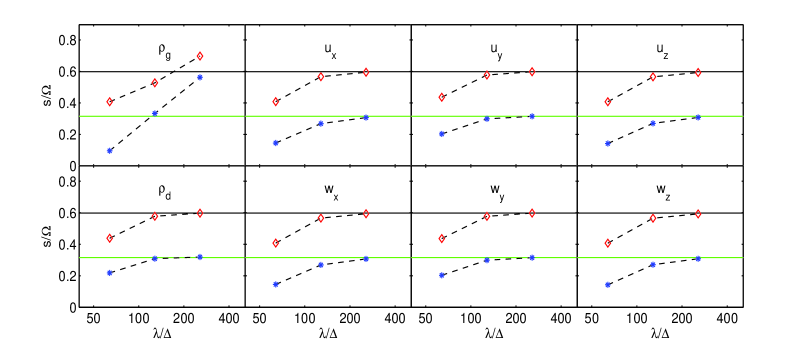
Figure 7: Measured growth rate of the streaming instability eigenmodes “linC” (diamonds) and “linD” (asterisks) using the semi-implicit integrator. Solid line marks the theoretical growth rate, and dashed lines with symbols label the measured growth rate as a function of grid resolution (number of cells per wavelength). We use CFL$=0.4$ in all the tests.

In Figure 7 we show the numerical growth rate measured as a function of grid resolution for the two tests “linC” and “linD”. The CFL number is fixed at 0.4 for these tests. Note that for smaller $\tau_{s}$, the perturbations on the gas is extremely small, and capturing the correct growth rate on the gas is very difficult. For other quantities, numerical convergence to theoretical growth rate is clearly reached as shown in the figure, however, for smaller $\tau_{s}$, higher resolution of about $128$ cells per wavelength is needed for numerical convergence.

Table 2: Test Mode Eigensystems.

Test	${\widetilde{u}}_{x}$	${\widetilde{u}}_{y}$	${\widetilde{u}}_{z}$	${\widetilde{\rho}}_{g}$	${\widetilde{w}}_{x}$	${\widetilde{w}}_{y}$	${\widetilde{w}}_{z}$	$\omega$
linC $\tau_{s}=10^{-2},\ \epsilon=2$	$-0.1598751$	$0.1164423$	$0.1598751$	$8.684872$e-8	$-0.1567174$	$0.1159782$	$0.1590095$	$0.1049236$
($K_{x}=K_{z}=1500$)	$+0.0079669i$	$+0.0122377i$	$-0.0079669i$	$+5.350037$e-7$i$	$+0.0028837i$	$+0.0161145i$	$-0.0024850i$	$+0.5980690i$
linD $\tau_{s}=10^{-3},\ \epsilon=2$	$-0.1719650$	$0.1918893$	$0.1719650$	$2.954631$e-7	$-0.1715840$	$0.1918542$	$0.1719675$	$0.3224884$
($K_{x}=K_{z}=2000$)	$+0.0740712i$	$+0.0786519i$	$-0.0740712i$	$+1.141385$e-7$i$	$+0.0740738i$	$+0.0787371i$	$-0.0739160i$	$+0.3154373i$

Note: the table format is the same as Table 1 of YJ07.

References

- Bai & Stone (2010a) Bai, X.-N. & Stone, J. 2010a, ApJ, accepted, arXiv:1005.4982
- Bai & Stone (2010b) Bai, X.-N. & Stone, J. 2010b, ApJL, submitted, arXiv:1005.4981
- Balsara et al. (2009) Balsara, D. S., Tilley, D. A., Rettig, T., & Brittain, S. D. 2009, MNRAS, 397, 24
- Birdsall & Langdon (2005) Birdsall, C. K. & Langdon, A. B. 2005, Plasma Physics Via Computer Simulation (Taylor & Francis Group, 2005)
- Chiang & Youdin (2009) Chiang, E. & Youdin, A. 2010, Annual Review of Earth and Planetary Sciences, 38, 493
- Cuzzi et al. (1993) Cuzzi, J. N., Dobrovolskis, A. R., & Champney, J. M. 1993, Icarus, 106, 102
- Epstein (1924) Epstein, P. S. 1924, Phys. Rev., 23, 710
- Garaud & Lin (2004) Garaud, P. & Lin, D. N. C. 2004, ApJ, 608, 1050
- Goldreich & Lynden-Bell (1965) Goldreich, P. & Lynden-Bell, D. 1965, MNRAS, 130, 125
- Hawley et al. (1995) Hawley, J. F., Gammie, C. F., & Balbus, S. A. 1995, ApJ, 440, 742
- Hayashi (1981) Hayashi, C. 1981, Progress of Theoretical Physics Supplement, 70, 35
- Johansen & Klahr (2005) Johansen, A. & Klahr, H. 2005, ApJ, 634, 1353
- Johansen et al. (2007) Johansen, A., Oishi, J. S., Low, M.-M. M., Klahr, H., Henning, T., & Youdin, A. 2007, Nature, 448, 1022
- Johansen & Youdin (2007) Johansen, A. & Youdin, A. 2007, ApJ, 662, 627 (JY07)
- Johnson et al. (2008) Johnson, B. M., Guan, X., & Gammie, C. F. 2008, ApJS, 177, 373
- Masset (2000) Masset, F. 2000, A&AS, 141, 165
- Miniati (2010) Miniati, F. 2010, Journal of Computational Physics, 229, 3916
- Morbidelli et al. (2009) Morbidelli, A., Bottke, W. F., Nesvorný, D., & Levison, H. F. 2009, Icarus, 204, 558
- Nakagawa et al. (1986) Nakagawa, Y., Sekiya, M., & Hayashi, C. 1986, Icarus, 67, 375
- Quinn et al. (2009) Quinn, T., Perrine, R. P., Richardson, D. C., & Barnes, R. 2010, AJ, 139, 803
- Rein et al. (2010) Rein, H., Lesur, G., & Leinhardt, Z. M. 2010, A&A, 511, A69
- Shakura & Sunyaev (1973) Shakura, N. I. & Sunyaev, R. A. 1973, A&A, 24, 337
- Stone & Gardiner (2009) Stone, J. M. & Gardiner, T. 2009, New Astronomy, 14, 139
- Stone & Gardiner (2010) Stone, J. M. & Gardiner, T. A. 2010, ApJS, 189, 142
- Stone et al. (2008) Stone, J. M., Gardiner, T. A., Teuben, P., Hawley, J. F., & Simon, J. B. 2008, ApJS, 178, 137
- Weidenschilling (1977) Weidenschilling, S. J. 1977, MNRAS, 180, 57
- Weidenschilling (1980) —. 1980, Icarus, 44, 172
- Youdin & Johansen (2007) Youdin, A. & Johansen, A. 2007, ApJ, 662, 613 (YJ07)
- Youdin & Goodman (2005) Youdin, A. N. & Goodman, J. 2005, ApJ, 620, 459
- Zsom et al. (2010) Zsom, A., Ormel, C. W., Guettler, C., Blum, J., & Dullemond, C. P. 2010, A&A, 513, A57