Criticality of the Mean-Field Spin-Boson Model: Boson State Truncation and Its Scaling Analysis

Abstract

The spin-boson model has nontrivial quantum phase transitions at zero temperature induced by the spin-boson coupling. The bosonic numerical renormalization group (BNRG) study of the critical exponents $\beta$ and $\delta$ of this model is hampered by the effects of boson Hilbert space truncation. Here we analyze the mean-field spin boson model to figure out the scaling behavior of magnetization under the cutoff of boson states $N_{b}$. We find that the truncation is a strong relevant operator with respect to the Gaussian fixed point in $0<s<1/2$ and incurs the deviation of the exponents from the classical values. The magnetization at zero bias near the critical point is described by a generalized homogeneous function (GHF) of two variables $\tau=\alpha-\alpha_{c}$ and $x=1/N_{b}$. The universal function has a double-power form and the powers are obtained analytically as well as numerically. Similarly, $m(\alpha=\alpha_{c})$ is found to be a GHF of $\epsilon$ and $x$. In the regime $s>1/2$, the truncation produces no effect. Implications of these findings to the BNRG study are discussed.

1 Introduction

The spin-boson model (SBM) describing a quantum two-level system coupled to a dissipative environment appears in many areas of condensed matter physics RefQD:1 ; RefLC:2 . It is a simple model for studying the dissipation and decoherence in a quantum system subjected to interactions with environment, such as a qubit for the quantum computations RefVP:3 . The rich environment-induced quantum phase transitions in the spin-boson model also attract much research attention recently. Experimentally, an environment-induced localization transition has been observed in the Josephson junction systems RefPP:4 , although typical solid-state two-level systems have a coupling strength below the critical threshold RefHF:5 . Ref.RefPF:6 showed that optical forces allow realizing a variety of spin-boson models, depending on the crystal geometry and the laser configuration. In most realistic situations the boson bath spectrum is super-Ohmic $(s>1)$ or Ohmic $(s=1)$. Recently an experimental set up for realizing the spin-boson model in the sub-Ohmic $(0<s<1)$ and strong coupling regime is proposed in the mesoscopic metal ring systems RefTV:7 . ($s$ stands for the exponent of the bath spectral function).

Many theoretical studies focus on the quantum phase transitions in the spin-boson model RefLC:2 . For the super-Ohmic dissipation, the system is always delocalized and there is no phase transition. For the Ohmic dissipation, a quantum Kosterlitz-Thouless (KT) transition separates the delocalized phase at small dissipation from the localized phase at large dissipation, with critical coupling strength $\alpha\approx 1$ in the small tunneling limit. The study of the SBM with sub-Ohmic bath is more difficult. The path integral with noninteracting blip approximation and adiabatic renormalization found no transitions in this case RefLC:2 . In contrast, the quantum-to-classical mapping theory for SBM showed that a quantum phase transition existed for $0<s\leq 1$ RefQD:1 ; RefLC:2 ; RefFC:8 and that the phase transition between the localized and delocalized phases should be in the mean-field universality class in the regime $0<s<1/2$ RefME:9 ; RefEH:10 . Some important properties of the equilibrium and non-equilibrium spin-boson model has been obtained from the flow equation method RefKA:11 ; RefSM:12 ; RefTS:13 , from which a first order phase transition was argued to exist in the sub-Ohmic case. Recently, a perturbation approach based on unitary transformation was used to study the dynamics of SBM with sub-Ohmic bath and the results also suggested a first order localized-delocalized phase transitionRefLZ:14 .

A comprehensive study on the critical behavior of SBM for the sub-Ohmic dissipation begins when the non-perturbative numerical renormalization group (NRG) method is extended to solve boson problems RefBT:15 ; RefVT:16 ; RefBL:17 . A continuous phase transition is disclosed and the critical exponents obtained by NRG are non-classical and fulfill hyper-scaling relations. In the $0<s<1/2$ regime, the NRG results for the critical exponents $\beta$ and $\delta$ are different from the classical ones ($\beta=1/2$ and $\delta=3$). This is in contrast to the claim of the quantum-to-classical mapping above RefME:9 ; RefEH:10 , hence questioning the legitimacy of the mapping theory in this model. Recently, the continuous time Monte Carlo calculation was applied to the sub-Ohmic SBM RefWR:18 . It’s found that in the regime $0<s<1/2$ the critical exponents do take the classical values. A sparse polynomial space approach (SPSA) together with a standard exact diagonalization algorithm has been employed to calculate the critical behaviors of the sub-Ohmic SBM RefAAH:19 . The results confirmed the Gaussian critical fixed point in the regime $0<s<1/2$. It is now realized that the exponents $\beta$ and $\delta$ produced by NRG are incorrect in the regime $0<s<1/2$, due to the boson state truncation used in the algorithm. How to avoid this error in the bosonic NRG is still an open question.

The issue of quantum-to-classical mapping also appears in the Bose-Fermi-Kondo model (BFKM). In the spin-isotropic case, S. Kirchner et al. adopted a dynamical large-$N$ limit of the SU($N$) method to study the effect of the Berry phase term of the spin path integral on the quantum critical properties. They attributed the emergence of the interacting fixed point to the interference of the Berry phase RefSQ:20 . In their recent work, S. Kirchner et al. argued again that the presence of Berry phase changed the critical properties and claimed that the mapping theory failed for the sub-Ohmic BFKM RefSQD:21 . A scaling analysis for the Ising-BFKM was performed in Ref.RefSQK:22 , which was believed to have the same critical properties as the spin-boson model. The authors restated the failure of the quantum to classical mapping for the QCP of the Ising-BFKM. They argued that the continuum limit taken in the mapping failed to capture the topological effect encoded in the Kondo spin-flips which was essential to the nature of the QCP.

Local boson Hilbert space truncation is frequently used in the numerical studies of boson systems, such as exact diagonalization (ED), NRG and ED+DMFT study of the Bose-Hubbard model RefWT:23 . In these algorithms, calculating with a finite boson state number $N_{b}$ and then extrapolating the results to $N_{b}=\infty$ is believed to be sufficient to yield correct results. However, the NRG study of the spin-boson model in $0<s<1/2$ regime shows that the simple extrapolation cannot guarantee the correctness of the critical exponents $\beta$ and $\delta$ RefVTB:24 . In order to figure out the role of $N_{b}$ in the critical behavior of the order parameter $m$, in this paper, we present a numerical analysis to the mean-field spin-boson model. This model has a Gaussian critical fixed point, the same as the spin-boson model in the regime $0<s<1/2$, and its exact critical exponents are known, i.e., $\beta=1/2$ and $\delta=3$.

The structure of this paper is as follows. In Section $2$, we introduce the mean-field spin-boson model and its star-form. The methods of solution in the full as well as the truncated Hilbert space are presented. In Section $3$, we present numerical results for the critical exponents $\beta$, $\delta$, and $\gamma$. Scaling analysis of the magnetization function is employed to interpret these numerical results. The relations between our findings here and the NRG study of the spin-boson model are discussed. In Section $4$ we end with a brief summary.

2 Model and Method

2.1 The mean-field spin-boson hamiltonian

The Hamiltonian of the spin-boson model reads $(\hbar=1)$ RefQD:1 ; RefLC:2

$$H = -\frac{\Delta}{2}\sigma_{x}+\frac{\epsilon}{2}\sigma_{z}+\sum_{i}\omega_{i}a_{i}^{{\dagger}}a_{i}+\frac{\sigma_{z}}{2}\sum_{i}\lambda_{i}(a_{i}^{{\dagger}}+a_{i}).$$ (1)

Here, the Pauli matrices $\sigma_{x}$ and $\sigma_{z}$ describe a two-state system. $\epsilon$ is the energy difference and $\Delta$ is the tunneling strength between the two states. The environment is modeled as a collection of harmonic oscillators, which serve as the origin of dissipationRefQD:1 ; RefLC:2 . $a_{i}^{{\dagger}}$ and $a_{i}$ are creation and annihilation operators for the i-$th$ phonon mode with frequency $\omega_{i}$. $\lambda_{i}$ represents the coupling between the two-state system and the i-$th$ phonon mode. The effect of the harmonic environment is characterized by the bath spectral function

$$J(\omega) = \pi\sum_{i}\lambda_{i}^{2}\delta(\omega-\omega_{i}),$$ (2)

which completely determines the influence of environment on the two level system. For simplicity, we use a power form of the spectral function with an energy cutoff $\omega_{c}$

$$J(\omega) = 2\pi\alpha\omega_{c}^{1-s}\omega^{s}\Theta(\omega_{c}-\omega).$$ (3)

Here $\omega_{c}=1$ is the energy unit. $\alpha$ is a dimensionless coupling constant that characterizes the dissipation strength. The index $s$ accounts for certain physical environment to which the two-state system couples.

At zero temperature and zero bias, the competition between the quantum mechanical tunneling of the two states (leading to a delocalized phase) and the effect of the spin-bath coupling ( tending to localize the system into spin up or spin down state) leads to a phase transition between the two phases at a critical coupling $\alpha_{c}$ (for a fixed $\Delta$).

We focus on the mean field spin-boson model. It is exactly solvable in the infinite boson Hilbert space, with an analytical expression of critical coupling $\alpha_{c}$ and the classical exponents. In the truncated boson Hilbert space, it can be solved numerically at high precision. It hence enables us to focus on the effect of the local boson Hilbert space truncation on the critical behavior. Carrying out the mean-field approximation to the spin-boson model, we obtain the mean-field Hamiltonian

$$H_{MF} = -\frac{\Delta}{2}\sigma_{x}+\frac{\epsilon}{2}\sigma_{z}+\sum_{i}\omega_{i}a_{i}^{{\dagger}}a_{i}$$ (4)

$$+ \frac{\langle\sigma_{z}\rangle}{2}\sum_{i}\lambda_{i}\left(a_{i}^{\dagger}+a_{i}\right)+\frac{\sigma_{z}}{2}\sum_{i}\lambda_{i}\langle a_{i}^{\dagger}+a_{i}\rangle$$

$$- \frac{\langle\sigma_{z}\rangle}{2}\sum_{i}\lambda_{i}\langle a_{i}^{\dagger}+a_{i}.\rangle.$$

Neglecting the constant term, it can be written as the sum of decoupled Hamiltonians for isolated spin and displaced free bosons:

$$H_{MF}=H_{spin}+H_{boson},$$ (5)

with

$$H_{spin}=-\frac{\Delta}{2}\sigma_{x}+\left[\frac{\epsilon}{2}+\sum_{i}\frac{\lambda_{i}}{2}\langle a_{i}^{\dagger}+a_{i}\rangle\right]\sigma_{z},$$ (6)

and

$$H_{boson}=\sum_{i}\omega_{i}a_{i}^{{\dagger}}a_{i}+\frac{\langle\sigma_{z}\rangle}{2}\sum_{i}\lambda_{i}\left(a_{i}^{\dagger}+a_{i}\right).$$ (7)

In the truncated boson Hilbert space, $a_{i}$ and $a_{i}^{\dagger}$ are no longer canonical boson operators. One needs to resort to numerical calculations to solve Eq.(5)-(7). Then, one has to specify the form of the SBM Hamiltonian, i.e., to parameterize the environment spectrum $J(\omega)$ and assign values to parameters $\lambda_{i}$ and $\omega_{i}$. One common way to discretize and parameterize the bath degrees of freedom used in the NRG calculation is the logarithmic discretization. In order to make connection to the NRG studies, we use the same parametrization as in NRG. Following the procedure in Ref.RefBL:17 with an additional mean-field approximation we arrive at the star-form mean-field Hamiltonian below

$$H_{MF}^{star}=H_{spin}^{star}+H_{boson}^{star},$$ (8)

with

$$H_{spin}^{star}=-\frac{\Delta}{2}\sigma_{x}+\left[\frac{\epsilon}{2}+\frac{1}{2\sqrt{\pi}}\sum_{n}\gamma_{n}\langle a_{n}+a_{n}^{{\dagger}}\rangle\right]\sigma_{z},$$ (9)

and

$$H_{boson}^{star}=\sum_{n}\xi_{n}a_{n}^{{\dagger}}a_{n}+\frac{\langle\sigma_{z}\rangle}{2\sqrt{\pi}}\sum_{n}\gamma_{n}\left(a_{n}+a_{n}^{{\dagger}}\right).$$ (10)

Here, the logarithmic discretization gives

$$\gamma_{n}^{2}=\frac{2\pi\alpha}{1+s}\left[1-\Lambda^{-(1+s)}\right]\Lambda^{-n(1+s)}\omega_{c}^{2},$$ (11)

and

$$\xi_{n}=\frac{1+s}{2+s}\frac{1-\Lambda^{-(2+s)}}{1-\Lambda^{-(1+s)}}\Lambda^{-n}\omega_{c}.$$ (12)

$\Lambda>1$ is the logarithmic discretization parameter.

2.2 Numerical methods for truncated $H_{MF}^{star}$

In the truncated boson Hilbert space, due to the decoupling of boson modes in $H_{MF}^{star}$, it is possible to solve the boson part $H_{boson}^{star}$ by exact diagonalization for each truncated mode. The obtained boson average $\langle a_{n}^{\dagger}+a_{n}\rangle$ for $n=0,1,...,N_{c}$ are input into the spin Hamiltonian to solve for $\langle\sigma_{z}\rangle$. This iteration continues until convergence is reached.

For the calculation of susceptibility $\chi$, we start from the self-consistency equation of the order parameter $m=\langle\sigma_{z}\rangle$ at zero temperature,

$$m(\epsilon,t,\Delta)=\frac{\Delta^{2}}{\Delta^{2}+(\epsilon+t)^{2}+(\epsilon+t)\sqrt{(\epsilon+t)^{2}+\Delta^{2}}}-1,$$ (13)

with

$$t\equiv t(\epsilon) = \frac{1}{\sqrt{\pi}}\sum_{n=0}^{N_{c}}\gamma_{n}\overline{a}_{n},$$ (14)

where

$$\overline{a}_{n} = <a_{n}+a_{n}^{{\dagger}}>,$$ (15)

and $N_{c}$ boson modes are used. After some algebra, we obtain the final equation of the susceptibility

$$\chi^{-1} = -\frac{\left(t_{0}^{2}+\Delta^{2}+t_{0}\sqrt{t_{0}^{2}+\Delta^{2}}\right)^{2}\sqrt{t_{0}^{2}+\Delta^{2}}}{\Delta^{2}\left(2t_{0}\sqrt{t_{0}^{2}+\Delta^{2}}+2t_{0}^{2}+\Delta^{2}\right)}$$ (16)

$$+\frac{1}{\pi}\sum_{n=0}^{N_{c}}\sum_{k=2}^{N_{b}}\gamma_{n}^{2}\frac{<g_{n}|a_{n}+a_{n}^{\dagger}|k_{n}>^{2}}{\epsilon_{n}^{k}-\epsilon_{n}^{g}}.$$

Here, $t_{0}$ is the $t(\epsilon)$ in Eq.(14) at zero external bias. $|g_{n}>$, $\epsilon_{n}^{g}$ and $|k_{n}>$, $\epsilon_{n}^{k}$ denote the eigenvectors and eigenvalues of the ground state and the $k_{th}$ excited state of the $n_{th}$ boson mode, respectively. Due to the Hilbert space truncation, the summation of $k$ is limited to $N_{b}$ for each mode $n$. Eq.(16) is evaluated numerically after the iterative solution is converged.

We use total $101$ different boson modes in the calculation, i.e., the summation of boson modes is cut off at $N_{c}=100$. Due to the exponential decay of $\gamma_{n}$ and $\xi_{n}$, this summation is already numerically exact. For each boson mode, we retain $N_{b}$ states. For simplicity, we use the boson number eigen states $|0>$, $|1>$, …, $|N_{b}-1>$ as bases. In our calculation, the NRG parameter $\Lambda=2.0$ is used.

3 Results and Discussions

3.1 Exact solution at $N_{b}=\infty$

In the full Hilbert space, $a_{i}$ and $a_{i}^{\dagger}$ are canonical boson operators obeying the common commutation relation $\left[a_{i},a_{j}^{\dagger}\right]=\delta_{ij}$. One gets the self-consistent mean-field equations for $H_{MF}$

$$m = \frac{m\Gamma-\epsilon}{2\lambda}\tanh(\beta\lambda),$$ (17)

and

$$\lambda = \frac{1}{2}\sqrt{(m\Gamma-\epsilon)^{2}+\Delta^{2}},$$ (18)

with

$$\Gamma =\int_{0}^{\infty}\frac{J(\omega)}{\pi\omega}d\omega=2\alpha\omega_{c}/s.$$ (19)

This set of self-consistent equations can be solved and the critical coupling strength for a given temperature $T$ is

$$\alpha_{c} = \frac{s\Delta}{2\tanh(\beta\Delta/2)\omega_{c}}.$$ (20)

It reduces to $\alpha_{c}=s\Delta/(2\omega_{c})$ at $T=0$.

To study the quantum phase transition at $T=0$, we focus on the following critical exponents $\beta$, $\delta$, and $\gamma$, that are related to the behavior of the order parameter $m$ RefVT:16 ,

$$m(\alpha>\alpha_{c},T=0,\epsilon=0)\propto(\alpha-\alpha_{c})^{\beta},$$ (21)

$$m(\alpha=\alpha_{c},T=0,\epsilon)\propto|\epsilon|^{1/\delta},$$ (22)

$$\chi_{loc}(\alpha<\alpha_{c},T=0,\epsilon=0)\propto(\alpha_{c}-\alpha)^{-\gamma}.$$ (23)

The classical values $\beta=1/2$ and $\delta=3$ are obtained, as it should be. Via the partial derivative of m with respect to the local external field $\epsilon$, we get the zero temperature susceptibility

$$\chi=\left\{\begin{array}[]{lll}\frac{s}{2\omega_{c}(\alpha-\alpha_{c})},&(\textrm{$\alpha<\alpha_{c}$});\\ &\\ \frac{s}{4\omega_{c}(\alpha_{c}-\alpha)},&(\textrm{$\alpha>\alpha_{c}$}),\end{array}\right.$$ (27)

which gives $\gamma=1$.

Note that for the full boson Hilbert space, due to the linear nature of the logarithmic discretization and the transformation, the two forms of mean-field Hamiltonian, $H_{MF}$ and $H_{MF}^{star}$ are essentially equivalent and belong to the same universality class. The mean-field approximation and the transformation can be interchanged in sequence. Therefore, the self-consistent mean-field equations Eq.(17-18) still hold for $H_{MF}^{star}$, but with $\Gamma$ replaced by

$$\Gamma = \sum_{n=0}^{\infty}\frac{\gamma_{n}^{2}}{\pi\xi_{n}}$$ (28)

$$= \frac{2\alpha\omega_{c}(s+2)[1-\Lambda^{-(s+1)}]^{2}}{(1+s)^{2}(1-\Lambda^{-s})[1-\Lambda^{-(s+1)}]}.$$

The zero temperature critical coupling $\alpha_{c}$ now reads

$$\alpha_{c} = \frac{\Delta(s+1)^{2}(1-\Lambda^{-s})[1-(\Lambda^{-(s+2)})]}{2\omega_{c}(s+2)[1-(\Lambda^{-(s+1)})]^{2}}.$$ (29)

In the limit $\Lambda\rightarrow 1$, $\alpha_{c}$ tends to the critical value $\alpha_{c}(T=0)=s\Delta/(2\omega_{c})$, being consistent with Eq.(20).

3.2 Analytical solution at $N_{b}=2$

We obtained the critical exponents $\beta$ and $\delta$ for $H_{MF}^{star}$ analytically in the special case at $N_{b}=2$. (See in the Appendix for details.) We found that $\alpha_{c}(N_{b}=2)=\alpha_{c}(N_{b}=\infty)$ as given in Eq.(29), suggesting that $\alpha_{c}$ is independent of the truncation $N_{b}$. This has indeed been observed in our numerical calculations at various $N_{b}$’s. We also found for $N_{b}=2$

$$\beta = \left\{\begin{array}[]{lll}\frac{1}{2},&(\textrm{$s\geq\frac{1}{2}$});\\ &\\ \frac{1-s}{2s},&(\textrm{$0<s<\frac{1}{2}$}).\end{array}\right.$$ (33)

In the case of $s=0$, we get $\alpha_{c}=0$. $\beta$ diverges and the magnetization has the form:

$$m\propto\alpha^{-\frac{1}{2}}exp[-\frac{\Delta ln\Lambda(1+\Lambda^{{}^{-1}})}{8\alpha\omega_{c}(1-\Lambda^{-1})}].$$ (34)

The numerical results agree well with these results, as revealed in Fig. 1. The special case for $s=0$ is manifested as the inset in Fig. 1. In Fig. (1.a), the slope is approximately -0.02599 for $\Lambda=2.0$, being consistent with the power of the exponential part in Eq.(34). In Fig. (1.b), the slope is -0.5.

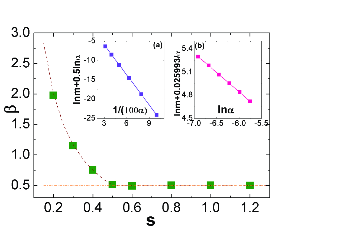
Figure 1: Exponent $\beta$ as a function of $s$ at the parameters: $\Delta=0.1$, $\epsilon=0$, $N_{b}=2$. Dash line represents the analytical data; Olive squares symbol numerical data; Dash-dot line is for $N_{b}=\infty$. The inset shows the magnetization at $s=0$ as a function of $\alpha$ with $N_{c}=2000$.

Similarly, both analytical and numerical results for the critical exponent $\delta$ are available at $N_{b}=2$, as shown in Fig. 2.

$$\delta = \left\{\begin{array}[]{lll}3,&(\textrm{$s\geq\frac{1}{2}$});\\ &\\ \frac{1+s}{1-s},&(\textrm{$0<s<\frac{1}{2}$}).\end{array}\right.$$ (38)

It is noted that in $0<s<1/2$, both $\beta$ and $\delta$ for $N_{b}=2$ agree with the corresponding exponents in the spin-boson model obtained from NRG. A natural question is how the nonclassical critical exponents $\beta$ and $\delta$ in the regime $0<s<1/2$ as given in Eq.(33) and Eq.(38) at $N_{b}=2$ change to classical ones at $N_{b}=\infty$. In the following section, we explore this issue at intermediate $N_{b}$’s.

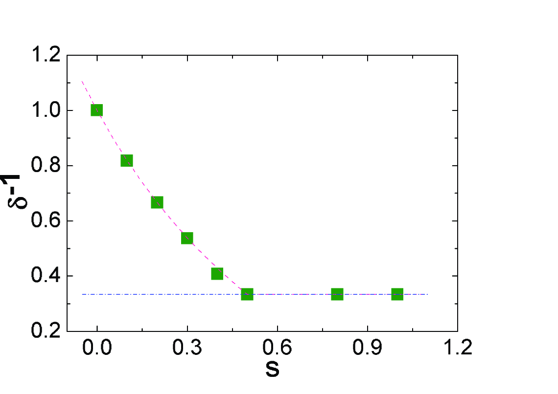
Figure 2: Exponent $\delta^{-1}$ as a function of $s$ at the parameters: $\Delta=0.1$, $\alpha=\alpha_{c}$, $N_{b}=2$. The dash line is the analytical result; The olive squares are numerical data; The dash-dot line is for $N_{b}=\infty$.

3.3 Numerical analysis at intermediate $N_{b}$’s

At intermediate $N_{b}$’s, we calculate $<a_{n}+a_{n}^{{\dagger}}>$ by exact diagonalization and solve the mean-field equation iteratively. For $s\geq 1/2$, the numerical results always yield the classical critical exponents $\beta=1/2$ and $\delta=3$, irrespective of the boson state truncation $N_{b}$’s. But for $0<s<1/2$, this is no longer the case. In Fig.3, we plot the dependence of the average magnetization $m$ on the dissipation strength $\alpha$ for $s=0.2$, at different $N_{b}$’s ($2\leq N_{b}\leq\infty$). $\alpha_{c}$ is calculated from Eq.(29) at given parameters. It is clearly seen that in the small $\alpha-\alpha_{c}$ limit, $m$ exhibits a perfect power law and the slope $\beta_{d}$ is identical to that of $N_{b}=2$, namely $\beta_{d}=(1-s)/(2s)$, deviating from the classical exponent dramatically. Only for $N_{b}\rightarrow\infty$ do we recover the anticipated mean-field result. In the upper region of the curve, the magnetization at finite but large $N_{b}$ tends to overlap with that at $N_{b}=\infty$, giving a different slope $\beta_{u}=1/2$. As a result, two different power laws appear in the lower and upper regimes of the curve. In the following, we carry out a scaling analysis for $m$ data with respect to parameters $\tau=\alpha-\alpha_{c}$ and $x=1/N_{b}$ on the basis of the generalized homogeneous function (setting $\epsilon=0$) RefAH:25 .

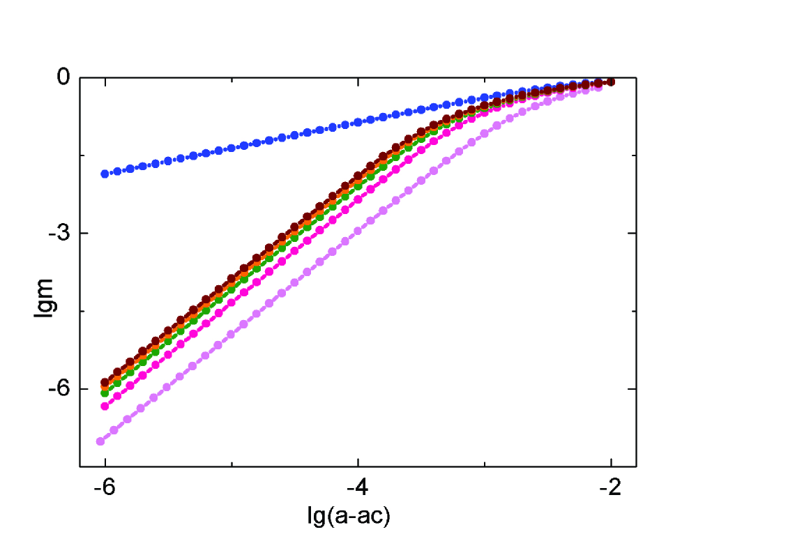
Figure 3: lg$m$ v.s. lg$\tau$ for different truncations at the parameters: $\Delta=0.1$, s=0.2, $\epsilon$=0.0. The truncations are $N_{b}$=2, 5, 10, 15, 20 and $\infty$ from bottom to top.

We assume that the singular part of $m$ is a GHF of $\tau$ and $x$. That is,

$$m(\lambda^{a_{\tau}}\tau,\lambda^{a_{x}}x) = \lambda^{a_{m}}m(\tau,x).$$ (39)

Here $\lambda$ is a positive number. Taking a logarithmic form of the equation above, we arrive at the following:

$$\overline{m}(\overline{\tau}+a_{\tau}\overline{\lambda},\overline{x}+a_{x}\overline{\lambda}) = \overline{m}(\overline{\tau},\overline{x})+a_{m}\overline{\lambda},$$ (40)

where $\overline{i}$=lg$i$, $i=m$, $\tau$, $x$, $\lambda$. This equation implies that if $\overline{m}$, $\overline{\tau}$ and $\overline{x}$ are shifted by $\Delta\overline{m}$, $\Delta\overline{\tau}$, $\Delta\overline{x}$, respectively, the curves will collapse. The ratios of the shifts give the critical exponents $\Delta\overline{m}/\Delta\overline{\tau}=a_{m}/a_{\tau}$ and $\Delta\overline{m}/\Delta\overline{x}=a_{m}/a_{x}$. Assigning $\overline{\lambda}=-\overline{x}/a_{x}$ in Eq.(40), we get

$$\overline{m}(\overline{\tau}-\frac{a_{\tau}}{a_{x}}\overline{x},0) = \overline{m}(\overline{\tau},\overline{x})-\frac{a_{m}}{a_{x}}\overline{x}.$$ (41)

For simplicity, we denote $z=\overline{\tau}-\frac{a_{\tau}}{a_{x}}\overline{x}$. Fig. 3 suggests that we can assume a universal function as:

$$\overline{m}(\overline{\tau}-\frac{a_{\tau}}{a_{x}}\overline{x},0)=\overline{m}(z,0)=\left\{\begin{array}[]{lll}\beta_{u}z+C_{u},&(z\gg z_{0});\\ &\\ \beta_{d}z+C_{d},&(z\ll z_{0}).\end{array}\right.$$ (45)

$z_{0}$ is some crossover value separating two regimes with different power laws. This gives

$$\overline{m}(\overline{\tau},\overline{x})=\left\{\begin{array}[]{lll}\beta_{u}\overline{\tau}+\overline{x}(\frac{a_{m}}{a_{x}}-\frac{a_{\tau}}{a_{x}}\beta_{u})+C_{u},&(\tau^{\frac{1}{a_{\tau}}}\gg cx^{\frac{1}{a_{x}}});\\ &\\ \beta_{d}\overline{\tau}+\overline{x}(\frac{a_{m}}{a_{x}}-\frac{a_{\tau}}{a_{x}}\beta_{d})+C_{d},&(\tau^{\frac{1}{a_{\tau}}}\ll cx^{\frac{1}{a_{x}}}).\end{array}\right.$$ (49)

$C_{u}$, $C_{d}$ and $c$ are constants. The truncation independence of the upper power in Fig. 3 requires that the coefficient of $\overline{x}$ in $\tau^{\frac{1}{a_{\tau}}}\gg cx^{\frac{1}{a_{x}}}$ regime should be zero, namely $a_{m}/a_{x}=\beta_{u}a_{\tau}/a_{x}$ or $\beta_{u}=a_{m}/a_{\tau}$. In the small $\tau$ regime, Fig. 3 suggests that at finite truncations, $\beta_{d}$ is identical to that of $N_{b}=2$, namely $\beta_{d}=(1-s)/(2s)$.

Our assumptions in Eq.(49) are verified in Fig. 4(a). All the curves overlap with the curve at $N_{b}=10$ after proper translations of $\overline{m}$ and $\overline{\tau}$. Translation details are in Tab. 1. We get $\Delta\overline{m}/\Delta\overline{\tau}=a_{m}/a_{\tau}\simeq 0.5$, supporting $\beta_{u}=\beta_{MF}=1/2$, consistent with the specific case $N_{b}=\infty$. According to Eq.(49), the crossover point $\tau_{cr}$ between the two power law regime $\beta_{u}=1/2$ (upper power) and $\beta_{d}=(1-s)/(2s)$ (lower power) is given by $\tau_{cr}\sim x^{a_{\tau}/a_{x}}$. $\tau_{cr}$ declines as $N_{b}$ increases, leading to the expansion of the $\beta_{u}=1/2$ regime. In the limit $N_{b}=\infty$, i.e., $x=0$, $\tau_{cr}$ is moved to zero, and the full mean field curve should be recovered. This is indeed observed in Fig. 3.

Table 1: Translation of $\overline{m}$, $\overline{\tau}$ and $\overline{x}$ data to $N_{b}=10$ curve for $s=0.3$.

$N_{b}$	$\Delta\overline{x}$	$\Delta\overline{\tau}$	$\Delta\overline{m}$	$a_{m}/a_{x}$	$a_{\tau}/a_{x}$	$a_{m}/a_{\tau}$
15	0.176	0.20	0.10	0.57	1.14	0.50
20	0.301	0.30	0.15	0.50	1.00	0.50
30	0.477	0.48	0.24	0.50	1.00	0.50
40	0.602	0.60	0.29	0.48	1.00	0.48
80	0.903	0.86	0.43	0.48	0.95	0.50

In the regime $\tau<\tau_{cr}$, the second equation in Eq.(49) holds. Fig. 4(b) shows lg$m-\beta_{d}$lg$\tau$ v.s. lg$x$ at fixed $\tau$ in the lower regime. Here $\beta_{d}=(1-s)/(2s)$ is used. For various $s$ values, the curves are linear with the same slope $C$. This confirms the second equation of Eq.(49) and gives $\beta_{d}a_{\tau}/a_{x}-a_{m}/a_{x}=C$, being independent of $s$. Numerical fitting gives the slope $C\sim 0.61\pm 0.02$. Taking into account of $a_{m}/a_{\tau}=1/2$ and $\beta_{d}=(1-s)/(2s)$, we get

$$\frac{a_{\tau}}{a_{x}} = \frac{2Cs}{1-2s},$$ (50)

$$\frac{a_{m}}{a_{x}} = \frac{Cs}{1-2s}.$$ (51)

They are plotted as lines in Fig. 5. On the other hand, the average values of $a_{m}/a_{x}$ and $a_{\tau}/a_{x}$ obtained from translation of $\overline{m}$ data are plotted in Fig. 5 as functions of $s$. They match Eq.(50) and Eq.(51) remarkably well.

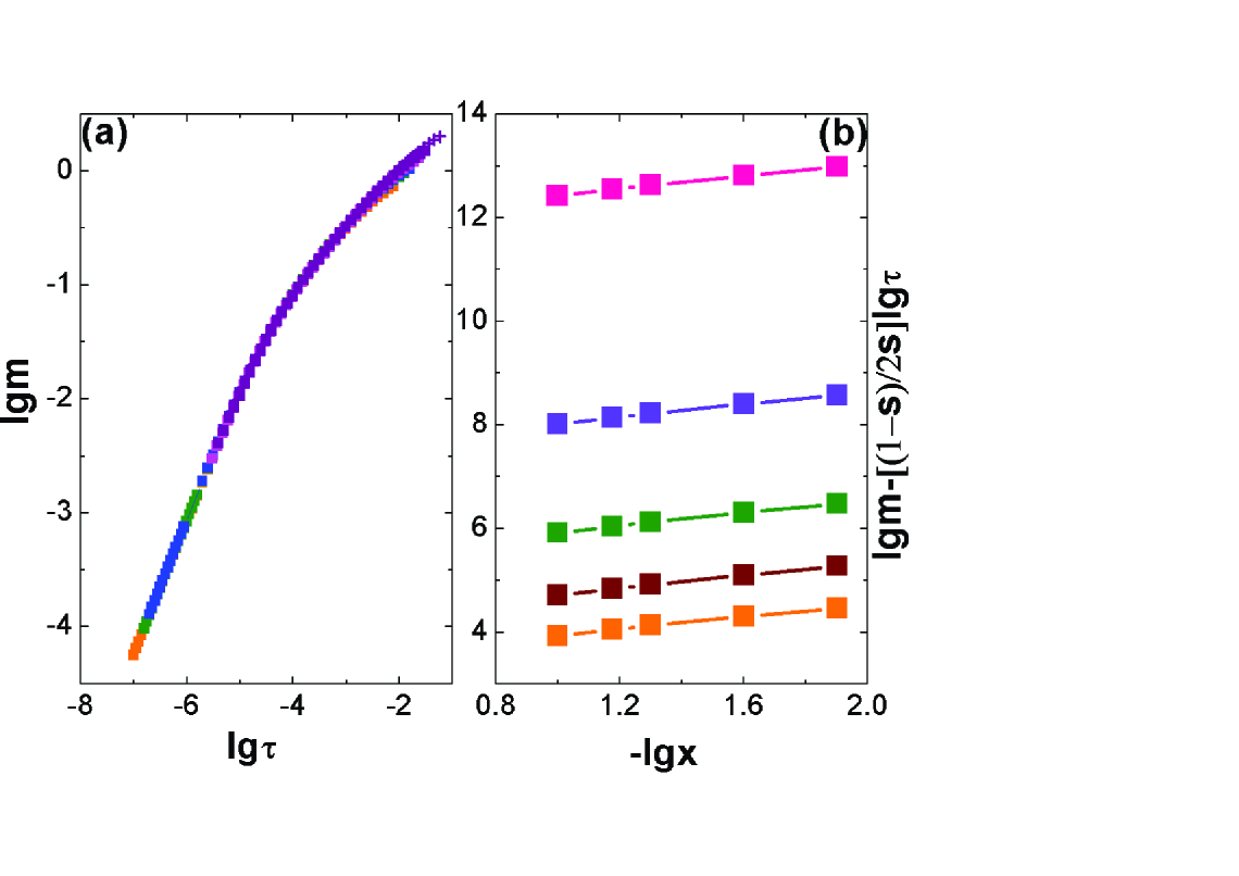
Figure 4: (a) Overlap of curves with $N_{b}=15,20,30,40,80$ to the curve with $N_{b}=10$ after proper translation at $s=0.3$. (b) Scaling of the magnetization with respective to the truncation. From top to bottom $s=0.1,0.15,0.2,0.25,0.3$, respectively. Here, we use lg$\tau$= -5.0 for $s=0.1$ and lg$\tau$=-6.0 for the others. Parameters are $\Delta$=0.1, $\epsilon$=0.0.

Fig.(1)-(4) show that even for a mean-field Hamiltonian, local boson state truncation can dramatically alter the critical exponents, from the Gaussian exponents to the interacting ones. The boson state truncation, i.e., the artificial constraint of the local Hilbert space can be regarded as an additional local interaction introduced between bosons. For the mean-field model with Gaussian critical fixed point, this interaction becomes dominant in low energies and leads the system to a new interacting critical fixed point. The critical exponent does not change continuously with the Hilbert space constraint. Instead, the constraint tunes the crossover point in the $m-\tau$ curve below which the system flows into a truncation-dominated interacting fixed point.

Our results shed some lights on the problem of bosonic NRG for the spin-boson model. That $\beta_{d}=(1-s)/(2s)$ of $H_{MF}^{star}$ agrees with the $\beta$ obtained from NRG for the spin-boson model suggests that $\beta_{d}$ itself is totally dominated by truncation. It is probable that the same scenario of $N_{b}$ also occurs in NRG. If this is true, it becomes clear why the bosonic NRG with boson state truncation cannot give correct classical exponent in this regime: the Gaussian critical fixed point in the regime $0<s<1/2$ is overtaken by the strong relevant operator introduced by the Hilbert space truncation RefVT:16 ; RefVTB:24 . Moreover, one cannot improve the NRG critical exponent simply by increasing $N_{b}$ if one focuses only on the small $\tau$ limit. Instead, the correct exponents can be crudely observed at finite energy scales from the truncated NRG calculation as shown in Ref.RefVTB:24 . As demonstrated here, to fully disclose the role of $N_{b}$ and to extract the accurate exponent $\beta$ from the bosonic NRG calculation, it is necessary to carry out a scaling analysis of $N_{b}$. It is worth mentioning that the NRG study of the Ising-BFKM gives the interacting critical fixed point in the regime $0<s<1/2$, in contrast to the belief that the Ising-BFKM and SBM belong to the same universality class RefTI:26 ; RefMK:27 . In light of our study, we suggest that the NRG study for Ising-BFKM should be checked, using similar scaling analysis of $N_{b}$.

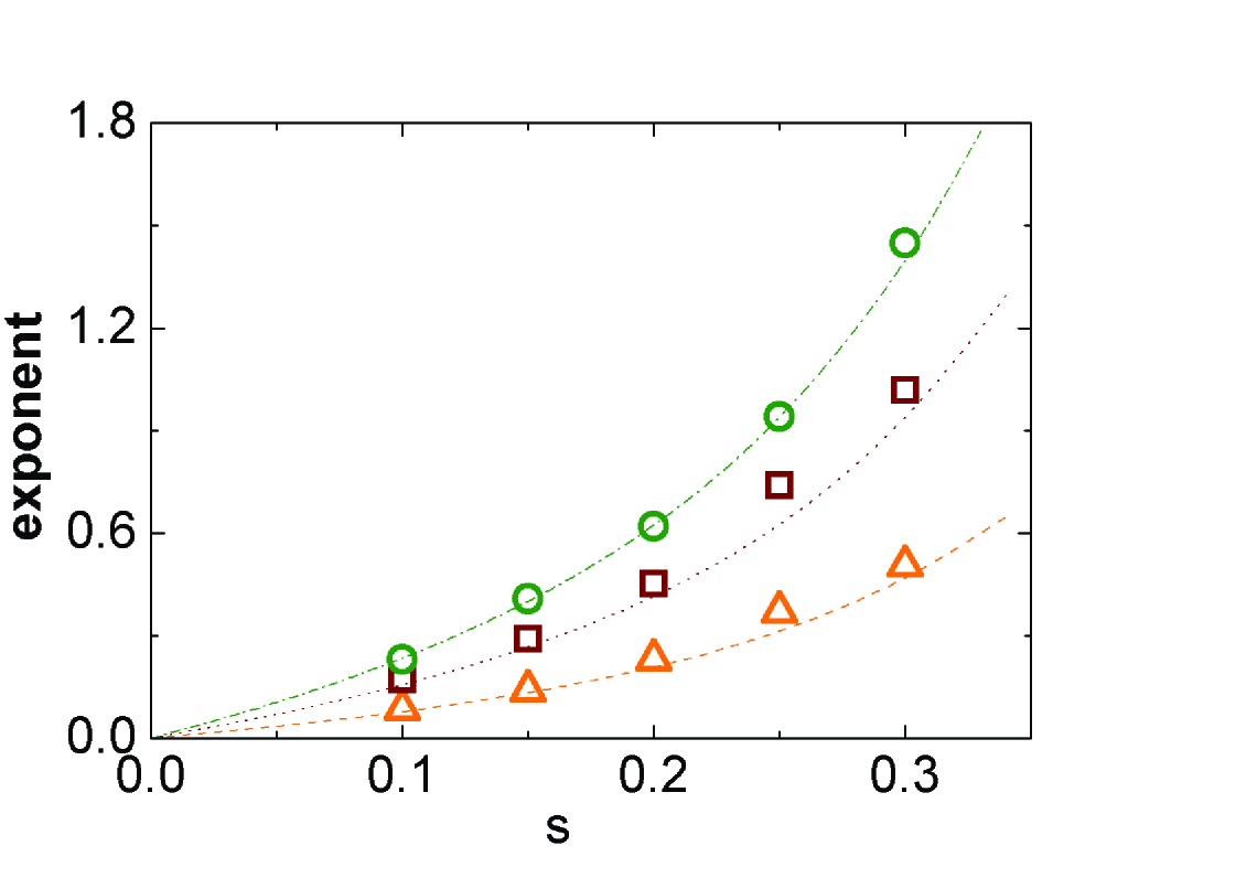
Figure 5: Ratio of the scaling powers as functions of $s$ at $\Delta=0.1$. Orange triangles are $a_{m}/a_{x}=\Delta\overline{m}/\Delta\overline{x}$ obtained from translation in lg$m$ v.s. lg$\tau$ figures at different $s$’s as Fig. (4.a) for $s=0.3$; Dash line is the function $a_{m}/a_{x}=-0.61s/(2s-1)$. Wine squares are $a_{\tau}/a_{x}=\Delta\overline{\tau}/\Delta\overline{x}$ from translation in lg$m$ v.s. lg$\tau$ figures at different $s$’s like Fig. (4.a); The dot line is $-1.22s/(2s-1)$. Olive circles are $a_{\epsilon}/a_{x}$ from translation in lg$m$ v.s. lg$\epsilon$ figures at different $s$’s as Fig. (6.b) for $s=0.2$; The dash-dot line is $-1.83s/(2s-1)$.

In the following, we study the influence of truncation on $\delta$. In Fig. 6, we show $m$ as a function of bias $\epsilon$ at the critical $\alpha_{c}$’s with different $N_{b}$’s and the collapse of these curves to the curve at $N_{b}=10$. Fig. 6(a) shows that in the lower regime the magnetization has the same power dependence on $\epsilon$ as that of $N_{b}=2$, i.e., $\delta_{d}=(1+s)/(1-s)$ as given in Eq.(38). Fig. 6(b) shows the collapse of the lg$m$-lg$\epsilon$ curves under proper translations of $\overline{x}$, $\overline{\epsilon}$ and $\overline{m}$. This supports that, near the criticality $m(\epsilon,x)$ is also a GHF:

$$m(\lambda^{a_{\epsilon}}\epsilon,\lambda^{a_{x}}x) = \lambda^{a_{m}}m(\epsilon,x).$$ (52)

The ratios between the shifts are $\Delta\overline{m}/\Delta\overline{\epsilon}=a_{m}/a_{\epsilon}$ and $\Delta\overline{m}/\Delta\overline{x}=a_{m}/a_{x}$. Details of the translation are in Tab. 2. According to Fig. 6(a) and Fig. 6(b), $m$ as a GHF of $x$ and $\epsilon$ can be formulated as:

$$\overline{m}(\overline{\epsilon},\overline{x})=\left\{\begin{array}[]{lll}\delta^{-1}_{u}\overline{\epsilon}+C_{u},&(\epsilon^{\frac{1}{a_{\epsilon}}}\gg cx^{\frac{1}{a_{x}}});\\ &\\ \delta^{-1}_{d}\overline{\epsilon}+\overline{x}(\frac{a_{m}}{a_{x}}-\frac{a_{\epsilon}}{a_{x}}\delta^{-1}_{d})+C_{d},&(\epsilon^{\frac{1}{a_{\epsilon}}}\ll cx^{\frac{1}{a_{x}}}).\end{array}\right.$$ (56)

We get $\delta_{u}^{-1}=a_{m}/a_{\epsilon}=\Delta\overline{m}/\Delta\overline{\tau}\simeq 1/3$, signaling a classical power law in the large $\epsilon$ regime. In Fig. 6(c) we plot $(\overline{m}-\delta_{d}^{-1}\overline{\epsilon})/(a_{m}/a_{x}-\delta_{d}^{-1}a_{\epsilon}/a_{x})$ versus $\overline{x}$ for different $s$. They are linear functions of $\overline{x}$ with an average slope $1.01\pm 0.05$, as expected from the second equation of Eq.(56).

In Fig.5, $a_{\epsilon}/a_{x}$ obtained from the translation procedure is plotted as circles, to be compared with the analytical curve $a_{\epsilon}/a_{x}=3Cs/(1-2s)$. Here we use the value $C=0.61$ obtained previously. They agree very well. These numerical results confirm our assumption in Eq.(56).

Table 2: Translation of $\overline{m}$, $\overline{\epsilon}$ and $\overline{x}$ data to $N_{b}=10$ curve for $s=0.2$.

$N_{b}$	$\Delta\overline{x}$	$\Delta\overline{\epsilon}$	$\Delta\overline{m}$	$a_{m}/a_{x}$	$a_{\epsilon}/a_{x}$	$a_{m}/a_{\epsilon}$
15	0.176	0.11	0.036	0.20	0.63	0.33
20	0.301	0.19	0.063	0.21	0.63	0.33
40	0.602	0.36	0.12	0.20	0.60	0.33
80	0.903	0.56	0.19	0.21	0.62	0.34
100	1.000	0.63	0.21	0.21	0.63	0.33

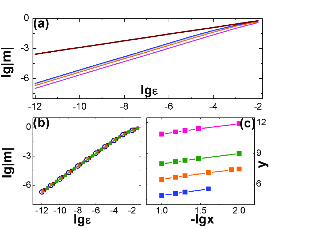
Figure 6: Magnetization $m$ as functions of bias $\epsilon$ for different truncations at the parameters: $\Delta=0.1$, $\alpha=\alpha_{c}$, $s=0.2$. (a) $N_{b}=2,10,40,100,\infty$ from bottom to top. (b) Overlap of curves with $N_{b}=15,20,40,80,100$ to the curve with $N_{b}=10$ after proportional translation. (c) Scaling of the magnetization in terms of the truncation. $s=0.1,0.15,0.2,0.3$ from top to bottom. $y=[\overline{m}-\overline{\epsilon}(1-s)/(1+s)]/[2Cs/(1+s)]$, here we use $\overline{\epsilon}=-9.0$ and $C=0.61$.

This shows that $m(\epsilon,x)$ is also a function with two different power law regimes: the low energy regime with $1/\delta_{d}$ and the upper one with $1/\delta_{MF}=1/3$. They are separated by a crossover point $\epsilon_{cr}\sim x^{a_{\epsilon}/a_{x}}$, similar to the situation in $m(\tau,x)$.

In the following, we discuss the susceptibility exponent $\gamma$. In Fig. 7, $1/\chi$ versus $\alpha$ is plotted. The zero point in the figure is the critical point. Within the critical region, the susceptibility exponent remains the classical one, $\gamma=1$ under finite boson state truncation in $0<s<1/2$. This shows that the boson state truncation does not influence $\gamma$. Similar observations are made in the NRG, MC, SPSA and extended coherent state approach studies RefVT:16 ; RefWR:18 ; RefAAH:19 ; RefYQK:28 .

From the analysis above, we observe that in the low energy regimes, i.e., $\tau^{1/a_{\tau}}\ll cx^{1/a_{x}}$ and $\epsilon^{1/a_{\epsilon}}\ll cx^{1/a_{x}}$, $\beta$ and $\delta$ are no longer determined by the scaling exponents $a_{m}$, $a_{\tau}$, $a_{\epsilon}$. Instead new parameters are needed to define those critical exponents. We also find that in both the high and low energy regimes, the scaling relation $\beta(\delta-1)=\gamma$ is fulfilled.

The same analysis is carried out at a different $\Delta$ and $\Lambda$: $\Delta=0.2$ and $\Lambda=3.0$. Conclusions are qualitatively the same. From the analysis above, we believe that it is not the failure of quantum-to-classical mapping for the spin-boson model, but the numerical concomitant, i.e., the truncation that leads to new exponents in the regime $0<s<1/2$. Our work shows that the boson state truncation $N_{b}$ severely changes the critical behavior of the mean-field spin-boson model: it plays the role of a new scaling parameter and changes the low energy exponent $\beta$ and $\delta$ into a truncation-dominated exponent (Eq.(33) and Eq.(38)).

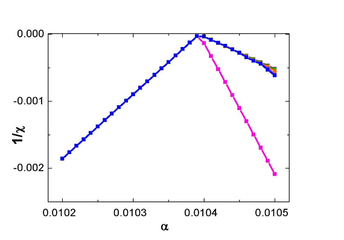
Figure 7: Inverse of susceptibility $1/\chi$ as a function of $\alpha$ for different truncations $N_{b}$ at the parameters: $\Delta=0.1$, s=0.2, $\epsilon=0$. The zero point of $1/\chi$ gives the critical coupling strength $\alpha_{c}$. $N_{b}=2$, 5, 10, 15, 20, 40, 80, 100, $\infty$ from top to bottom, respectively.

4 Summary

To conclude, we have analyzed the mean-field spin boson model under boson state truncation. We focus on the quantum critical behavior of the model and carry out the scaling analysis of the magnetization in terms of truncation parameter $N_{b}$. Our work shows that for the mean field spin boson model the truncation gives rise to a relevant perturbation in the regime $0<s<1/2$. The effect of the truncation, while cutting no ice for the exponents $\beta$ and $\delta$ in the regime $s>1/2$, dominates in $0<s<1/2$. As is shown in in Fig. 3 and in Fig. 6, the magnetization $m$ under truncation is a generalized homogeneous function in the regime $0<s<1/2$: in the high energy regime, $m$ fulfills a classical power law; in the low energy regime it exhibits a double power behavior, and the truncation $N_{b}$ becomes a new scaling parameter, besides the coupling strength $\tau$ and external field $\epsilon$ (Eq.(49) and Eq.(56)). Moreover, we find that as $N_{b}$ increases, the crossover point between two power law regimes moves downwards and to zero energy scale at $N_{b}=\infty$ (namely without boson states truncation). Implications of these findings to the bosonic NRG study are discussed. For the spin-boson model within $0<s<1/2$, it is now believed that the low energy critical exponents $\beta=(1-s)/(2s)$ and $\delta=(1+s)/(1-s)$ obtained by NRG are also due to boson state truncation $N_{b}$ RefVT:16 ; RefVTB:24 . We conjecture that similar scaling behavior of $N_{b}$ should also occur in the NRG study of the spin-boson model. A correct and accurate extraction of $\beta$ and $\delta$ for the spin-boson model from NRG requires similar scaling analysis as done here. Further studies in this direction are in progress.

N. H. Tong acknowledges helpful discussions with Ralf Bulla and Matthias Vojta. This work is supported by National Basic Research Program of China (grant number 2007CB925004), and by the NSFC under grant number 10674178.

Appendix A Appendix

In the Appendix we give the analytical derivation of the critical exponents at $N_{b}=2$. Following similar procedures in Sec. 2.2, we can get the self-consistent equations for the magnetization m at $N_{b}=2$

$$m = \frac{\Delta^{2}-(\epsilon+\epsilon^{\prime}+t)^{2}}{\Delta^{2}+(\epsilon+\epsilon^{\prime}+t)^{2}},$$ (57)

$$t = \sqrt{(\epsilon+\epsilon^{\prime})^{2}+\Delta^{2}},$$ (58)

$$\epsilon^{\prime} = -\frac{m}{\pi}\sum_{n}d_{n},$$ (59)

$$d_{n} = \frac{\gamma_{n}^{2}}{\sqrt{\xi_{n}^{2}+\frac{m^{2}\gamma_{n}^{2}}{\pi}}}.$$ (60)

with $\gamma_{n}$ and $\xi_{n}$ satisfying Eq.(11) and Eq.(12), respectively. Since we are interested in the critical exponent $\beta$, first we take the bias $\epsilon$ to be zero. Combining Eq.(57) and Eq.(58), we get the following equation:

$$m = \frac{\epsilon^{\prime}}{\sqrt{{\epsilon^{\prime}}^{2}+\Delta^{2}}}.$$ (61)

The newly obtained Eq.(61) together with Eq.(59) composes the self-consistent equations. To calculate the summation in Eq.(59), we define a parameter $n_{0}$ determined by the following equation:

$$\xi_{n_{0}}^{2}=\frac{m^{2}\gamma_{n_{0}}^{2}}{\pi}.$$ (62)

Then Eq.(59) can be divided into two parts:

$$\epsilon^{\prime} = -\frac{m}{\pi}[{\sum_{n=0}^{n_{0}}d_{n}+\sum_{n=n_{0}+1}^{\infty}d_{n}}].$$ (63)

When $n\ll n_{0}$, i.e., $\xi_{n}^{2}\gg\frac{m^{2}\gamma_{n}^{2}}{\pi}$,

$$d_{n} = \frac{\gamma_{n}^{2}}{\xi_{n}}(1+\frac{m^{2}\gamma_{n}^{2}}{\pi\xi_{n}^{2}})^{-\frac{1}{2}}$$ (64)

$$= \sum_{k=0}^{\infty}P_{k}\Lambda^{n[k(1-s)-s]}m^{2k}.$$

On the contrary,when $n\gg n_{0}$, i.e., $\xi_{n}^{2}\ll\frac{m^{2}\gamma_{n}^{2}}{\pi}$,

$$d_{n} = \frac{\sqrt{\pi}\gamma_{n}}{m}(1+\frac{\xi_{n}^{2}\pi}{m^{2}\gamma_{n}^{2}})^{-\frac{1}{2}}$$ (65)

$$= \sum_{k=0}^{\infty}Q_{k}\Lambda^{\frac{n[2k(s-1)-1-s]}{2}}m^{-2k-1}.$$

Here, $P_{k}=\frac{C_{k}^{-1/2}}{\pi^{k}}\frac{A^{2k+2}}{B^{2k+1}}$ and $Q_{k}=\frac{C_{k}^{-1/2}\pi^{k+1/2}B^{2k}}{A^{2k-1}}$, with $C_{k}^{-1/2}=-\frac{1}{2}(-\frac{1}{2}-1)...[-\frac{1}{2}-(k-1)]$ ($C_{0}^{-1/2}=1$), $A^{2}=\gamma_{n}^{2}\Lambda^{n(1+s)}$ and $B=\xi_{n}\Lambda^{n}$. Replacing $d_{n}$ in Eq.(63) with Eq.(64) and Eq.(65), respectively, we arrive at the summation:

$$\epsilon^{\prime} = -\frac{m}{\pi}[\sum_{k}P_{k}^{\prime}m^{2k}-Tm^{\frac{2s}{1-s}}].$$ (66)

Here, $P_{k}^{\prime}=P_{k}/[1-\Lambda^{k(1-s)-s}]$. It is hard to get the analytical form for $T$, anyhow, it does not contribute to the exponent of the order parameter. Neglecting the trivial solution $m=0$, we get the following self-consistent equation by substituting $\epsilon^{\prime}$ in Eq.(61) with Eq.(66),

$$[\sum_{k}P_{k}^{\prime}m^{2k}-Tm^{\frac{2s}{1-s}}]^{2}(1-m^{2}) = \pi^{2}\Delta^{2}.$$ (67)

Considering that the order parameter approaches zero near the critical coupling $\alpha_{c}$, we get

$$P_{0}^{\prime}+P_{1}^{\prime}m^{2}-Tm^{\frac{2s}{1-s}} = \pi\Delta.$$ (68)

The final critical coupling strength $\alpha_{c}$ is

$$\alpha_{c} = \frac{\Delta(s+1)^{2}(1-\Lambda^{-s})[1-(\Lambda^{-(s+2)})]}{2\omega_{c}(s+2)[1-(\Lambda^{-(s+1)})]^{2}},$$ (69)

the same as in Eq.(29) for $N_{b}=\infty$. For $s>1/2$, the third term in Eq.(68) is negligible and one gets $m\propto(\alpha-\alpha_{c})^{1/2}$; for $s=1/2$, the second and third term have the same power, i.e., $(1-s)/(2s)=1/2$ (s=1/2), so one gets $m\propto(\alpha-\alpha_{c})^{1/2}$; for $0<s<1/2$, ignoring the second term in Eq.(68), one gets $m\propto(\alpha-\alpha_{c})^{(1-s)/(2s)}$. In summary, for $N_{b}=2$, we get

$$\beta = \left\{\begin{array}[]{lll}\frac{1}{2},&(\textrm{$s\geq\frac{1}{2}$});\\ &\\ \frac{1-s}{2s},&(\textrm{$0<s<\frac{1}{2}$}).\end{array}\right.$$ (73)

In the case of $s=0$, a small difference lies in Eq.(64) at $k=0$. If $s=0$ and $k=0$, the common ratio of the geometric series in Eq.(63) for $n<n_{0}$, namely $\Lambda^{[k(1-s)-s]}$, is unity and the general summation formula is not applicable. Taking this speciality into account and following similar procedure of the case $s\neq 0$, one gets the critical behavior of the magnetization as

$$m\propto\alpha^{-\frac{1}{2}}e^{-\frac{\Delta ln\Lambda(1+\Lambda^{{}^{-1}})}{8\alpha\omega_{c}(1-\Lambda^{-1})}}.$$ (74)

As far as $\delta$ is concerned, similar analysis gives the following expression

$$\delta = \left\{\begin{array}[]{lll}3,&(\textrm{$s\geq\frac{1}{2}$});\\ &\\ \frac{1+s}{1-s},&(\textrm{$0<s<\frac{1}{2}$}).\end{array}\right.$$ (78)

References

- (1) U. Weiss, Quantum Dissipative Systems (World Scientific, Singapore 1993).
- (2) A. J. Leggett, S. Chakravarty, A. T. Dorsey, M. P. A. Fisher, A. Garg and W. Zwerger, Rev. Mod. Phys. 59, 1 (1987).
- (3) F. Verstraete, D. Porras and J. I. Cirac, Phys. Rev. Lett. 93, 227205 (2004).
- (4) J. S. Pentill, U. Parks, P. J. Hakonen, M. A. Paalanen, and E. B. Sonin, Phys. Rev. Lett. 82, 1004 (1999).
- (5) T. Hayashi, T. Fujisawa, H.D . Cheng, Y. H. Jeong, and Y. Hirayama, Phys. Rev. Lett. 91, 226804 (2003).
- (6) D. Porras, F. Marquardt, J. von Delft, and J.I . Cirac, Phys. Rev. A. 78, 010101(R) (2008).
- (7) N. H. Tong and M. Vojta, Phys. Rev. Lett. 97, 016802 (2006).
- (8) F. J. Dyson, Commun. Math. Phys. 12, 91 (1969).
- (9) M. E. Fisher , Phys. Rev. Lett. 29, 917 (1972)
- (10) E. Luijten and H. W. J. Blte, Phys. Rev. B. 56, 8945 (1997)
- (11) S. K. Kehrein and A. Mielke, Phys. Lett. A. 219, 313 (1996).
- (12) T. Stauber and A. Mielke, Phys. Lett. A. 305, 275 (2002).
- (13) T. Stauber, Phys. Rev. B. 68, 125102 (2003).
- (14) Z. Lu and H. Zheng, Phys. Rev. B. 75, 054302 (2007).
- (15) R. Bulla, N. H. Tong and M. Vojta, Phys. Rev. Lett. 91, 170601 (2003).
- (16) M. Vojta, N. H. Tong and R. Bulla, Phys. Rev. Lett. 94, 070604 (2005).
- (17) R. Bulla, H. J. Lee, N. H. Tong, and M. Vojta, Phys. Rev. B. 71, 045122 (2005).
- (18) A. Winter, H. Rieger, M. Vojta and R. Bulla, Phys. Rev. Lett. 102, 030601 (2009).
- (19) A. Alvermann and H. Fehske, Phys. Rev. Lett. 102, 150601 (2009).
- (20) S. Kirchner and Q. Si, arXiv:0808.2647v1[cond-mat.str-el] (2008).
- (21) S. Kirchner and Q. Si , Physica B, 404 2904 (2009).
- (22) S. Kirchner, Q. Si and K. Ingersent, Phys. Rev. Lett. 102, 166405 (2009).
- (23) W. J. Hu and N. H. Tong, Phys. Rev. B. 80, 245110 (2009).
- (24) M. Vojta, N. H. Tong and R. Bulla, Phys. Rev. Lett. 102, 249904 (2009).
- (25) A. Hankey and H. E. Stanley, Phys. Rev. B. 6, 3515 (1972).
- (26) M. T. Glossop and K. Ingersent, Phys. Rev. Lett. 95, 067202 (2005).
- (27) M. T. Glossop and K. Ingersent, Phys. Rev. B 75, 104410 (2007).
- (28) Y. Y. Zhang , Q. H. Chen and K. L. Wang, Phys. Rev. B 81, 121105 (2010).