Integrating Structured Metadata with Relational Affinity Propagation

Abstract

Structured and semi-structured data describing entities, taxonomies and ontologies appears in many domains. There is a huge interest in integrating structured information from multiple sources; however integrating structured data to infer complex common structures is a difficult task because the integration must aggregate similar structures while avoiding structural inconsistencies that may appear when the data is combined. In this work, we study the integration of structured social metadata: shallow personal hierarchies specified by many individual users on the Social Web, and focus on inferring a collection of integrated, consistent taxonomies. We frame this task as an optimization problem with structural constraints. We propose a new inference algorithm, which we refer to as Relational Affinity Propagation (RAP) that extends affinity propagation (?) by introducing structural constraints. We validate the approach on a real-world social media dataset, collected from the photosharing website Flickr. Our empirical results show that our proposed approach is able to construct deeper and denser structures compared to an approach using only the standard affinity propagation algorithm.

Introduction

Structured and semi-structured data describing entities, relationships among entities, and taxonomies and ontologies over them, appear in many domains. There is a great deal of interest in integrating structured information from multiple sources. Some of the areas that have seen much active research include bioinformatics, aggregation services for commercial products and services, and more traditional enterprise database integration. Integrating structured data to infer complex common structures is a difficult task because the integration must aggregate similar structures while avoiding structural inconsistencies that may appear when the data is combined.

This problem becomes even more challenging when one is attempting to integrate numerous, heterogeneous metadata fragments, generated by multiple users. This data is inherently noisy and inconsistent, and there is certainly no single, unified structure to be found. On the other hand, finding and extracting the best exemplar or a set of good example structures can be highly beneficial.

In folksonomy learning (?), structured metadata in the form of hierarchies of concepts created by many users on the Social Web is combined into a global hierarchy of concepts, that reflects how a community organizes knowledge. Users who create personal hierarchies to organize their content may use idiosyncratic categorization schemes (?) and naming conventions. Simply combining nodes with similar names is likely to lead to ill-structured graphs containing loops and shortcuts (multiple paths from one node to another), rather than a taxonomy.

In this paper, we present a probabilistic approach for aggregating relational data into a desired structure. Specifically, our task is to integrate many shallow personal hierarchies, namely saplings, into a deeper, more complete taxonomy. Our learning method, relational affinity propagation, extends affinity propagation (?) by introduces structural constraints that encourages the integration process to combine saplings into trees rather than an arbitrary graph containing loops and shortcuts. We show that embedding the constraints into the hierarchy learning process results in a more accurate merging of saplings that leads to a more consistent tree. We demonstrate the utility of the proposed approach on real-world data extracted from the photosharing site Flickr. Specifically, we combine shallow personal hierarchies created by Flickr users into common deeper hierarchies of concepts.

The objective of the optimization is to combine these small shallow hierarchies into a small number of, deeper and denser hierarchies that represent how a community of users organizes their knowledge. This differs from classical taxonomy and ontology alignment settings (?) where there are typically just a few structures to align, and those structures are large with rich and deep structure and semantics; here we focus on the much messier setting, where we have many small fragments, created by end users with a variety of purposes in mind. In these settings, coming up with a single integrated taxonomy is infeasible, so instead we focus on constructing a small number of useful taxonomies.

We motivate our approach with an example of learning a common taxonomy of concepts from shallow personal hierarchies (saplings) created by many users and illustrate some of the challenges that arise during this task. We then briefly describe how saplings are represented through social annotation on Flickr. We subsequently review the standard affinity propagation algorithm and describe our relational extension to it. Finally, we apply the method to real data sets and show that the proposed approach is able to learn better, and more complete trees.

Motivating Example

We take as our motivating example user-generated annotations on the Social Web. We assume that groups of users share common conceptualizations of the world, which can be represented as a taxonomy or hierarchy of concepts. Figure 1(a) depicts one such common conceptualization about ‘animal’ and its ‘bird’ subconcepts shared by a group of users. When users organize the content they create, e.g., photographs on Flickr, they select some portions of the common taxonomy for categorization. We observe these categories through the shallow personal hierarchies Flickr users create, which we refer to as saplings. Figure 1(b) depicts some of the saplings specified by different users to organize their ‘animal’ and ‘bird’ images. Our ultimate goal is to infer common conceptual hierarchies from the many individual saplings. One natural solution is to aggregate saplings shown in Figure 1(b) together into a deeper and bushier tree shown in Figure 1(a).

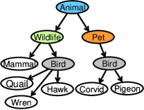
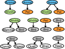
(a)	(b)

Figure 1: Illustrative examples on (a) a commonly shared conceptual categorization (hierarchy) by various users; (b) personal hierarchies expressed by the users based on the conceptual categorization as in (a). Nodes with similar name have similar color just for an illustrative purpose.

To aggregate saplings, we need a combining strategy that measures the degree to which two sapling nodes should or should not be merged. Suppose that we have a very simple combining strategy that says two nodes are similar if they have similar names as in the prior work (?). From Figure 1(b), we will end up with a graph containing one loop and two paths from ‘animal’ to ‘bird’, rather than the tree shown in Figure 1(a). Suppose that we can also access tags with which users annotated photos within saplings, and that photos within “domestic bird” nodes have tags like “pet,” and “farmed” in common, and photos belonging to “wild bird” nodes have tags like “wildlife” and “forest” in common. A cleverer similarity function that, in addition to node names, takes tag statistics within a node into consideration, should split ‘bird’ nodes into two different groups: ‘domestic bird’ and ‘wild bird’, which are put under “pet” and “wildlife” nodes respectively.

The similarity function plays a crucial part in integrating saplings, and a sophisticated enough similarity function that can differentiate node senses in detail, may potentially correctly integrate the final tree. Nevertheless, finding and tuning such function is very difficult; moreover, the data is often inconsistent, noisy and incomplete, especially on the Social Web, where data is generated by many different users.

One possible way to tackle this challenge is to use a simple similarity function and incorporate constraints during the merging process. Intuitively, we would not consider merging the ‘bird’ node under ‘pet’ with the one under ‘wildlife’ because it will result in multiple paths from ‘animal’. These structural constraints are used during sapling aggregation process to ensure that the learned structure is a tree. Specifically, the constraints prevent two nodes from being merged if (1) this will lead to links from different parent concepts or (2) this will lead to an incoming link to the root node of a tree. These constraints guarantee that there is, at most, a single path from one node to another.

Structured Metadata in Flickr

Structured data in the form of shallow hiearchies is ubiquitous on the Social Web. On Flickr, users can arbitrarily group related photos into sets and then group related sets in collections. Some users create multi-level hierarchies containing collections of collections, etc., but the vast majority of users who use collections create shallow hierarchies, consisting of collections and their constituent sets. These personal hierarchies generally represent subclass and part-of relationships.

We formally define a sapling as a shallow tree representing a personal hierarchy which composed of a root node $r^{i}$ and its children, or leaf, nodes $\langle l^{i}_{1},..l^{i}_{j}\rangle$. The root node corresponds to a user’s collection, and inherits its name, while the leaf nodes correspond to the collection’s constituent sets and inherit their names. We assume that hierarchical relations between a root and its children, $r^{i}\rightarrow l^{i}_{j}$, specify broader-narrower relations.

On Flickr, users can attach tags only to photos. A sapling’s leaf node corresponds to a set of photos, and the tag statistics of the leaf are aggregated from that set’s constituent photos. Tag statistics are then propagated from leaf nodes to the parent node. We define a tag statistic of node $x$ as $\tau_{x}:=\{(t_{1},f_{t_{1}}),(t_{2},f_{t_{2}}),\cdots(t_{k},f_{t_{k}})\}$, where $t_{k}$ and $f_{t_{k}}$ are tag and its frequency respectively. Hence, $\tau_{r^{i}}$ is aggregated from all $\tau_{l^{i}_{j}}$s. These tag statistics can also be used as a feature for determining if two nodes are similar (of the same concept).

Affinity Propagation

A key component of folksonomy learning through sapling integration is the merging similar nodes in different saplings. Merging similar root nodes expands the width of the learned tree, while merging the leaf of one sapling to the root of another extends the depth of the learned tree. We cast the merging process as clustering sapling nodes, and we use affinity propagation to perform the clustering. Below, we briefly review the original AP and then describe our extension, which incorporates structural constraints, and refer to the extended version as Relational Affinity Propagation (RAP).

Affinity Propagation(AP)

Affinity Propagation (?) is a clustering algorithm that identifies a set of exemplar points that are representative of all the points in the data set. The exemplars emerge as messages are passed between data points, with each point assigned to an exemplar. AP attempts to find the exemplar set which maximizes the net similarity, or the overall sum of similarities between all exemplars and their data points.

In this paper, we describe AP in terms of a factor graph (?) on binary variables, as recently introduced by Givoni and Frey (?). The model is comprised of a square matrix of binary variables, along with a set of factor nodes imposed on each row and column in the matrix. Following the notations defined in the original paper (?), let $c_{ij}$ be a binary variable. $c_{ij}=1$ indicates that node $i$ belongs to node $j$ (or, $j$ is an exemplar of $i$); otherwise, $c_{ij}=0$. Let $N$ be a number of data points; consequently, the size of the matrix is $N\times N$.

There are two types of constraints that enforce cluster consistency. The first type, $I_{i}$, which is imposed on the row $i$, indicates that a data point can belong to only one exemplar ($\sum_{j}{c_{ij}}=1$). The second type, $E_{j}$, which is imposed on the column $j$, indicates that if a point other than $j$ chooses $j$ as its exemplar, then $j$ must be its own exemplar ($c_{jj}=1$). AP avoids forming exemplars and assigning cluster memberships which violate these constraints. Particularly, if the configuration at row $i$ violates $I$ constraint, $I_{i}$ will become $-\infty$ (and similarly for $E_{j}$).

In addition to the constraints, there is a similarity function $S(.)$, which indicates how similar a certain node is, to its exemplar. If $c_{ij}=1$, then $S(c_{ij})$ is a similarity between nodes $i$ and $j$; otherwise, $S(c_{ij})=0$. $S(c_{jj})$ evaluates “self-similarity,” also called “preference”, which should be less than the maximum similarity value in order to avoid all singleton points becoming exemplars. This is because that configuration yields the highest net similarity. In general, the higher the value of the preference for a particular point, the more likely that point will become an exemplar. In addition, we can set the same self-similarity value to all data points, which indicates that all points are equally likely to be formed as exemplars.

(a)	(b)

Figure 2: The original binary variable model for Affinity Propagation proposed by Givoni and Frey(?): (a) a matrix of binary hidden variables (circles) and their factors(boxes); (b)incoming and outgoing messages of a hidden variable node from/to its associated factor nodes.

A graphical model for affinity propagation is depicted in Figure 2, described in terms of a factor graph. In a log-form, the global objective function, which measures how good the present configuration (a set of exemplars and cluster assignments) is, can be written as a summation of all local factors as follows:

$$\textbf{S}(c_{11},\cdots,c_{NN}) = \sum_{i,j}S_{ij}(c_{ij})+\sum_{i}I_{i}(c_{i1},\cdots,c_{iN})$$ (1)

$$+ \sum_{j}E_{j}(c_{1j},\cdots,c_{1N}).$$

That is, optimizing this objective function finds the configuration that maximizes the net similarity $S$, while not violating $I$ and $E$ constraints.

The original work uses max-sum algorithm to optimize this global objective function, and it requires updating and passing five messages as shown in Figure 2(b). Since each hidden node $c_{ij}$ is a binary variable (two possible values), one can pass a scalar message — the difference between the messages when $c_{ij}=1$ and $c_{ij}=0$, instead of carrying two messages at a time. The equations to update these messages are described in greater detail in the Section 2 of the original work (?).

Once the inference process terminates, the MAP configuration (exemplars and their members) can be recovered as follows. First, identify an exemplar set by considering the sum of all incoming messages of each $c_{jj}$ (each node in the diagonal of the variable matrix). If the sum is greater than $0$ (there is a higher probability that node $j$ is an exemplar), $j$ is an exemplar. Once a set of exemplars $K$ is recovered, each non-exemplar point $i$ is assigned to the exemplar $k$ if the sum of all incoming messages of $c_{ik}$ is the highest compared to the other exemplars.

Relational Affinity Propagation(RAP)

We extend the above algorithm to add in structural constraints that will ensure that the learned folksonomy makes sense – no loops, and, to the extent possible, forms a taxonomy. In fact, here, we require it to be a tree. Since we want the learned folksonomy to be a tree, all nodes assigned to some exemplar must have their incoming links from nodes in the same cluster, i.e., assigned to the same exemplar. To achieve this, we must enforce the following two constraints: (1) merging should not create incoming links to a cluster, or concept, from more than one parent cluster (single parent constraint); (2) merging should not create an incoming link to the root of the induced tree (no root parent constraint). For the second constraint, we can simply discard all sapling leaves that are named similar to the tree root. Hence, we only need to enforce the first constraint. The first constraint will be violated if leaf nodes of two saplings are merged, i.e., assigned to the same exemplar, while the root nodes of these saplings are assigned to different exemplars. Consequently, the leaf cluster will have multiple parents pointing to it, which leads to an undesirable configuration.

Let $pa(.)$ be a function that returns the index of the parent node of its argument, and $explr(.)$ be a function that return the index of the argument’s exemplar. The factor $F$, “single parent constraint”, checks the violation of multiple parent concepts pointing to a given concept. The constraint is formally defined as follows:

$$F_{j}(c_{1j},\cdots,c_{Nj})=\left\{\begin{array}[]{l l}-\infty&\quad\mbox{$\exists i,k:c_{ij}=1$;$c_{kj}=1$;}\\ &\mbox{$explr(pa(i))\neq explr(pa(k))$,}\\ 0&\quad\mbox{otherwise.}\end{array}\right.$$ (2)

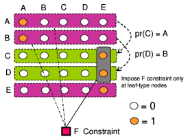
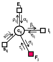
(a)	(b)

Figure 3: The Relational Affinity Propagation proposed in this paper: (a) a schematic diagram of the matrix of binary hidden variables(circles), and variables within the green shade corresponding to some leaf nodes; while those within the pink shade corresponding to some root nodes of some saplings. (b) incoming and outgoing messages of a hidden variable node from/to its associated factor nodes. There are two more messages $\sigma$ and $\tau$. Note that for (a), we omit $E$, $I$ and $S$ factors simply for the sake of clarity.

Figure 3(a) illustrates the way we impose the new constraint on the binary variable matrix. The configuration shown in the figure is valid since both $C$ and $D$ belong to the same exemplar $E$ and their respective parents, $A$ and $B$, belong to the same exemplar $A$. However, if $c_{BB}=1$, then the configuration is invalid, because parents of nodes in the cluster of exemplar $E$ will belong to different exemplars. This constraint is imposed only on leaf nodes, because merging root nodes will never lead to multiple parents. The global objective function for Relational Affinity Propagation is basically Eq. (1) plus $\sum_{j}F_{j}(c_{1j},\cdots,c_{Nj})$.

We modify the equations for updating the messages $\rho$, $\beta$ and also derive $\sigma$ and $\tau$ to take into account this additional constraint. Following the max-sum message update rule from a variable node to a factor node (cf., eq. 2.4 in Chapter 8 of (?)), the message update formulas for $\rho$, $\beta$ and $\sigma$ are simply:

$$\rho_{ij}=S(i,j)+\eta_{ij}+\tau_{ij},$$ (3)

$$\beta_{ij}=S(i,j)+\alpha_{ij}+\tau_{ij},$$ (4)

$$\sigma_{ij}=S(i,j)+\alpha_{ij}+\eta_{ij}.$$ (5)

For deriving the message update equation for $\tau$, we have to consider two cases: $i=j$ and $i\neq j$, i.e., the $\tau$ message to the nodes on the diagonal and $\tau$ for the others. For simplicity, we also assume that all leaf nodes have their index numbers less than any roots. Let $L$ be a number of leaf nodes. Hence, leaf node indices run from $1$ to $L$.

For the case $i=j$ (for the diagonal nodes $c_{jj}$), we have to consider the update message for $\tau$ in two possible settings: $c_{jj}=1$ and $c_{jj}=0$ (or, they can be written as $\tau_{jj}(1)$ and $\tau_{jj}(0)$ respectively), and then find the best configuration for these settings. Following the max-sum message update rule from a factor node to a variable node (cf., eq. 2.5 in Chapter 8 of (?), when $c_{jj}=1$:

$$\tau_{jj}(1)=\max_{\texttt{S}^{j}}\{\sum_{k\in\texttt{S}^{j};k\neq j}{\sigma_{kj}(1)}+\sum_{l\notin\texttt{S}^{j};l\neq j}{\sigma_{lj}(0)}\}.$$ (6)

For $c_{jj}=0$, we have

$$\tau_{jj}(0)=\sum_{k=1:L;k\neq j}\{\sigma_{kj}(0)\},$$ (7)

where $\texttt{S}^{j}\in\texttt{T}$; $\texttt{T}\supset\{1,\cdots,L\}$; $j\in\texttt{S}^{j}$ and all $k$ in $\texttt{S}^{j}$ shares the same parent exemplar. Eq. (6) will favor the “valid” configuration (the assignments of $c_{kj}$), which maximizes the summation of all incoming messages to the factor node $F_{j}$. For Eq. (7), since no other nodes can belong to $j$, the valid configuration is simply setting all $c_{kj}$ to $0$. Note that we omit $F_{j}$ from the above equations since invalid configurations are not very optimal, so that they will never be chosen. Thus, $F_{j}$ is always $0$.

From Eq. (6) and Eq. (7), the scalar message $\tau_{jj}$ is simply:

$$\tau_{jj}=\max\left\{\begin{array}[]{l}\max_{\texttt{S}^{j}}{\sum_{k\in\texttt{S}^{j};k\neq j}{\sigma_{kj}}}\\ 0\end{array}\right.$$ (8)

For $i\neq j$, we also have to consider two sub cases in the same way as to the previous setting,

when $c_{ij}=1$:

$$\tau_{ij}(1)=\max_{\texttt{S}^{j}}\{\sum_{k\in\texttt{S}^{j};k\neq i}{\sigma_{kj}(1)}+\sum_{l\notin\texttt{S}^{j};l\neq i}{\sigma_{lj}(0)}\}.$$ (9)

For $c_{ij}=0$, we have

$$\tau_{ij}(0)=\max_{\texttt{S}}\{\sum_{k\in\texttt{S};k\neq i}{\sigma_{kj}(1)}+\sum_{l\notin\texttt{S};l\neq i}{\sigma_{lj}(0)}\},$$ (10)

where $\texttt{S}\in\texttt{T}$; $\texttt{T}\supset\{1,\cdots,L\}$, and all $k$ in S shares the same parent exemplar without the restriction that S must contain $j$. In particular, the best configuration may or may not have $j$ as the exemplar, which is different from the $c_{ij}=1$ case that requires the best configuration necessarily having $j$ as the exemplar.

The scalar message $\tau_{ij}$, which is a difference between $\tau_{ij}(1)$ (Eq. (9)) and $\tau_{ij}(0)$ (Eq. (10)) is as follows:

$$\tau_{ij}=\sum_{k\in\texttt{S}^{j};k\neq i}{\sigma_{kj}}-\sum_{l\notin\texttt{S};l\neq i}{\sigma_{lj}}.$$ (11)

The inference of exemplars and cluster assignments starts by initializing all messages to zero and keeps updating all messages for each nodes iteratively until convergence. One possible way to determine the convergence is to monitor the stability of the net similarity value, $\sum_{i,j}S_{ij}(c_{ij})$, as in the original AP.

Recovering MAP exemplars and cluster assignments can be done as in the original AP with one extra step, in order to guarantee that the final graph is in a tree form. In particular, for a certain exemplar, we sort its members by their message summation value in descending order. Note that the higher the value, the more likely the node belongs to its exemplar. The parent exemplar of a cluster of nodes is determined as follows. If the exemplar of the cluster is a leaf node, the parent exemplar of the cluster is the parent exemplar of the exemplar. Otherwise, the parent exemplar of the highest-ranked leaf node will be chosen. We then split all member nodes that have different parent exemplars to that of the cluster. Note that a more sophisticated approach to this task may be applied: e.g., once split, find the next best valid exemplar to join. However, this more complex procedure is very cumbersome – the decision to re-join a certain cluster may recursively result in the invalidity of other clusters.

Validation on a Toy Example

To evaluate the utility of RAP, we first apply it to a simplified data set, which consists of a small fraction of the personal hierarchies taken from the Flickr data set described in (?). These hierarchies are about ‘animal’, ‘pet’, ‘wildlife’, ‘bird’ (wild and domestic), which are very similar to Figure 1(b). The ideal integrated hierarchy is similar to Figure 1(a), where ‘bird’ concept is split into domestic and wildlife birds under the ‘animal’ concept. There are total of $96$ saplings generated by different users in this data set.

We quantitatively compare the quality of the tree learned by RAP against that learned by the standard AP algorithm. In addition, since the AP does not have machinery for “correcting” the output graph into a tree, after the final inference step, we run the same procedure that recovers exemplars and valid cluster assignments that is used in the final step of RAP. We used the following evaluation metrics: net similarity and tree depth and bushiness. Intuitively, we prefer “a tree of exemplars,” which clusters as many similar nodes as possible (high net similarity), as well as a comprehensive tree (bushy and deep).

We used a simple similarity function, $S(i,j)$, to compute the similarity between two nodes $i$ and $j$. Let $t^{ij}$ be a number of common tags of $i$ and $j$ nodes. If $i$ and $j$ have the same stemmed name, $S(i,j)=min(1.0,t^{ij})$ (if they have, at least, just one tag in common, the similarity value goes to 1); otherwise, $0$. The damping factor is set to $0.9$, and the number of iterations is set to $4,000$. The preference is set to $0.0001$ uniformly.

The inference converges in both approaches before $4,000$ iterations and returns a single ‘animal’ tree. The net similarities of the trees (after correcting the graphs) are $83.41$ (AP) and $106.31$ (RAP). Both approaches return trees of similar depth, namely $3$. The distribution of the number of exemplars at depths $\langle 0,1,2,3\rangle$ for AP and RAP are $\langle 1,25,30,9\rangle$ and $\langle 1,2,32,12\rangle$ respectively, and the distribution of the number of instances (data points) at depths $\langle 0,1,2,3\rangle$ are $\langle 35,78,46,10\rangle$ for AP, and $\langle 35,81,51,13\rangle$ for RAP. Although AP yields a “bushier” tree of exemplars, this does not really demonstrate its superiority to RAP. In fact, at the depth $1$, AP shatters the ‘pet’ concept into many singleton clusters; while RAP nicely merges them into a single cluster. The distribution of the number of instances at different depths also indicates that RAP can aggregate more nodes into a tree, compared to AP. Hence, RAP’s overall quality on this small example is higher.

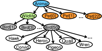
(a) AP’s tree

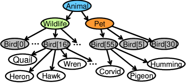
(b) RAP’s tree

Figure 4: trees induced by AP(a) and RAP(b). The numbers in brackets just indicate the index numbers of the exemplar nodes of their clusters. Non-exemplar nodes are collapsed to one of these exemplars. The nodes without number are those that cluster all nodes with the same name together.

The trees learned by both methods are shown in Figure 4. AP clusters both wild and domestic ‘bird’ nodes together in cluster number $50$ as illustrated in Figure 4(a), while, RAP separates them into two different clusters: cluster number $16$ (wild bird) and cluster number $55$ (domestic bird). By taking structural constraints into account, RAP is able to separate ‘bird’ into different senses. Specifically, during the inference process this constraint prevents all bird nodes from being clustered together, because this will create paths to this cluster from two different parent clusters: ‘wildlife’ and ‘pet’. The only valid configuration then is to have two ‘bird’ clusters: one under ‘wildlife’ and one under ‘pet’. The inference process optimizes the tree within this valid configuration. AP, on the other hand, does not have this machinery and, consequently, merges all ‘bird’ nodes together without concern for where the incoming links come from. The final correction step does not optimize the tree structure, and the tree learned by AP is worse than one learned by RAP.

Validation on Real-Wold Data

We also compared RAP against AP on the data collected from Flickr (?). We manually selected $15$ seed terms, and for each term used the following heuristic to obtain “relevant” saplings. First, we selected saplings whose root names were similar to the seed term. We then used the leaf node names of these saplings to select other saplings whose root names were similar to these names, and so on, for the total of two iterations. We used the settings described above but with the number of iterations limited to $2000$.

For each seed, we ran AP and RAP on all extracted saplings; then measured the net similarity of the induced tree. For measuring the induced tree’s structure in terms of bushiness and depth, we introduce a simple, yet intuitive measure, namely Area Under Tree(AUT), which takes both tree bushiness and depth into account. To calculate AUT for a given tree, we plot the distribution of the number of nodes at each level and then compute the area under the plot. Intuitively, trees that keep branching out at each level will get a larger AUT than those that short and thin. Suppose that we have a tree in which the number of nodes at $1^{st}$ and $2^{rd}$ level are $3$ and $4$, respectively. With the scale of tree depth set to $1.0$, AUT of this tree would be $0.5\times(1+3)+0.5\times(3+4)=5.5$.

	Entire Set		Induced Seed Trees
	Net Sim		# Trees		Best Tree’s Net Sim		Best Tree’s AUT
	AP	RAP	AP	RAP	AP	RAP	AP	RAP
africa	46.93	103.92	2	2	25.41	63.31	55	103
animal	3609.32	3839.88	4	4	142.48	156.28	606	727
asia	474.06	617.15	2	2	143.75	219.86	445.5	523.5
australia	167.65	227.24	2	2	72.11	123.41	104	151
bird	231.73	365.02	3	3	31.11	33.31	75	71.5
canada	278.7	312.29	2	2	46.32	50.62	127	138
craft	235.65	285.75	6	6	24.31	24.41	72.5	67.5
fish	124.83	132.43	1	1	44.61	45.71	69	68.5
insect	244.69	257.19	31	31	34.81	37.1	66.5	63
invertebrate	34.01	56.2	1	1	32.91	55.11	97.5	99.5
mammal	97.86	117.25	2	2	50.71	36.71	58.5	65
plant	565.72	714.7	2	2	12.3	13.4	19.5	19
sport	725.81	758.2	9	9	92.85	105.74	269	252.5
uk	640.48	754.16	1	1	370.84	526.7	633	673.5
usa	286.28	390.56	1	1	244.29	341.99	354.5	370

Table 1: The table presents the performance comparisons between AP and RAP by the net similarity for the entire data and the best induced tree (with highest net similarity) on $15$ different seed sets. The number of induced trees and Area Under Tree (AUT) are also reported.

Both quantitative and manual inspections confirm the advantages of RAP over AP. As shown in Table 1, RAP yields better net similarity in all cases. Although both approaches return the same number of trees, RAP appears to better cluster similar nodes in all but one case, namely ‘mammal’. In terms of AUT, though many trees are of similar quality, in cases where significant differences exist, they are in RAP’s favor. Manual inspection reveals that AP tends to “shatter” trees into isolated singletons rather than merge similar nodes together, as RAP does.

Related Work

Affinity propagation has been applied to many clustering problems, e.g. segmentation in computer vision (?). It provides a natural way to incorporate constraints while simultaneously improving the net similarity of the cluster assignments, which is not trivial to handle in standard clustering techniques. In addition, no strong assumption is required on the threshold, which determines whether clusters should be merged or not. Moreover, the cluster assignments can be changed during the inference process as suggested by the emergence of exemplars. Nevertheless, to our knowledge, there is no extension of AP algorithm to learn tree structures from many sparse and shallow trees as presented in this work.

There are many other SRL approaches that are applicable as well. For example, Markov Logic Networks (MLN) (?), a generic framework for solving probabilistic inference problems, may also be applied to folksonomy learning, by translating similarity function as well as constraints into predicates. Since our similarity function is continuous, hybrid MLN (HMLN) (?) would be required. The AP framework has advantages due to its simplicity; however we plan to investigate more comparative work with existing SRL approaches, especially as we explore more complex similarity functions.

Discussion and Conclusion

In this paper, we introduce relational affinity propagation (RAP), an extension to affinity propagation to learn structures from data by incorporating structural constraints. RAP optimizes the net similarity and it uses the structural constraint to find good solutions within a space of “valid” solutions. Thus, the final net similarity of the tree learned by RAP is better than AP. Our validations on toy and real-world data support this claim. For the future work, we would like to apply more sophisticated similarity function, which utilizes class labels as in a collective relational clustering approach in order to improve the quality of the learned structures. In addition, the structural constraints can be modified to guide RAP to induce other classes of graphs, e.g., a DAG. We would also like to extend RAP to apply on other structure learning problems.

Acknowledgments: this material is based upon work supported by the National Science Foundation under Grant No.IIS-0812677.

References

- [Bishop 2006] Bishop, C. M. 2006. Pattern Recognition and Machine Learning. Springer-Verlag.
- [Euzenat and Shvaiko 2007] Euzenat, J., and Shvaiko, P. 2007. Ontology Matching. Springer-Verlag.
- [Frey and Dueck 2007] Frey, B. J., and Dueck, D. 2007. Clustering by passing messages between data points. Science 312:972 –976.
- [Givoni and Frey 2009] Givoni, I. E., and Frey, B. J. 2009. A binary variable model for affinity propagation. Neural Comput 21(6):1589–1600.
- [Golder and Huberman 2006] Golder, S. A., and Huberman, B. A. 2006. Usage patterns of collaborative tagging systems. J. Inf. Sci. 32(2):198–208.
- [Kschischang, Frey, and Loeliger 2001] Kschischang, F.; Frey, B. J.; and Loeliger, H.-A. 2001. Factor graphs and the sum-product algorithm. IEEE Transactions on Information Theory 47:498–519.
- [Lazic et al. 2009] Lazic, N.; Givoni, I.; Frey, B.; and Aarabi, P. 2009. Floss: Facility location for subspace segmentation. In Proceedings of the International Conference on Computer Vision.
- [Plangprasopchok and Lerman 2009] Plangprasopchok, A., and Lerman, K. 2009. Constructing folksonomies from user-specified relations on flickr. In Proceedings of the World Wide Web conference.
- [Richardson and Domingos 2006] Richardson, M., and Domingos, P. 2006. Markov logic networks. Mach. Learn. 62:107–136.
- [Wang and Domingos 2008] Wang, J., and Domingos, P. 2008. Hybrid markov logic networks. In Proceedings of Association for the Advancement of Artificial Intelligence.