Renormalization-group description of nonequilibrium critical short-time relaxation processes: a three-loop approximation

Abstract

The influence of nonequilibrium initial values of the order parameter on its evolution at a critical point is described using a renormalization group approach of the field theory. The dynamic critical exponent $\theta^{\prime}$ of the short time evolution of a system with an $n$-component order parameter is calculated within a dynamical dissipative model using the method of $\varepsilon$-expansion in a three-loop approximation. Numerical values of $\theta^{\prime}$ for three-dimensional systems are determined using the Padé-Borel method for the summation of asymptotic series.

I Introduction

This study is devoted to the influence of nonequilibrium initial states on the evolution of magnetization $m(t)$ of a ferromagnetic system at a critical point. As is known H-H , anomalous features in the phenomena of critical dynamics are determined primarily by the long-range correlation of long-lived fluctuations of some thermodynamic variables. In this context, subject of fundamental interest to study is the process of critical relaxation of a system from an initial nonequilibrium state – for example, that created at temperatures much higher than the critical temperature and, hence, characterized by a short correlation length – to a strongly correlated state at the critical point. Janssen et al. Janssen showed that the critical evolution of a system from the initial nonequilibrium state with a small magnetization $m_{0}=m(0)\ll 1$ displays a universal scaling behavior of $m(t)$ over a short time early stage of this process, which is characterized by an anomalous increase in magnetization with time according to a power law. The exponent characterizing this relaxation process was calculated H-H within a renormalization group approach using the method of $\varepsilon$-expansion in a two-loop approximation. Later, the nonequilibrium critical relaxation in a short time regime was studied within a three-dimensional Ising model using methods of computer simulation Zheng . The results confirmed theoretical predictions concerning the power character of evolution of the magnetization of ferromagnetic systems, but the value of an exponent of $\theta^{\prime}=0.108(2)$ determined from these simulations significantly deviated from the theoretical predictions of $\theta^{\prime}=0.130$ (obtained by direct substitution of the parameter $\varepsilon=1$ for three-dimensional systems) and $\theta^{\prime}=0.138$ (obtained using the Padé-Borel method for the summation of a very short series with respect to $\varepsilon=1$).

According to the scaling theory, a singular part of the Gibbs potential $\Phi_{\mathrm{sing}}(t,\tau,h,m_{0})$ determining the state of a system in the critical region is characterized by a generalized homogeneity with respect to the main thermodynamic variables:

$$\begin{split}&\Phi_{\mathrm{sing}}(t,\tau,h,m_{0})\\ =b\Phi_{\mathrm{sing}}&(b^{a_{t}}t,b^{a_{\tau}}\tau,b^{a_{h}}h,b^{a_{m}}m_{0}),\end{split}$$ (1)

where $t$ is time, $\tau$ is the reduced temperature, $h$ is the field, $m_{0}$ is the initial magnetization, $b$ is the scaling factor, and $a_{i}$ are the scaling exponents. As a result, the magnetization $m=-\delta\Phi/\delta h$ of the system at the critical point ($\tau=0$, $h=0$) is characterized by the following time dependence:

$$m(t,m_{0})=t^{-(a_{h}+1)/a_{t}}F_{m}(m_{0}t^{-a_{m}/a_{t}}).$$ (2)

Expanding the right-hand side of Eq. (2) into series with respect to the small parameter $m_{0}t^{-a_{m}/a_{t}}$, we obtain the following power relation:

$$m(t)\sim t^{-(a_{h}+a_{m}+1)/a_{t}}\sim t^{\theta^{\prime}}.$$ (3)

All $a_{i}$ except $a_{m}$ can be related to well-known critical exponents that describe behavior of the system without effects related to a nonequilibrium initial state. For this reason, Janssen et al.Janssen introduced a new independent dynamic critical exponent $\theta^{\prime}$. The renormalization-group description of the nonequilibrium critical behavior of the system showed that this exponent takes positive values and, for $t>t_{cr}\sim m(0)^{-1/(\theta^{\prime}+\beta/z\nu)}$, the initial regime (characterized by an increase in the magnetization $m(t)$) changes to a traditional regime of critical relaxation toward the equilibrium state. The stage of critical relaxation is characterized by a time dependence of the magnetization according to the power law $m\sim t^{-\beta/\nu z}$ (Fig. 1), where $\beta$ and $\nu$ are well-known static exponents determining the equilibrium critical behavior of the magnetization and the correlation length, and $z$ is a dynamic exponent characterizing the critical slowing down of relaxation in the system. It can be shown that, when the system evolves from the initial ordered state with $m_{0}=1$, the time dependence of magnetization at the critical point is from the very beginning determined by the power law as $m\sim t^{-\beta/\nu z}$.

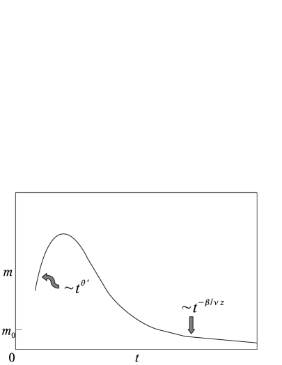
Figure 1: Schematic diagram of evolution of magnetization $m$ at a critical point, starting from an initial state with magnetization $m_{0}$.

II Description of the model

The critical behavior of a pure system in the equilibrium state is described using the Ginzburg–Landau–Wilson model Hamiltonian, which can be written as

$$\begin{split}H_{GL}[s]=&\int\!\mathrm{d}^{\mathrm{d}}x\,\Bigg{\{}\sum\limits_{\alpha=1}^{n}\frac{1}{2!}\left[\left(\nabla s_{\alpha}(\mathbf{x})\right)^{2}+\tau s_{\alpha}^{2}(\mathbf{x})\right]\\ &+\frac{g}{4!}\left(\sum\limits_{\alpha=1}^{n}s_{\alpha}^{2}(\mathbf{x})\right)^{2}\Bigg{\}},\end{split}$$ (4)

where $s(\mathbf{x})$ is the field of the $n$-component order parameter, $\tau$ is the reduced temperature of the second-order phase transition, and $g$ is the amplitude of interaction of order parameter fluctuations.

Let the realization of any configuration of the order parameter in the system at a given time $t$ be determined by the condition that the order parameter field $s(\mathbf{x},0)=s_{0}(\mathbf{x})$ at the initial instant $t=0$ (with the initial magnetization $m=m_{0}$) be characterized by the probability distribution $P[s_{0}]\sim\exp(-H_{0}[s_{0}])$, where

$$H_{0}[s_{0}]=\int\!\mathrm{d}^{\mathrm{d}}{x}\,\,\frac{\tau_{0}}{2}\left(s_{0}(\mathbf{x})-m_{0}(\mathbf{x})\right)^{2}.$$ (5)

In the most interesting case of pure relaxation dynamics of the order parameter (so-called Model A H-H ), the exponent $\theta^{\prime}$ is essentially new and cannot be expressed by means of the well-known static critical exponents and the parameters of equilibrium dynamics. The relaxation dynamics of the order parameter in this case is described by the Langevin equation

$$\partial_{t}s_{\alpha}(x,t)=-\lambda\frac{\delta H_{GL}[s]}{\delta s_{\alpha}}+\zeta_{\alpha}(x,t),$$ (6)

where $H_{GL}[s]$ is the Ginzburg–Landau–Wilson model Hamiltonian (4), $\lambda$ is the kinetic coefficient, and $\zeta(x,t)$ is the Gaussian random-noise source, which describes the influence of short-lived excitations. The randomnoise source is determined by the following probability functional:

$$P[\zeta]\sim\exp\left[-\frac{1}{4\lambda}\int d^{d}x\int dt(\zeta(x,t))^{2}\right];$$

$$\langle\zeta_{\alpha}(x,t)\rangle=0;$$ (7)

$$\langle\zeta_{\alpha}(x,t)\zeta_{\beta}(x^{\prime},t^{\prime})\rangle=2\lambda\,\delta_{\alpha\beta}\,\delta(x-x^{\prime})\delta(t-t^{\prime}).$$

Within the framework of the renormalization-group field theory, the critical dynamics Lawrie ; Bausch is described in terms of an auxiliary field $\tilde{s}(\mathbf{x})$ and a generating functional for the dynamic correlation functions and response functions. This functional is defined as follows:

$$\begin{split}W[h,\tilde{h}]&=\ln\Bigg{\{}\int\mathcal{D}(s,i\tilde{s})\exp\left(-\mathcal{L}[s,\tilde{s}]-H_{0}[s_{0}]\right)\\ &\times\exp\Biggl{(}\int\!\mathrm{d}^{\mathrm{d}}{x}\,\,\int\limits_{0}^{\infty}\!\mathrm{d}{t}\sum_{\alpha=1}^{n}(\tilde{h}_{\alpha}\tilde{s}_{\alpha}+h_{\alpha}s_{\alpha})\Biggr{)}\Bigg{\}},\end{split}$$ (8)

where $\mathcal{L}$ is the action functional expressed as

$$\begin{split}\mathcal{L}[s,\tilde{s}]&=\int\limits_{0}^{\infty}\!\mathrm{d}{t}\int\!\mathrm{d}^{\mathrm{d}}{x}\,\,\sum_{\alpha=1}^{n}\Biggl{\{}\tilde{s}_{\alpha}\Biggl{[}\dot{s}_{\alpha}+\lambda(\tau-\nabla^{2})s_{\alpha}\\ &+\frac{\lambda g}{6}s_{\alpha}\Bigl{(}\sum_{\beta=1}^{n}s_{\beta}^{2}\Bigr{)}-\lambda\tilde{s}_{\alpha}\Biggr{]}\Biggr{\}}.\end{split}$$ (9)

An analysis of the Gaussian component of functional (9) for $g=0$ allows the following expressions for the bare response function $G_{0}(p,t-t^{\prime})$ and the bare correlation function $C_{0}^{(D)}(p,t,t^{\prime})$ to be obtained for the Dirichlet boundary condition ($\tau_{0}=\infty$) Janssen :

$$G_{0}(p,t-t^{\prime}) = \exp[-\lambda(p^{2}+\tau)|t-t^{\prime}|],$$ (10)

$$C_{0}^{(D)}(p,t,t^{\prime}) = C_{0}^{(e)}(p,t-t^{\prime})+C_{0}^{(i)}(p,t+t^{\prime}),$$ (11)

where

$$C_{0}^{(e)}(p,t-t^{\prime}) = \frac{1}{p^{2}+\tau}\,e^{-\lambda(p^{2}+\tau)|t-t^{\prime}|},$$ (12)

$$C_{0}^{(i)}(p,t+t^{\prime}) = -\frac{1}{p^{2}+\tau}\,e^{-\lambda(p^{2}+\tau)(t+t^{\prime})}.$$ (13)

III Renormalization-group analysis of the model

In the renormalization-group analysis of the model with allowance for the interaction of critical fluctuations in the order parameter, singularities appearing in the dynamic correlation functions and response functions in the limit as $\tau\to 0$ were eliminated using the procedure of dimensional regularization and the scheme of minimum substraction Vasiliev followed by reparametrization of the Hamiltonian parameters and by multiplicative field renormalization in functional (8) as follows:

$$\begin{array}[]{ll}s\to Z_{s}^{1/2}s,&\tilde{s}\to Z_{\tilde{s}}^{1/2}\tilde{s},\\ \lambda\to\left(Z_{s}/Z_{\tilde{s}}\right)^{1/2}\lambda,&\tau\to Z_{s}^{-1}Z_{\tau}\mu^{2}\tau,\\ g\to Z_{g}Z_{s}^{-2}\mu^{\varepsilon}g,&\tilde{s}_{0}\to\left(Z_{\tilde{s}}Z_{0}\right)^{1/2}\tilde{s}_{0},\end{array}$$ (14)

where $\varepsilon=4-d$, and $\mu$ is a dimensional parameter. Calculation of all renormalization constants $Z_{i}$ (except for $Z_{0}$) was described in Lawrie . A scheme for the calculation of $Z_{0}$ and the results of calculations in a two-loop approximation were presented in Janssen . In this study, $Z_{0}$ was calculated in the subsequent three-loop approximation of the renormalization-group field theory.

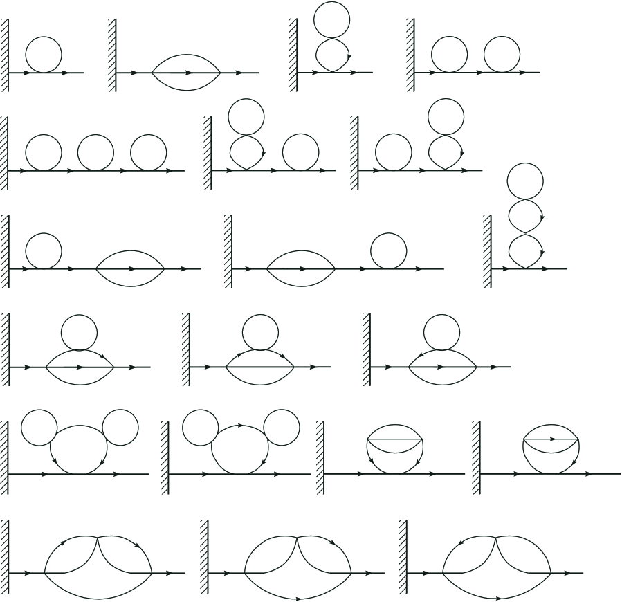
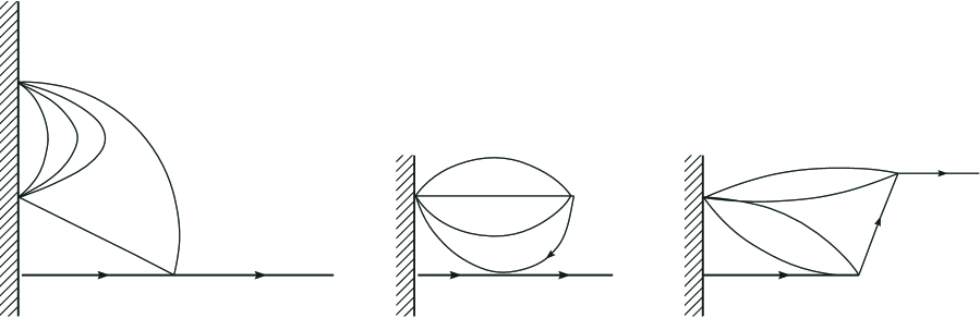
Figure 2: Diagrams determining contributions to the vertex functions $\Gamma_{1,0}^{(i)}$. Curves without and with arrows correspond to the bare correlators and the bare response functions, respectively. The vertical line corresponds to the surface $t=0$.

Figure 3: Diagrams determining contributions to the vertex functions $\Gamma_{1,0}^{(\mathrm{eq})}$.

Introduction of the initial conditions of type (5) into the theory makes it necessary renormalize the response function $\langle s(p,t)\tilde{s}_{0}(-p,0)\rangle$, which determines the influence of the initial state of the system on its relaxation dynamics. The correction terms in the self-energy part of the response function appear due to the interaction of fluctuations of the order parameter and are characterized by reducible dynamic Feynman diagrams, since they are calculated using correlator (11), which does not possess the property of translational invariance with respect to time. Janssen et al. Janssen introduced the following representation for this response function:

$$\begin{split}G_{1,1}^{(i)}(p,t)&=\langle s(p,t)\tilde{s}_{0}(-p,0)\rangle\\ &=\int\limits_{0}^{t}\!\mathrm{d}t^{\prime}\,\bar{G}_{1,1}(p,t,t^{\prime})\,\Gamma_{1,0}^{(i)}(p,t^{\prime})_{[\tilde{s}_{0}]}.\end{split}$$ (15)

In a three-loop approximation, the one-particle vertex function $\Gamma_{1,0}^{(i)}(p,t)_{[\tilde{s}_{0}]}$ with a single field insertion $\tilde{s}_{0}$ is described by the diagrams presented in Fig. 3, which obey the requirement of containing at least a single $C_{0}^{(i)}$ correlator. The factor $\bar{G}_{1,1}(p,t,t^{\prime})$ is determined by the equilibrium component of the correlator $C_{0}^{(e)}$ in Eq. (11). It should be noted that this correlator differs from the equilibrium response function $G_{1,1}^{(eq)}(p,t-t^{\prime})$ because the integration in (15) with respect to time is performed starting from $t=0$ instead of $t=-\infty$. However, it is possible to establish a functional relationship Oerding between these functions by using the functional $H_{GL}[s_{0}]$ (4) instead of (5) with a new interaction vertex in action functional (9):

$$\frac{\lambda g}{6}\int\!dt\int\!d^{d}x\sum_{\alpha,\beta=1}^{n}\left(\tilde{s}_{0\alpha}s_{0\alpha}\right)\left(s_{0\beta}\right)^{2}.$$ (16)

The additional vertex function $\Gamma_{1,0}^{(eq)}$, which is localized on the surface $t=0$, appears due to averaging over the initial fields. By analogy with representation (15), we also obtain

$$G_{1,1}^{(eq)}(p,t-t^{\prime})=\int_{t^{\prime}}^{t}dt^{\prime\prime}\bar{G}_{1,1}(p,t,t^{\prime\prime})\Gamma^{(eq)}_{1,0}(p,t^{\prime\prime})_{[\tilde{s}(t^{\prime})]}.$$ (17)

Solving the integral equation

$$\delta(t-t^{\prime})=\int_{t^{\prime}}^{t}dt^{\prime\prime}K(q,t^{\prime\prime},t^{\prime})\Gamma^{(eq)}_{1,0}(q,t)_{[\tilde{s}(t^{\prime\prime})]}$$ (18)

in each order of the theory, we obtain the kernel $K(q,t^{\prime\prime},t^{\prime})$. Note that fluctuation corrections to this kernel in the model under consideration appear only in the third order (Fig. 3). Using Eqs. (15) and (17), performing renormalization of the fields according to Eq. (14), and obeying the requirement of eliminating poles with respect to $\varepsilon$ in each order of the theory so that the renormalization constant $Z_{0}$ would remain finite in the limit as $\varepsilon\to 0$, we eventually obtain the following expression for this constant:

$$Z_{0}^{-1/2}\int\limits_{0}^{\infty}dte^{-i\omega t}\hat{\Gamma}_{1,0}(q=0,t)_{[\tilde{s}_{0}]},$$ (19)

Upon sequential realization of the procedure described above and calculation of the diagrams using the method of $\varepsilon$-expansion, the renormalization constant in the three-loop approximation is as follows:

$$Z_{0}=1+\frac{n+2}{6}\frac{g}{\varepsilon}+\frac{n+2}{12}\left[\frac{n+5}{3}+\varepsilon\left(\ln 2-\frac{1}{2}\right)\right]\\ \times\left(\frac{g}{\varepsilon}\right)^{2}+\frac{n+2}{216}\Biggl{[}(n+5)(n+6)\\ +\Bigg{(}\frac{1}{6}(-19+9\ln 2)(n+2)+\frac{1}{3}(-7+6\ln 2)(n+8)\Bigg{)}\varepsilon{}\\ -1.18679(n+3.13882)\varepsilon^{2}\Biggr{]}\left(\frac{g}{\varepsilon}\right)^{3}.$$ (20)

The invariance with respect to the renormalizationgroup transformations of the generalized connected Green’s function

$$G^{\tilde{M}}_{N,\tilde{N}}\equiv\langle[s]^{N}[\tilde{s}]^{\tilde{N}}[\tilde{s}_{0}]^{\tilde{M}}\rangle$$

can be expressed in terms of the renormalization-group Callan–Symanzik differential equation Janssen ; Vasiliev :

$$\begin{split}\Bigg{\{}\mu\partial_{\mu}+&\zeta\lambda\partial_{\lambda}+\kappa\tau\partial_{\tau}+\beta\partial_{g}+\frac{N}{2}\gamma+\frac{\tilde{N}}{2}\tilde{\gamma}\\ +&\frac{\tilde{M}}{2}(\tilde{\gamma}+\gamma_{0})+\zeta\tau_{0}^{-1}\partial_{\tau_{0}^{-1}}\Bigg{\}}G_{N,\tilde{N}}^{\tilde{M}}=0.\end{split}$$ (21)

The renormalization-group functions representing the coefficients in Eq. (21) are given by the following expressions:

$$\zeta \equiv(\mu\partial_{\mu})_{0}\ln\lambda=\dfrac{1}{2}(\tilde{\gamma}-\gamma), \kappa \equiv(\mu\partial_{\mu})_{0}\ln\tau,$$

$$\gamma_{0} \equiv(\mu\partial_{\mu})_{0}\ln Z_{0}, \gamma \equiv(\mu\partial_{\mu})_{0}\ln Z_{s},$$ (22)

$$\tilde{\gamma} \equiv(\mu\partial_{\mu})_{0}\ln Z_{\tilde{s}}, \beta \equiv(\mu\partial_{\mu})_{0}g,$$

where $(\partial_{\mu})_{0}\equiv\left(\frac{\partial}{\partial\mu}\right)_{0}$ denotes differentiation with constant initial parameters $g$, $\lambda$ and $\tau$. For a short time regime of nonequilibrium critical relaxation, the only essentially new quantity is the renormalization-group function $\gamma_{0}$. In the three-loop approximation used in this study, this function is expressed as follows:

$$\begin{split}\gamma_{0}=&-\frac{n+2}{6}g\Biggl{(}1+\left(\ln 2-\frac{1}{2}\right)g\\ &-0.0988989\left(n+3.13882\right)g^{2}\Biggr{)}+O(g^{4}).\end{split}$$ (23)

The fixed point $g^{*}$ of the renormalization-group transformation is determined from the equation $\beta(g^{*})=0$. The general solution of differential Eq. (21) by the method of characteristics at the fixed point has the following scaling form Janssen

$$G^{\tilde{M}}_{N,\tilde{N}}(\{x,t\},\tau,\tau^{-1}_{0},\lambda,g^{*},\mu)=l^{(d-2+\eta_{s})\frac{N}{2}}$$

$$\times l^{(d+2+\eta_{\tilde{s}})\frac{\tilde{N}}{2}+(d+2+\eta_{\tilde{s}}+\eta_{0})\frac{\tilde{M}}{2}}$$ (24)

$$\times G^{\tilde{M}}_{N,\tilde{N}}(\{lx,l^{2+\zeta^{*}}t\},\tau l^{-2+\kappa^{*}},\tau^{-1}_{0}l^{2+\zeta^{*}},\lambda,g^{*},\mu),$$

where $\eta_{s}=\gamma^{*}$, $\eta_{\tilde{s}}=\tilde{\gamma^{*}}$ and $\eta_{0}=\gamma_{0}^{*}$ – are the exponents of anomalous dimensions. The functions entering into Eq. (III) can be related to the critical exponents involved in the scaling relations, for example:

$$z =2+\zeta^{*},\qquad 1/\nu=2-\kappa^{*},$$ (25)

$$\theta^{\prime} =-\left(\zeta^{*}+\gamma^{*}+\frac{\gamma_{0}^{*}}{2}\right)\left/(2+\zeta^{*})\right.,$$

which determine the critical relaxation dynamics ($z$), correlation length ($\nu$), and nonequilibrium evolution ($\theta^{\prime}$) of the magnetization. In determining the и value, we used the data of Kleinert et al. Kleinert on the coordinate of the stable fixed point $g^{*}$ and the results of calculations Antonov of the dynamic critical exponent $z$ for the Ising model, which refined (in the three-loop approximation) the previous values of exponents for this model. The final expression for the dynamic critical exponent

$$\begin{split}z=2+\frac{\varepsilon^{2}}{2}\left(6\ln\frac{4}{3}-1\right)\frac{n+2}{(n+8)^{2}}\\ \times\left[1+\varepsilon\left(\frac{6(3n+14)}{(n+8)^{2}}-0.4384812\right)\right],\end{split}$$ (26)

represents a generalization of the previous results Antonov to the case of systems with $n$-component order parameters. The final expression for the critical exponent $\theta^{\prime}$ is as follows:

$$\theta^{\prime} =\frac{(n+2)}{4(n+8)}\,\varepsilon\Bigg{(}1+\frac{6\varepsilon}{(n+8)^{2}}\left(n+3+(n+8)\ln\frac{3}{2}\right)-$$

$$-\frac{7.2985}{(n+8)^{4}}\,\varepsilon^{2}\Big{(}n^{3}+17.3118n^{2}+153.2670n$$ (27)

$$+383.5519\Big{)}\Bigg{)}+O(\varepsilon^{4}).$$

IV Analysis of results. Conclusions

The series of $\varepsilon$-expansions exhibit factorial divergence, but they can be considered in an asymptotic context Wilson . In order to obtain physically reasonable values of the critical exponents for three-dimensional systems at $\varepsilon=1$, special methods for the summation of asymptotic series have been developed Baker ; LeGuillou ; Antonenko ; Kazakov ; Suslov ; Prudnikov , the most effective being the Padé-Borel, Padé-Borel-Leroy, and conformal mapping techniques. We used the Padé-Borel method to perform the asymptotic summation of $\varepsilon$-expansion series (III) for the critical exponent $\theta^{\prime}$. According to this method, the series

$$\theta^{\prime}(\varepsilon)=\sum\limits_{n=1}^{\infty}c_{n}\varepsilon^{n}$$ (28)

is replaced by the integral

$$\begin{split}\theta^{\prime}(\varepsilon)&=\int\limits_{0}^{\infty}e^{-t}B(\varepsilon t)dt,\\ B(x)&=\sum\limits_{n=1}^{\infty}B_{n}x^{n},\qquad B_{n}=\frac{c_{n}}{n!}.\end{split}$$ (29)

where $B(x)$ is the so-called Borel image. In contrast to the initial series (28) having a zero radius of convergence, the Borel image has a finite radius of convergence determined by the parameters of the asymptotic nth term of series (29) for $n\gg 1$. Then, the Borel image is subjected to the Padé approximation, according to which $B(x)$ is replaced by a rational function of the following type:

$$[L/M]=\frac{\sum\limits_{i=0}^{L}a_{i}x^{i}}{\sum\limits_{j=0}^{M}b_{j}x^{j}}\qquad(M\geq 1),$$ (30)

the expansion of which into Taylor’s series (in the vicinity of $x=0$) coincides with that of the Borel image as far as possible. The function of type (30) has $L+1$ coefficients in the numerator and $M+1$ coefficients in the denominator. The entire set of coefficients is determined to within a constant factor (for certainty, $b_{0}=1$), so that there are a total of $L+M+1$ free parameters. This implies that, in the general case, the coefficients of expansion of the $[L/M]$ function into Taylor’s series must coincide with the corresponding coefficients of series (28). If this series has a finite number $N$ of terms, the number of coefficients in expansion of the $[L/M]$ function must obey the condition $L+M\leq N$.

In the case of a three-term series under consideration, the summation of the $\varepsilon$-expansion for exponent $\theta^{\prime}$ was performed in the $[2/1]$ approximation. In the given order of the theory, the choice of this approximation is (in accordance with the results of analysis performed in Prudnikov ) preferred for obtaining more accurate value of the sum. The results of calculations are presented in the Table 1.

Table 1: Results of calculations of the critical exponent $\theta^{\prime}$ for the Ising model and XY model in comparison to the results of computer simulations

	Critical exponent $\theta^{\prime}$
Calculation method	Ising model	XY-model
Two-loop approximation
Substitution $\varepsilon=1$	$0.130$	$0.154$
Padé–Borel summation	0.138	0.170
Three-loop approximation
Substitution $\varepsilon=1$	$0.0791$	$0.0983$
Padé–Borel summation	0.1078(22)	0.1289(23)
Computer simulation	0.108(2) Zheng	0.144(10)Kolesnikov

A comparison of the results of our calculations of the critical exponent и to the values obtained by numerical modeling within the Ising model Zheng and XY model Kolesnikov using the method of short time dynamics (see Table 1) clearly demonstrates that the values obtained in the three-loop approximation better with the results of computer simulations as compared to the results of a two-loop approximation.

In this study, we have presented a field theory description of the nonequilibrium critical relaxation of a system within the most interesting dynamical model A (according to the Hohenberg–Halperin classification H-H ). It is shown that only beginning with a three-loop approximation does the theory of these processes involve an additional vertex function $\Gamma_{1,0}^{(eq)}$ localized on the surface of initial states ($t=0$), which provides fluctuation corrections to the dynamic response function due to the influence of nonequilibrium initial states. As a result, only allowance for these fluctuation corrections (reflecting the influence of the nonequilibrium initial states) ensures adequate description of the relaxation process. Using this three-loop approximation and the method of $\varepsilon$-expansion, it is possible to obtain the values of independent dynamic critical exponent $\theta^{\prime}$ describing the evolution of the system during a short time evolution in close agreement with the results of computer simulations.

- (1) P.C. Hohenberg and B.I. Halperin, Rev.Mod.Phys. 49, 435 (1977).
- (2) H.K. Janssen, B. Schaub, and B. Schmittmann, Z. Phys. 73, 539 (1989).
- (3) A. Jaster, J. Mainville, L. Schulke, and B. Zheng, J.Phys.A: Math.Gen. 32, 1395 (1999).
- (4) I.D. Lawrie and V.V. Prudnikov, J.Phys. C. 17, 1655 (1984).
- (5) R. Bausch, H.K. Janssen, and H. Wagner, Z. Phys. 24, 113 (1976).
- (6) A.N. Vasil’ev, The Field Theoretic Renormalization Group in Critical Behavior Theory and Stochastic Dynamics (St. Petersburg Institute of Nuclear Physics, Russian Academy of Sciences, St. Petersburg, 1998; Chapman and Hall, New York, 2004).
- (7) K. Oerding and H.K. Janssen, J.Phys.A: Math.Gen. 26, 3369 (1993).
- (8) H. Kleinert, J. Neu, U. Schulte-Frohlinde, K.G. Chetyrkin et al., Phys.Lett. B 272, 39 (1991).
- (9) N.V. Antonov and A.N. Vasil’ev, Teor. Mat. Fiz. 60, 59 (1984).
- (10) C. De Dominicis, J.Physique (France) 37, Suppl.1, C1-247 (1976).
- (11) K. Wilson and J. Kogut, The Renormalization Group and the -Expansion (Wiley, New York, 1974; Mir, Moscow, 1975).
- (12) G.A. Baker, B.G. Nickel, M.S. Green et al., Phys. Rev. Lett. 36, 1351 (1976); Phys. Rev. B 17, 1365 (1978).
- (13) J.C. Le Guillou, J.Zinn-Justin, Phys. Rev. Lett. 39, 95 (1977); Phys. Rev. B 21, 3976 (1980).
- (14) S.A. Antonenko, A.I. Sokolov, Phys. Rev. B 51, 1894 (1995).
- (15) D.I. Kazakov, O.V. Tarasov, and D.V. Shirkov, Teor. Mat. Fiz. 38, 15 (1979); D.I. Kazakov and V.S. Popov, Zh.Éksp. Teor. Fiz. 122 (4), 675 (2002) [JETP 95 (4),581 (2002)].
- (16) I. M. Suslov, Zh. Éksp. Teor. Fiz. 120 (1), 5 (2001) [JETP 93 (1), 1 (2001)].
- (17) A.S. Krinitsyn, V.V. Prudnikov, and P.V. Prudnikov, Teor. Mat. Fiz. 147, 137 (2006).
- (18) E.A. Gergertd, V.Yu. Kolesnikov, V.V. Prudnikov, and P.V. Prudnikov, Vestn. Omsk. Gos. Univ., No. 4, 28 (2007).