A Method for Measuring the Bias
of High-Redshift Galaxies from Cosmic Variance

Abstract

As deeper observations discover increasingly distant galaxies, characterizing the properties of high-redshift galaxy populations will become increasingly challenging and paramount. We present a method for measuring the clustering bias of high-redshift galaxies from the field-to-field scatter in their number densities induced by cosmic variance. Multiple widely-separated fields are observed to provide a large number of statistically-independent samples of the high-redshift galaxy population. The expected Poisson uncertainty is removed from the measured dispersion in the distribution of galaxy number counts observed across these many fields, leaving, on average, only the contribution to the scatter expected from cosmic variance. With knowledge of the $\Lambda$-Cold Dark Matter power spectrum, the galaxy bias is then calculated from the measured cosmic variance. The results of cosmological N-body simulations can then be used to estimate the halo mass associated with the measured bias. We use Monte Carlo simulations to demonstrate that Hubble Space Telescope pure parallel programs will be able to determine galaxy bias at $z\gtrsim 6$ using this method, complementing future measurements from correlation functions.

1. Introduction

Galaxy bias, the spatial clustering strength of galaxies relative to the matter field, encodes important information about the connection between the luminous baryons of galaxies and the dark matter (DM) halos that host them. The galaxy bias $b$, defined as the ratio between the galaxy and matter correlation functions (CFs) $b^{2}\equiv\xi_{gg}/\xi_{mm}$, reflects both the clustering of galaxy-scale DM halos and how luminous galaxies populate halos of a given mass. A self-consistent connection between the luminosity function (LF), angular CF, and mass-to-light ratio of galaxies can be developed (e.g., van den Bosch et al., 2003; Vale & Ostriker, 2004; Conroy et al., 2006; Lee et al., 2009).

CF estimates of bias, which require large samples of galaxies spanning a wide range of angular separations, are remarkably successful at low-redshift (e.g., Norberg et al., 2001; Zehavi et al., 2002). Angular CF measurements on smaller samples have been performed for Lyman Break Galaxies (LBGs) (Giavalisco et al., 1998; Arnouts et al., 1999; Ouchi et al., 2004, 2005; Foucaud et al., 2003; Hamana et al., 2004; Adelberger et al., 2005; Allen et al., 2005; Kashikawa et al., 2006; Lee et al., 2006, 2009) and Lyman-$\alpha$ emitters (Ouchi et al., 2003; Hamana et al., 2004; Kovač et al., 2007; Gawiser et al., 2007) over a range of redshifts. These studies have extended high-significance $(>3\sigma)$ detections of bias out to $z\sim 5$.

At the highest redshifts ($z\gtrsim 5.5$), limited samples have made significant detections of galaxy bias difficult. McLure et al. (2009) used a $0.63$deg² area observed by the UKIRT Infrared Deep Sky Survey Ultra Deep Survey and the Subaru XMM-Newton Survey to measure the clustering of $5<z<6$ LBGs with $z<26$AB ($b=5.2_{-0.8}^{+1.2}$), but most of their systems lie at redshifts $z<5.5$. Overzier et al. (2006) reported a measurement of bias for $i$-dropout galaxies in Great Observatories Origins Deep Survey (GOODS) ($b=4.1_{-2.6}^{+1.5}$) but no detection of clustering in the Ultra Deep Field. A study of $z$-dropout galaxies in the Subaru Deep Field and GOODS-N by Ouchi et al. (2009) indicated that $z\sim 7$ galaxies may be strongly clustered, but measuring bias from only 22 candidates is challenging.

Given the difficulty of measuring clustering of high-redshift galaxies from the angular CF, an exploration of complementary approaches is warranted. As a salient example, Adelberger et al. (1998) used a counts-in-cells analysis (Peebles, 1980) to measure the clustering of redshift $z\sim 3$ LBGs from statistical fluctuations in their number densities. Having obtained spectroscopic redshifts for $N\sim 270$ LBGs in six fields, they split their samples into redshift slices and calculated the variance in galaxy counts in rectangular volumes. The bias was then measured from the excess dispersion in the number counts beyond the Poisson variance.

In this Letter, we present calculations that demonstrate the bias of high-redshift ($z\gtrsim 6$) galaxies can also be measured from field-to-field dispersion in galaxy counts from photometric dropout samples. Specifically, we use Monte Carlo simulations to demonstrate that pure parallel programs with the Hubble Space Telescope (HST) that obtain large numbers ($\gtrsim 100$) of statistically-independent samples of $z\approx 6-7$ galaxies with the Advanced Camera for Surveys (ACS) or Wide Field Camera 3 (WFC3) (e.g., Ratnatunga, 2002; Sparks, 2002; Trenti, 2008; Yan, 2008) can provide a significant measurement of high-redshift galaxy bias. Throughout, we adopt the cosmological parameter values determined by the $5$-year Wilkinson Microwave Anisotropy Probe joint analysis (Komatsu et al., 2009).

2. Measuring Halo Bias from Cosmic Variance

Consider a number $N_{\mathrm{fields}}$ of telescope pointings on the sky. At the location $\mathbf{x}_{i}$ of the $i$-th field the expected number density of galaxies is

$$n(\mathbf{x}_{i})=\bar{n}[1+b\delta_{\mathrm{DM}}(\mathbf{x}_{i})],$$ (1)

where $\bar{n}$ is the mean average galaxy number density, $b$ is the bias, and $\delta_{\mathrm{DM}}\equiv(\rho-\bar{\rho})/\bar{\rho})$ is the matter overdensity of the field. The matter variance $\langle{\delta_{\mathrm{DM}}^{2}}\rangle$, averaged over many survey volumes $V$, is

$$\sigma_{\mathrm{DM}}^{2}(V,z)\equiv\langle{\delta_{\mathrm{DM}}^{2}}\rangle=D^{2}(z)\int\frac{d^{3}k}{(2\pi)^{3}}P(k)|\hat{W}(\mathbf{k},V)|^{2}$$ (2)

where $D(z)$ is the growth factor at redshift $z$, $P(k)$ is the matter power spectrum (we use the Eisenstein & Hu 1998 transfer function), and

$$\hat{W}(\mathbf{k},V)=\mathrm{sinc}\left(\frac{k_{x}r\Theta_{x}}{2}\right)\mathrm{sinc}\left(\frac{k_{y}r\Theta_{y}}{2}\right)\mathrm{sinc}\left(\frac{k_{z}\delta r}{2}\right)$$ (3)

is the Fourier transform of the rectangular volume $V=r\Theta_{x}\times r\Theta_{y}\times\delta r$ with angular area $\Theta_{x}\times\Theta_{y}$ and depth $\delta r$ at distance $r$. The expected dispersion in galaxy counts owing to cosmic variance is simply $\sigma_{\mathrm{g}}^{2}=b^{2}\sigma_{\mathrm{DM}}^{2}$ (e.g., Stark et al., 2007; Trenti & Stiavelli, 2008; Muñoz et al., 2010; Robertson, 2010).

With a sample of $N_{\mathrm{fields}}$ fields, the distribution of galaxy counts $N$, with mean $\bar{N}$ per field, will have a dispersion $\sigma_{\mathrm{N}}^{2}\equiv\langle{(N-\bar{N})^{2}}\rangle\approx\sigma_{\mathrm{g}}^{2}\bar{N}^{2}+\bar{N}$ that includes contributions from both cosmic and Poisson variance. The bias can be estimated as

$$b^{2}\approx\frac{\sigma_{\mathrm{N}}^{2}-\bar{N}}{\bar{N}^{2}\sigma_{\mathrm{DM}}^{2}}.$$ (4)

Below, we demonstrate that this estimate can be used to measure the bias of high-redshift galaxies from multiple widely-separated HST pointings. The accuracy of this method will depend on $N_{\mathrm{fields}}$ and the relative size of the cosmic and Poisson variances, and we now explore these effects through Monte Carlo simulations.

3. Monte Carlo Simulations of Galaxy Bias Measurements from Cosmic Variance

To simulate high-redshift galaxy number counts, we require a model for the distribution of galaxy counts for each field in our sample. Below, we describe our model distribution and our Monte Carlo realizations of this distribution that act as our model observational samples.

The initial cosmological linear overdensity field is a Gaussian random field with dispersion $\sigma_{\mathrm{DM}}^{2}$ given by Equation 2. As the density field evolves owing to gravitation, the overdensity distribution changes to maintain the positivity condition on the density ($\delta_{\mathrm{DM}}\geq-1$). The shape of the quasi-linear overdensity distribution can be approximated by a lognormal (Coles & Jones, 1991; Kofman et al., 1994). The corresponding galaxy overdensity distribution will be lognormal, written as

$$p_{\mathrm{LN}}(\delta_{\mathrm{g}}|\sigma_{\mathrm{g}}^{2})=\frac{1}{\sqrt{2\pi x^{2}}}\exp\left[-\frac{1}{2}\left(\frac{y}{x}+\frac{x}{2}\right)^{2}\right],$$ (5)

where $y=(1+\delta_{\mathrm{g}})$ and $x=(1+\sigma_{\mathrm{g}}^{2})^{1/2}$. The expected cosmic variance is $\sigma_{\mathrm{g}}<1$ (see below), so the quasi-linear distribution is appropriate.

At each location $\mathbf{x}_{i}$, the number of galaxies observed will be a Poisson-sampled random variate of Equation 5. The probability of observing $N$ galaxies in fields of volume $V$ with cosmic variance $\sigma_{\mathrm{g}}^{2}$, given the expected number $\bar{N}=\bar{n}V$, is

$$p(N|\bar{N},\sigma_{\mathrm{g}}^{2})=\frac{1}{N!}\int_{-1}^{\infty}\mathrm{d}\delta_{\mathrm{g}}p_{\mathrm{LN}}(\delta_{\mathrm{g}}|\sigma_{\mathrm{g}}^{2})[(1+\delta_{\mathrm{g}})\bar{N}]^{N}e^{-(1+\delta_{\mathrm{g}})\bar{N}}$$ (6)

(Adelberger et al., 1998). Our simulations of the bias measurement consist of drawing discrete random samples from this distribution, as described below.

3.1. Observational Model

Measuring the bias from the dispersion in galaxy counts requires an observational program suited to probing many high-redshift galaxy samples. Our presented method is motivated by HST programs (Programs 9488, PI Ratnatunga, 9575 and 9584, PI Sparks, 11700, PI Trenti, and 11702, PI Yan) that use pure parallel observations with ACS or WFC3 to probe $z\gtrsim 6-7$ galaxy populations. While the total numbers of long-duration and multiple-passband observations in the HST archive are few ($\sim 10s$), we expect that similar pure parallel observations will be obtained by HST in ongoing and future cycles. We will therefore model future HST pure parallel programs that obtain ACS $i$- and $z$-band data, which would allow for $i$-dropout selection at $z\sim 6$ to $z\sim 26.5$AB (single orbit exposure, extrapolated from Beckwith et al., 2006). Additionally, as an example comparison with WFC3 observations, we will model the Yan WFC3 program that can select $\mathrm{F600LP}-\mathrm{F098M}$ dropouts at $6.5\lesssim z\lesssim 7.3$, and reach $\mathrm{F098M}\sim 27$AB magnitude sensitivity (single orbit exposure), but our method can be adapted for use with any WFC3 filter strategy. We adopt these survey designs, summarized in Table 1, as our points of comparison for modeling observational measurements of high-redshift galaxy bias.

We wish to simulate the number of high-redshift galaxies these pure parallel surveys will discover in each field. The mean abundance $\bar{N}$ per field is determined by integrating a Schechter (1976) LF over the volume probed by each pointing. For modeling the ACS observations of $i$-dropouts at $5.5\leq z\leq 6.5$, we adopt the measured $z\sim 6$ LF parameters $\phi_{\star}=0.0014~{}\mathrm{Mpc}^{-3}\mathrm{mag}^{-1}$, $M_{\star}=-20.24$AB, and $\alpha=-1.74$ (Bouwens et al., 2007). With these values, we expect $\bar{N}=4.3$ per $11.3$ arcmin² ACS field in the magnitude range $M_{\mathrm{UV}}\lesssim-20.5$. To approximate the conversion between $z_{\mathrm{AB}}$ apparent and restframe $M_{\mathrm{UV}}$ used by Bouwens et al. (2006), we use $M_{\mathrm{UV}}-z_{\mathrm{AB}}\approx-47$.

For modeling the WFC3 observations the $z\sim 7$ LF is uncertain at $6.5\leq z\leq 7.3$, but if we adopt the measured $z\sim 7$ LF parameters $\phi_{\star}=0.0014~{}\mathrm{Mpc}^{-3}\mathrm{mag}^{-1}$, $M_{\star}=-19.91$AB, and $\alpha=-1.77$ (Oesch et al., 2010), we expect $\bar{N}=1.04$ per $4.7$ arcmin² WFC3 field in the UV absolute magnitude range $M_{\mathrm{UV}}\lesssim-20.2$. Our results will be similar for other estimates of the $z\sim 7$ LF (e.g., McLure et al., 2010; Yan et al., 2009).

Galaxy counts for each field can be generated by discretely sampling the Equation 6, with a variance $\sigma_{\mathrm{g}}$ and bias $b$ determined using the abundance-matching methodology presented in Robertson (2010). This method assumes the galaxies occupy DM halos with an abundance and bias appropriate for their high redshifts (Tinker et al., 2008, 2010).

Table 1Model Parallel Surveys

Redshift	Detector	Orbits/Field	Depth	$\phi_{\star}$	$M_{\star}$	$\alpha$	$\bar{N}$	$\sigma_{\mathrm{g}}$	$1/\sqrt{\bar{N}}$	Fields/$SNR\sim 3$
			[AB mag]	[Mpc-3 mag-1]	[AB mag]
$5.5\leq z\leq 6.5$	ACS	4	$z\sim 26.5$	$1.4\times 10^{-3}\,$	-20.24	-1.74	4.29	0.37	0.48	40
$6.5\leq z\leq 7.3$	WFC3	4	$Y\sim 27$	$1.4\times 10^{-3}\,$	-19.91	-1.77	1.04	0.50	0.98	130

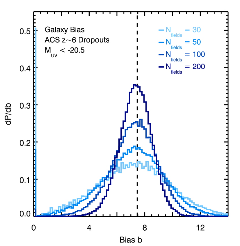
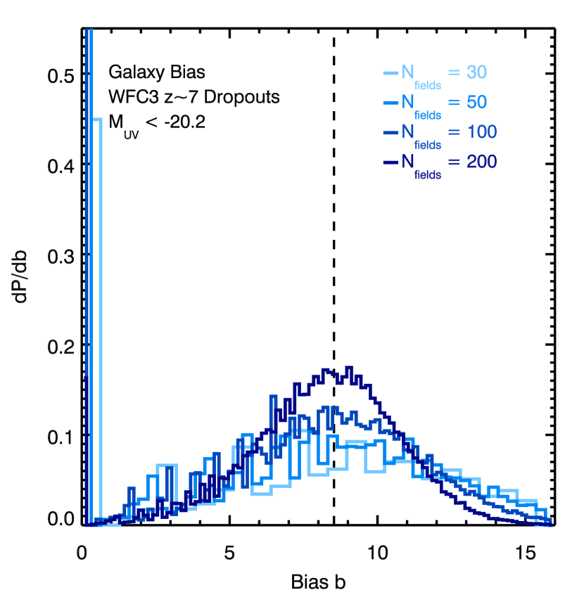
Figure 1.— Monte Carlo simulations of galaxy bias measurements from the field-to-field variation in number counts across $N=30-200$ (light to dark blue) statistically-independent, widely-separated fields. Shown are 100,000 realizations of the measurement for $z\sim 6$ ACS $i$-band (left panel) and $z\sim 7$ WFC3 $\mathrm{F600LP}$-band (right panel) dropouts with UV absolute magnitudes $M_{\mathrm{UV}}\lesssim-20.5$AB and $M_{\mathrm{UV}}\lesssim-20.2$AB, respectively. As the number of independent fields increases, the $SNR$ of the cosmic variance measurement increases rapidly. For some realizations the scatter in the distribution of number counts is smaller than Poisson and cosmic variance cannot be measured ($b=0$ bins, for a discussion see §3.2).

3.2. Uncorrelated ACS Fields

The left panel of Figure 1 shows $N_{\mathrm{reals}}=100,000$ realizations of the galaxy bias measurement for $z\sim 6$ galaxies with $M_{\mathrm{UV}}\lesssim-20.5$AB across $N_{\mathrm{fields}}=30-200$ (light to dark blue) widely-separated ACS fields. For this example magnitude range at redshifts $5.5\leq z\leq 6.5$, the mean number of galaxies per 11.3 arcmin² is $\bar{N}=4.3$ and $\sigma_{\mathrm{DM}}\approx 0.05$. The model bias calculated for this galaxy abundance is $b\approx 7.5$ (vertical dashed line). The mean galaxy count per ACS field $\bar{N}$ and the sample variance $\sigma_{\mathrm{N}}^{2}$ are calculated from each realization. The “observed” bias is then estimated using Equation 4, histogrammed, and normalized such that the area under each curve is unity.

For each $N_{\mathrm{fields}}$-sized sample the mean expected measured bias is accurate, with $\Delta_{b}\equiv(\langle{b}\rangle-b)/b\approx-0.025$ for $N_{\mathrm{fields}}=30$ decreasing to $\Delta_{b}\approx-0.014$ for $N_{\mathrm{fields}}=200$. The expected uncertainty $\sigma_{b}$ in the measured bias decreases from $\sigma_{b}/b\approx 0.36$ for $N_{\mathrm{fields}}=30$ to $\sigma_{b}/b\approx 0.16$ for $N_{\mathrm{fields}}=200$, improving as $\propto 1/\sqrt{N_{\mathrm{fields}}}$. When $N_{\mathrm{fields}}$ is small, the measured dispersion $\sigma_{\mathrm{N}}^{2}$ can be less than $\bar{N}$, providing $b^{2}<0$ in Equation 4. Such catastrophic failures happen infrequently for ACS $i$-dropout samples ($<7.5\%$ for $N_{\mathrm{fields}}=30$ and $<0.3\%$ for $N_{\mathrm{fields}}=100$, shown as the $b=0$ bin).

Given these results, we suggest that using the dispersion in galaxy counts determined from ACS photometric samples in uncorrelated fields to measure bias will be a novel method for learning about the spatial clustering of $z\sim 6$ galaxies. The bias measurement significance increases from $SNR\approx 3$ with $N_{\mathrm{fields}}=40$ to $SNR\approx 6.4$ with $N_{\mathrm{fields}}=200$ fields for $i$-dropouts with magnitudes near $M_{\star}$, providing a method for measuring bias that increases in sensitivity with an increasing number of independent samples.

3.3. Uncorrelated WFC3 Fields

The right panel of Figure 1 shows $N_{\mathrm{reals}}=100,000$ realizations of the bias measurement for $z\sim 7$ galaxies with absolute magnitudes $M_{\mathrm{UV}}\lesssim-20.2$AB across $N_{\mathrm{fields}}=30-200$ (light to dark blue) widely-separated WFC3 fields. For this magnitude range at redshifts $6.5\leq z\leq 7.3$, the expected mean number of galaxies per 4.7 arcmin² is $\bar{N}=1.04$ and $\sigma_{\mathrm{DM}}\approx 0.06$. The model bias calculated for this galaxy abundance is $b\approx 8.5$ (vertical dashed line). The observed mean galaxy count per WFC3 field $\bar{N}$ and the sample variance $\sigma_{\mathrm{N}}^{2}$ are calculated from each of the $N_{\mathrm{reals}}$ realizations. The “observed” bias is then estimated using Equation 4, histogrammed, and normalized such that the area under each curve is unity.

These histograms demonstrate that characterizing the bias of rare $z\sim 7$ galaxies will be challenging. Approximately $N_{\mathrm{fields}}=130$ pointings are needed to measure the bias of these galaxies with an appreciable signal-to-noise ($SNR\sim 3$) in an accurate way ($\Delta_{b}\lesssim-0.023$). With fewer fields ($N_{\mathrm{fields}}\leq 100$), the expected uncertainty in the measured bias is large ($\sigma_{b}/b\geq 0.36$) and overestimated ($\Delta_{b}\gtrsim 0.05$). When $N_{\mathrm{fields}}$ is small, the measured dispersion $\sigma_{\mathrm{N}}^{2}$ can be less than $\bar{N}$, providing $b^{2}<0$ in Equation 4. In these catastrophic failures ($26\%$ for $N_{\mathrm{fields}}=30$ and $9\%$ for $N_{\mathrm{fields}}=100$, shown as the $b=0$ bin), an unusually small Poisson scatter limits sensitivity to the cosmic variance in number counts. These failures decrease as the number of pointings increases (to $3\%$ for $N_{\mathrm{fields}}=200$).

The larger numbers of $z\sim 6$ galaxies per ACS field compared with the number of $z\sim 7$ galaxies per WFC3 field (see §3.2) makes the $z\sim 6$ ACS experiment much easier. While $N_{\mathrm{fields}}\sim 130$ pointings are required to significantly ($SNR\sim 3$) measure the bias, such a determination would provide a crucial constraint on the nature of $z\sim 7$ galaxies. Current HST programs may have too few fields to perform this experiment, but extensions or new pure parallel programs will likely provide enough pointings in the next few HST cycles to successfully measure the bias of $z\sim 7$ from cosmic variance.

3.4. Correlated Fields

Pure parallel observations with ACS and WFC3 provide a novel method to obtain statistically-independent samples of the high-redshift galaxy population. However, the forthcoming HST Multi-Cycle Treasury (MCT) programs will probe greater numbers of contiguous pointings. While the MCT areas may be used to measure the angular correlation function of high-redshift galaxies, one may wonder whether contiguous areas may be used to measure bias from cosmic variance. Here, we estimate the effects of correlations in the galaxy counts induced by large-scale density modes shared between nearby pointings. We consider $z\sim 6$ dropouts in ACS pointings, as the improved statistics relative to $z\sim 7$ dropouts more clearly illustrate the effects of field-to-field correlations.

The detailed correlation between nearby fields will depend on the geometry of the tiling and the separation between fields, and are difficult to calculate for general survey designs. However, we estimate the field-to-field correlations in a contiguous tiling as follows (for another estimate, see Hu & Cohn, 2006).

Consider as before $N_{\mathrm{fields}}$ pointings, but arranged in a contiguous tiling. The cosmic variance of an independent field with volume $V$ will depend on $\sigma_{\mathrm{g}}^{2}(V,z)$. Correspondingly, the galaxy counts in the larger volume $N_{\mathrm{fields}}V$ will have a sample variance $\sigma_{\mathrm{g}}^{2}(N_{\mathrm{fields}}V,z)$. The number counts within the $i$-th field of the $N_{\mathrm{fields}}$ pointings within the contiguous survey will then be correlated with the other $j$ fields approximately at the level of

$$\rho\equiv\frac{\sigma_{ij}^{2}}{\sigma_{ii}\sigma_{jj}}\approx\frac{\sigma_{\mathrm{g}}^{2}(N_{\mathrm{fields}}V,z)}{\sigma_{\mathrm{g}}^{2}(V,z)}.$$ (7)

This typically underestimates the correlation between very nearby or adjacent fields, but should approximate the average correlation of the most widely-spaced pointings within the contiguous area. The matrix describing the correlation between fields $i$ and $j$ then has a simple form, with the diagonal elements $\Sigma_{ii}=1$ and off-diagonal elements $\Sigma_{i,j\neq i}=\rho$.

To model the counts in correlated fields, we use a standard Cholesky decomposition technique to instill the distribution of galaxy overdensities with the correlation matrix $\Sigma$, and then Poisson-sample the correlated distribution to generate the counts in each field. Figure 2 shows the results of this procedure. Since the number counts in fields are correlated ($\rho\approx 0.3$ for $N_{\mathrm{fields}}=30$ and $\rho\approx 0.09$ for $N_{\mathrm{fields}}=200$), the dispersion $\sigma_{\mathrm{N}}^{2}$ in the ACS galaxy counts becomes smaller than in the uncorrelated case. The resulting estimates for the cosmic variance are correspondingly smaller, leading to a bias measurement that is underestimated ($\Delta_{b}=-0.15$ for $N_{\mathrm{fields}}=30$ and $\Delta_{b}=-0.06$ for $N_{\mathrm{fields}}=200$) and is more susceptible to catastrophic (measured $b\leq 0$) failures ($13.6\%$ for $N_{\mathrm{fields}}=30$).

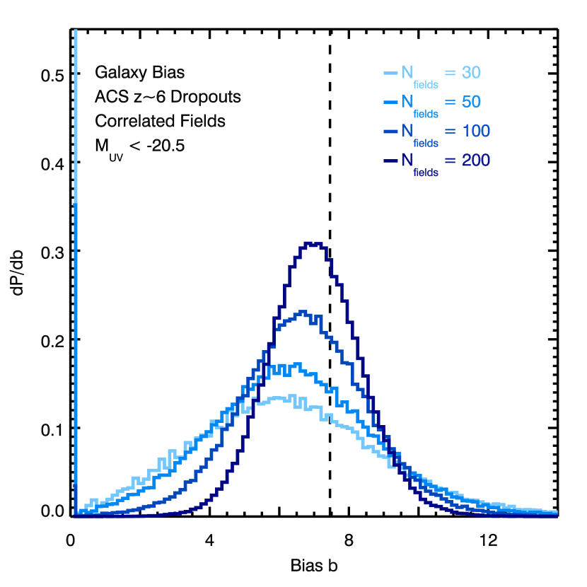
Figure 2.— Same as left panel of Figure 1, but for a contiguous survey where large scale structure correlates the number counts in each field. The field-to-field correlations decrease the dispersion in galaxy counts, and leads to a 10-20% underestimate of the galaxy bias.

3.5. Estimating Halo Masses from Galaxy Bias

The simulations presented in §3.2 and 3.3 demonstrate that the bias of high-redshift galaxies can be measured directly from the variance in number counts between uncorrelated fields. Using the connection between bias and DM halo mass calculated from cosmological simulations (Tinker et al., 2008, 2010), the galaxy bias can be used to estimate the characteristic mass of DM halos with similar spatial clustering strength. For detailed discussions of the connection between halo mass and bias, we refer the reader to Robertson (2010) and Tinker et al. (2010).

Figure 3 shows the characteristic halo mass estimated by converting the bias (Figure 1) using the Tinker et al. (2010) bias-mass relation determined from cosmological simulations. For the case of $M_{\mathrm{UV}}\lesssim-20.5$AB magnitude $i$-dropout galaxies at redshift $z\sim 6$ with bias $b\approx 7.5$, the mass of halos with the same bias at $z\sim 6$ is $M_{\mathrm{halo}}\approx 2.1\times 10^{11}h^{-1}M_{\sun}$ (dashed line). The bias can provide a precise estimate of a characteristic DM halo mass ($8\%$ in $\log M$ for $N_{\mathrm{fields}}=30$ and $3\%$ in $\log M$ for $N_{\mathrm{fields}}=200$) that, while skewed, is accurate ($\Delta_{M}\equiv[\langle{\log M}\rangle-\log M]/\log M=-0.03$ for $N_{\mathrm{fields}}=30$ and $\Delta_{M}=-0.007$ for $N_{\mathrm{fields}}=200$). This measure of a characteristic halo mass only corresponds to the halo mass of $i$-dropout galaxies if each halo hosts one galaxy and mass strongly correlates with luminosity (see Robertson, 2010), but provides a convenient conceptual tool for discussing the approximate mass scale of high-redshift galaxies.

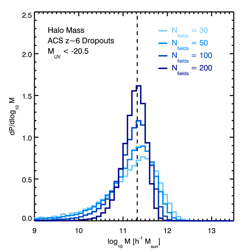
Figure 3.— Characteristic halo mass inferred from the bias of $z\sim 6$ ACS $i$-band dropouts with UV absolute magnitudes $M_{\mathrm{UV}}\lesssim-20.5$AB. The bias is measured from number count variations across $N=30-200$ (light to dark blue) fields (see left panel of Fig 1), and then converted into a mass using the Tinker et al. (2010) bias function for DM halos.

4. Summary and Discussion

We have presented a simple counts-in-cells method (e.g., Peebles, 1980; Adelberger et al., 1998) for measuring the bias of high-redshift galaxies from the field-to-field variation in number counts induced by cosmic variance. The number of high-redshift galaxies of a given luminosity are measured in a large number independent, widely-separated fields. The Poisson contribution to the variance in the number counts across these fields is removed, leaving a cosmic variance contribution that depends on the bias and the mean matter overdensity fluctuations on the scale of the survey field volume. We use Monte Carlo simulations of the bias measurement to estimate the effectiveness of the method for example galaxy populations, $i$-dropouts at $z\sim 6$ in ACS-sized fields and $\mathrm{F600LP}$-dropouts at $z\sim 7$ in WFC3-sized fields. Our method can be adapted for other dropout filter strategies. At $z\sim 6$ ($z\sim 7$) the method should provide a measurement of galaxy bias with $SNR\gtrsim 3$ for luminosities near $M_{\mathrm{UV}}\approx M_{\star}$ when $N_{\mathrm{fields}}\geq 40$ ($N_{\mathrm{fields}}\gtrsim 130$) fields are used. The uncertainty on the galaxy bias improves with an increasing number of independent fields as $\approx 1/\sqrt{N_{\mathrm{fields}}}$. These requirements on the number of fields are concomitant with the expected number of pointings available from extensions to ongoing pure parallel HST programs (Trenti, 2008; Yan, 2008), and the potential for using this method to measure high-redshift galaxy bias is therefore promising. We also show that using correlated, nearby fields to perform the presented measurement typically leads to an underestimate of the bias owing to a correlation-induced decrease in the dispersion of galaxy number counts.

The measured bias can be associated with a characteristic mass of DM halos with similar clustering. We show that the typical uncertainty in the bias measured using the presented method corresponds to an uncertainty in the inferred DM halo mass of $\sim$ a few percent in $\log M$ for $i$-dropouts. Combining these estimates of halo mass with the observed luminosities allow for an estimate of a mass-to-light ratio, which can constrain the connection between the galaxies’ observed LF and their clustering (Yang et al., 2003; Conroy et al., 2006). Numerous effects can alter the correspondence between bias and halo mass, and we therefore view the presented method as primarily a measure of bias and interpret the halo mass estimates with caution. Our simulations assume that the high-redshift galaxy population is essentially volume limited and pure. Methods to handle incompleteness for LBG samples have already been engineered (e.g., Bouwens et al., 2008; Reddy & Steidel, 2009). Contamination at a fractional level of $f_{c}$ will lower the bias by an amount $\Delta_{b}\approx(1-f_{c})$ (e.g., Ouchi et al., 2004). Using simulations that include red $z\sim 2$ galaxy interlopers with $f_{c}=0.2$ and a bias of $b\approx 5.5$ (Quadri et al., 2007), we find that the measured bias at $z\sim 6$ is lowered by $\sim 17\%$. This systematic error is comparable to the statistical error on the bias when $N_{\mathrm{fields}}\gtrsim 200$. Lastly, not every parallel field will be useful for measuring high-redshift galaxy counts owing, e.g., to possible bright star or Galactic reddening contamination, and the efficiency of the presented method may be correspondingly decreased.

References

- Adelberger et al. (1998) Adelberger, K. L., Steidel, C. C., Giavalisco, M., Dickinson, M., Pettini, M., & Kellogg, M. 1998, ApJ, 505, 18
- Adelberger et al. (2005) Adelberger, K. L., Steidel, C. C., Pettini, M., Shapley, A. E., Reddy, N. A., & Erb, D. K. 2005, ApJ, 619, 697
- Allen et al. (2005) Allen, P. D., Moustakas, L. A., Dalton, G., MacDonald, E., Blake, C., Clewley, L., Heymans, C., & Wegner, G. 2005, MNRAS, 360, 1244
- Arnouts et al. (1999) Arnouts, S., Cristiani, S., Moscardini, L., Matarrese, S., Lucchin, F., Fontana, A., & Giallongo, E. 1999, MNRAS, 310, 540
- Beckwith et al. (2006) Beckwith, S. V. W., et al. 2006, AJ, 132, 1729
- Bouwens et al. (2006) Bouwens, R. J., Illingworth, G. D., Blakeslee, J. P., & Franx, M. 2006, ApJ, 653, 53
- Bouwens et al. (2007) Bouwens, R. J., Illingworth, G. D., Franx, M., & Ford, H. 2007, ApJ, 670, 928
- Bouwens et al. (2008) —. 2008, ApJ, 686, 230
- Coles & Jones (1991) Coles, P., & Jones, B. 1991, MNRAS, 248, 1
- Conroy et al. (2006) Conroy, C., Wechsler, R. H., & Kravtsov, A. V. 2006, ApJ, 647, 201
- Eisenstein & Hu (1998) Eisenstein, D. J., & Hu, W. 1998, ApJ, 496, 605
- Foucaud et al. (2003) Foucaud, S., McCracken, H. J., Le Fèvre, O., Arnouts, S., Brodwin, M., Lilly, S. J., Crampton, D., & Mellier, Y. 2003, A&A, 409, 835
- Gawiser et al. (2007) Gawiser, E., et al. 2007, ApJ, 671, 278
- Giavalisco et al. (1998) Giavalisco, M., Steidel, C. C., Adelberger, K. L., Dickinson, M. E., Pettini, M., & Kellogg, M. 1998, ApJ, 503, 543
- Hamana et al. (2004) Hamana, T., Ouchi, M., Shimasaku, K., Kayo, I., & Suto, Y. 2004, MNRAS, 347, 813
- Hu & Cohn (2006) Hu, W., & Cohn, J. D. 2006, Phys. Rev. D, 73, 067301
- Kashikawa et al. (2006) Kashikawa, N., et al. 2006, ApJ, 637, 631
- Kofman et al. (1994) Kofman, L., Bertschinger, E., Gelb, J. M., Nusser, A., & Dekel, A. 1994, ApJ, 420, 44
- Komatsu et al. (2009) Komatsu, E., et al. 2009, ApJS, 180, 330
- Kovač et al. (2007) Kovač, K., Somerville, R. S., Rhoads, J. E., Malhotra, S., & Wang, J. 2007, ApJ, 668, 15
- Lee et al. (2009) Lee, K., Giavalisco, M., Conroy, C., Wechsler, R. H., Ferguson, H. C., Somerville, R. S., Dickinson, M. E., & Urry, C. M. 2009, ApJ, 695, 368
- Lee et al. (2006) Lee, K., Giavalisco, M., Gnedin, O. Y., Somerville, R. S., Ferguson, H. C., Dickinson, M., & Ouchi, M. 2006, ApJ, 642, 63
- McLure et al. (2009) McLure, R. J., Cirasuolo, M., Dunlop, J. S., Foucaud, S., & Almaini, O. 2009, MNRAS, 395, 2196
- McLure et al. (2010) McLure, R. J., Dunlop, J. S., Cirasuolo, M., Koekemoer, A. M., Sabbi, E., Stark, D. P., Targett, T. A., & Ellis, R. S. 2010, MNRAS, 403, 960
- Muñoz et al. (2010) Muñoz, J. A., Trac, H., & Loeb, A. 2010, MNRAS, 623
- Norberg et al. (2001) Norberg, P., et al. 2001, MNRAS, 328, 64
- Oesch et al. (2010) Oesch, P. A., et al. 2010, ApJ, 709, L16
- Ouchi et al. (2005) Ouchi, M., et al. 2005, ApJ, 635, L117
- Ouchi et al. (2009) —. 2009, ApJ, 706, 1136
- Ouchi et al. (2003) —. 2003, ApJ, 582, 60
- Ouchi et al. (2004) —. 2004, ApJ, 611, 685
- Overzier et al. (2006) Overzier, R. A., Bouwens, R. J., Illingworth, G. D., & Franx, M. 2006, ApJ, 648, L5
- Peebles (1980) Peebles, P. J. E. 1980, The large-scale structure of the universe. (Princeton University Press)
- Quadri et al. (2007) Quadri, R., et al. 2007, ApJ, 654, 138
- Ratnatunga (2002) Ratnatunga, K. 2002, in HST Proposal, 9488–+
- Reddy & Steidel (2009) Reddy, N. A., & Steidel, C. C. 2009, ApJ, 692, 778
- Robertson (2010) Robertson, B. E. 2010, ApJ, 713, 1266
- Schechter (1976) Schechter, P. 1976, ApJ, 203, 297
- Sparks (2002) Sparks, W. 2002, in HST Proposal, 9575–+
- Stark et al. (2007) Stark, D. P., Loeb, A., & Ellis, R. S. 2007, ApJ, 668, 627
- Tinker et al. (2008) Tinker, J., Kravtsov, A. V., Klypin, A., Abazajian, K., Warren, M., Yepes, G., Gottlöber, S., & Holz, D. E. 2008, ApJ, 688, 709
- Tinker et al. (2010) Tinker, J. L., Robertson, B. E., Kravtsov, A. V., Klypin, A., Warren, M. S., Yepes, G., & Gottlober, S. 2010, arXiv:1001.3162
- Trenti (2008) Trenti, M. 2008, in HST Proposal, 11700–+
- Trenti & Stiavelli (2008) Trenti, M., & Stiavelli, M. 2008, ApJ, 676, 767
- Vale & Ostriker (2004) Vale, A., & Ostriker, J. P. 2004, MNRAS, 353, 189
- van den Bosch et al. (2003) van den Bosch, F. C., Yang, X., & Mo, H. J. 2003, MNRAS, 340, 771
- Yan (2008) Yan, H. 2008, in HST Proposal, 11702–+
- Yan et al. (2009) Yan, H., Windhorst, R., Hathi, N., Cohen, S., Ryan, R., O’Connell, R., & McCarthy, P. 2009, arXiv:0910.0077
- Yang et al. (2003) Yang, X., Mo, H. J., & van den Bosch, F. C. 2003, MNRAS, 339, 1057
- Zehavi et al. (2002) Zehavi, I., et al. 2002, ApJ, 571, 172