Part I 0

B. DASGUPTA² Email:brahmananda.dasgupta@uah.edu    DASTGEER SHAIKH^1,2 Email:dastgeer.shaikh@uah.edu    P. K. SHUKLA^{3 1}Department of Physics and
²Center for Space Physics and Aeronomic Research (CSPAR),
University of Alabama at Huntsville, Huntsville, AL 35805. USA.
³Institut für Theoretische Physik IV, Fakultät für Physik und Astronomie, Ruhr-Universität Bochum, D-44780 Bochum, Germany

I–LABEL:lastpage

Dispersive magnetized waves in the solar wind plasma

B. DASGUPTA² Email:brahmananda.dasgupta@uah.edu    DASTGEER SHAIKH^1,2 Email:dastgeer.shaikh@uah.edu    P. K. SHUKLA^{3 1}Department of Physics and
²Center for Space Physics and Aeronomic Research (CSPAR),
University of Alabama at Huntsville, Huntsville, AL 35805. USA.
³Institut für Theoretische Physik IV, Fakultät für Physik und Astronomie, Ruhr-Universität Bochum, D-44780 Bochum, Germany

Abstract

We derive a generalized linear dispersion relation of waves in a strongly magnetized, compressible, homogeneous and isotropic quasineutral plasma. Starting from a two fluid model, describing distinguishable electron and ion fluids, we obtain a six order linear dispersion relation of magnetized waves that contains effects due to electron and ion inertia, finite plasma beta and angular dependence of phase speed. We investigate propagation characteristics of these magnetized waves in a regime where scale lengths are comparable with electron and ion inertial length scales. This regime corresponds essentially to the solar wind plasma where length scales, comparable with ion cyclotron frequency, lead to dispersive effects. These scales in conjunction with linear waves present a great deal of challenges in understanding the high frequency, small scale dynamics of turbulent fluctuations in the solar wind plasma.

1 Introduction

Solar wind plasma is an admixture of waves, structures, and turbulent fluctuations that comprises multitude of length and time scales. Owing to a great deal of disparity in the time and spatial scales, solar wind plasma exhibits rich and complex dynamical evolution. Since the solar wind plasma is strongly magnetized, the presence of waves and their consequent interactions with fluctuations complicate our understanding of many aspects. For instance, the solar wind fluctuations yield a composite spectrum [[1]] as described in the schematic of figure 1. This spectrum describes the power spectral density (PSD) as a function of frequency and can be divided into five distinct regions. The frequencies smaller than $10^{5}$ Hz, namely region I, lead to a PSD that has a spectral slope of ­1 [[1, 2]]. The region II extends from $10^{5}$ Hz to or less than ion/proton gyrofrequency where the spectral slope exhibits an index of ­3/2 or ­5/3. The latter, a somewhat controversial issue, is characterized essentially by fully developed turbulence. The region II connects to the region III by means of a spectral break at length­scales corresponding to ion inertial length­scales and frequencies corresponding to ion gyrofrequencies. The onset of the spectral break is disputed. This regime is often referred to as dissipative regime which exhibits a PSD with a much broader spectral slope that varies between ­2 and ­5 [[6, 3, 4]]. Notably, the dynamics of the length­scales in this region cannot be described by the usual compressible or incompressible MHD models that possess characteristic frequencies smaller than ion gyro frequencies. A two fluid MHD model needs to be invoked to examine the dynamics of these high frequency and fast time scale processes. What is notable in these spectra is the waves in different regimes that interact with the turbulent fluctuations and influence the cascade dynamics [[16, 17, 18]]. Despite their prominent existence in different regimes, less is understood about the evolution of these waves and their dynamical role in governing the turbulent spectrum. For example, it is argued that the spectral break results from the damping of ion cyclotron waves. The latter is contrasted by Shaikh & Zank [[5]] who report that Hall forces could play a critical role in producing the spectral break. Similarly, the excitation and interaction of whistler waves in high frequency turbulence has been disputed recently [[7, 8, 9, 10]]. Motivated by these issues, we in this paper investigate linear waves in strongly magnetized plasma that are relevant to the understanding of the solar wind turbulence spectra depicted in Fig 1. Our main objective here is to develop a comprehensive understanding of the propagating linear waves in strongly magnetized plasma especially in the regimes III, IV and V of Fig 1. We further concentrate on a high beta plasma, because the solar wind plasma fluctuations are characterized typically by a high beta plasma beyond 1 AU (astronomical unit).

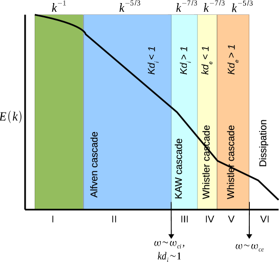
Figure 1: Schematic of the solar wind composite spectrum as a function of frequency (wavenumber). Magnetized waves play a critical role in the transition from region II (MHD regime) to region III (kinetic or Hall MHD regime). The onset of regions III and IV is associated with high frequency whistler waves where electron and ion motions are decoupled. Regions IV and V are identified as whistler wave cascade regimes.

In section 2, we describe our two fluid model that contains all possible modes in the magnetized solar wind plasma. A generalized linear dispersion relation is derived. In section 3, we describe various possible roots, corresponding to modes. This section also describes the solution of the generalized dispersion relation and focuses on waves especially associated with a high beta (pressure and magnetic energy ratio) plasma. Section 4 deals with the effect of plasma beta on the propagation characteristics of dispersive waves. Finally, a summary is presented in section 5.

2 Linear Dispersion Relation for two fluid plasma with finite electron mass

We start with a two-fluid model (ion with suffix $i$ and electron with suffix $e$). Using usual notations and with finite electron mass, i.e., $m_{e}\neq 0$, the ion and electron continuity equations, momentum equations, energy equations together with the Maxwell’s equation (neglecting displacement current) are written as (in CGS Gaussian unit)

$$\frac{\partial n_{i}}{\partial t}+\nabla\cdot(n_{i}{\bf u_{i}})=0,\quad\frac{\partial n_{e}}{\partial t}+\nabla\cdot(n_{e}{\bf u_{e}})=0,$$ (1)

$$m_{i}n_{i}\left(\frac{\partial{\bf u_{i}}}{\partial t}+{\bf u_{i}}\cdot\nabla{\bf u_{i}}\right) = -\nabla p_{i}+n_{i}e\left({\bf E}+\frac{1}{c}{\bf u_{i}}\times{\bf B}\right),$$ (2)

$$m_{e}n_{e}\left(\frac{\partial{\bf u_{e}}}{\partial t}+{\bf u_{e}}\cdot\nabla{\bf u_{e}}\right) = -\nabla p_{e}-n_{e}e\left({\bf E}+\frac{1}{c}{\bf u_{e}}\times{\bf B}\right),$$ (3)

$$\frac{\partial p_{i}}{\partial t}+{\bf u_{i}}\cdot\nabla p_{i}+\gamma_{i}p_{i}\nabla\cdot{\bf u_{i}}=0,\quad\frac{\partial p_{e}}{\partial t}+{\bf u_{e}}\cdot\nabla p_{e}+\gamma_{e}p_{e}\nabla\cdot{\bf u_{e}}=0,$$ (4)

$$\nabla\times{\bf B} = \frac{4\pi e}{c}(n_{i}{\bf u_{i}}-n_{e}{\bf u_{e}}),$$ (5)

$$\frac{\partial{\bf B}}{\partial t} = -c\nabla\times{\bf E},$$ (6)

$$\nabla\cdot{\bf B} = 0,$$ (7)

where $n_{i},n_{e}$ are the ion and electron number densities, $m_{i},m_{e}$ are the ion and electron mass, ${\bf u_{i}},{\bf u_{e}}$ are the ion and electron velocity, $p_{i},p_{e}$ are the ion and electron pressure,$\gamma_{i},\gamma_{e}$ are ratio of the specific heats for ions and electrons,respectively, and E is the electric field and B is the magnetic field. We use the linearized forms of the above equations with the following perturbation scheme for any variable $\psi_{\alpha}=\psi_{\alpha 0}+\tilde{\psi}_{\alpha},~{}~{}(\alpha=i,e$):

$$n_{\alpha}=n_{\alpha 0}+\tilde{n}_{\alpha};\quad p_{\alpha}=p_{\alpha 0}+\tilde{p}_{\alpha};\quad{\bf u}={\bf\tilde{u}}_{\alpha};\quad{\bf B}={\bf B_{0}}+{\bf{\tilde{B}}}~{}~{}~{}{\bf E}={\bf\tilde{E}};$$ (8)

with $n_{\alpha 0},p_{\alpha 0},B_{0}$ are constant and uniform in space. We assume the space-time dependence of a perturbed variable $\psi(x,y,z,t)$ as, $\tilde{\psi}\sim\exp[i({\bf k}\cdot{\bf r}-\omega t)]$. Further, we introduce the plasma displacement vector $\xi_{\alpha}$ as, ${\bf\tilde{u}}_{\alpha}=\partial{\bf\xi_{\alpha}}/\partial t=-i\omega\xi_{\alpha}$, with $\xi_{\alpha}$ as a vector. From the linearized equations for ion and electron continuity equations, and the energy equations, one gets, (replacing  $\partial/\partial t\rightarrow-i\omega;\quad\nabla\rightarrow i{\bf k}$) the following:

$$\tilde{n}_{\alpha}=-in_{\alpha 0}({\bf k}\cdot\xi_{\alpha}),\quad\tilde{p}_{\alpha}=-i\gamma_{\alpha}p_{\alpha 0}({\bf k}\cdot\xi_{\alpha}),$$ (9)

The linearized form of (5) after combining with linearized form of (6), can be written as, (with $n_{i0}=n_{e0}=n_{0}$),

$${\bf k}\times{\bf k}\times{\bf\tilde{E}}=-\omega^{2}\frac{4\pi n_{0}e}{c^{2}}({\bf\xi_{i}}-{\bf\xi_{e}})$$ (10)

Finally, we write the linearized forms of momentum conservation equations as:

$$-\omega^{2}m_{i}n_{0}{\bf\xi_{i}} = -\gamma_{i}p_{i0}{\bf k}({\bf k}\cdot{\bf\xi_{i}})+n_{0}e\left({\bf\tilde{E}}-\frac{i\omega}{c}~{}{\bf\xi_{i}}\times{\bf B_{0}}\right),$$ (11)

$$-\omega^{2}m_{e}n_{0}{\bf\xi_{i}} = -\gamma_{e}p_{e0}{\bf k}({\bf k}\cdot{\bf\xi_{e}})+n_{0}ed_{e}^{2}~{}{\bf k}\times{\bf k}\times{\bf\tilde{E}}-n_{0}e\left({\bf\tilde{E}}-\frac{i\omega}{c}~{}{\bf\xi_{e}}\times{\bf B_{0}}\right),$$

where we used $n_{i0}=n_{e0}=n_{0}$ and replaced ${\bf\xi_{e}}$ the displacement vector for electron by the relation obtained from (10), i.e.,

$${\bf\xi_{e}}={\bf\xi_{i}}+\frac{c^{2}}{4\pi n_{0}e\omega^{2}}~{}{\bf k}\times{\bf k}\times{\bf\tilde{E}};$$

and introduced the electron inertial length $d_{e}=c/\omega_{pe}$,  $\omega_{pe}$ being the electron plasma frequency. From eqn. (10)taking a dot-product with k, and also using the continuity equation (9) we get

$${\bf k}\cdot{\bf\xi_{i}}={\bf k}\cdot{\bf\xi_{e}},\qquad\tilde{n}_{e}=\tilde{n}_{i},$$ (13)

where the second equation denotes the quasineutrality condition. Equations (11) and (2) are our starting equations for deriving the dispersion relation for a two fluid plasma. We followed the procedures adopted by Ishida et al., to get the dispersion relation and we omit the derivation in this work for brevity. We proceed by adding both the equations, eliminating the perturbed electric field ${\bf\tilde{E}}$ in terms of ${\bf\xi_{i}}$ using (11) and finally taking the dot product of the resulting equation for ${\bf\xi_{i}}$ with three independent vectors, ${\bf k},~{}{\bf{\hat{b}}}$ and ${\bf k}\times{\bf{\hat{b}}}$, where ${\bf{\hat{b}}}$ is the unit vector along the unperturbed magnetic field ${\bf B_{0}}$. The final generalized dispersion relation reads as

$$\left[\omega^{2}(1+k^{2}d_{e}^{2})-k^{2}V_{A}^{2}\cos^{2}\theta\right]\left[\omega^{4}-k^{2}(V_{A}^{2}+C_{S}^{2})\omega^{2}+k^{2}V_{A}^{2}k^{2}C_{S}^{2}\cos^{2}\theta\right.$$

$$\left.+\omega^{2}k^{2}d_{e}^{2}(\omega^{2}-k^{2}C_{S}^{2})\right]=\omega^{2}V_{A}^{2}k^{2}d_{i}^{2}k^{2}\cos^{2}\theta(\omega^{2}-k^{2}C_{S}^{2});$$ (14)

where $d_{i}=c/\omega_{pi}$, $\omega_{pi}$ being the ion plasma frequency, and $\theta$ is the angle between the wave vector k and unperturbed magnetic field ${\bf B_{0}}$, and $V_{A},~{}C_{S}$ are the Alfvén speed and sound speed, respectively. This dispersion relation (2) incorporates both the ion and electron inertial length scales, $d_{i}$ and $d_{e}$, respectively. Moreover, equation (2) is essentially the same as the dispersion relations obtained by earlier authors in Refs [[13, 15, 14]]. It is easy to see that for electron mass $m_{e}\rightarrow 0$, which is equivalent to putting $d_{e}=0$, eqn. (2) reduces to

$$\left[\omega^{2}-k^{2}V_{A}^{2}\cos^{2}\theta\right]\left[\omega^{4}-k^{2}(V_{A}^{2}+C_{S}^{2})\omega^{2}+k^{2}V_{A}^{2}k^{2}C_{S}^{2}\cos^{2}\theta\right]$$

$$=\omega^{2}V_{A}^{2}k^{2}d_{i}^{2}k^{2}\cos^{2}\theta(\omega^{2}-k^{2}C_{S}^{2});$$ (15)

which is the usual Hall MHD dispersion relation obtained by Ishida et al. [[12]]. For both $d_{i}=0,~{}d_{e}=0$ eqn. (2) reduces to the dispersion relation for an ideal MHD, showing the existence of shear Alfvén wave, fast and slow magnetosonic waves.

From the dispersion relation (2) Ishida et al [[12]] have shown some interesting effects of the presence of ion inertial length. It is shown that for the limit $kd_{i}>1$, the incompressible MHD Alfvén wave becomes compressible and the MHD compressible slow wave becomes incompressible. While we postpone similar studies for the inclusion of electron inertial length for our future work, we shall study the effects of plasma $\beta$ on the linear waves in solar wind from the dispersion relation (2). For that we normalize the frequency $\omega$ by some characteristic frequency $\omega_{0}$,so that the dimensionless frequency $\bar{\omega}=\omega/\omega_{0}\equiv\omega$. Let $U_{0}$ be some characteristic speed. Thus $L_{0}=U_{0}/\omega_{0}$ will be some characteristic length, Choosing $\omega_{0}\equiv(kV_{A})$, and note that

$$\frac{C_{S}^{2}}{V_{A}^{2}}=\frac{\gamma p_{0}/\rho_{0}}{B_{0}^{2}/4\pi\rho_{0}}=\frac{4\pi\gamma p_{0}}{B_{0}^{2}}\approx\frac{8\pi p_{0}}{B_{0}^{2}}=\beta,=\frac{M_{A}^{2}}{M_{S}^{2}}$$

where $M_{A}$ and $M_{S}$ are Alfvénic and sonic Mach numbers.

We next normalize $\omega$ by $kV_{A}$ and $\omega/k=v_{p}$, the phase velocity, and $\omega/kV_{A}$ is the normalized phase velocity. The linear phase velocity relation can then be expressed as

$$\left[v_{p}^{2}(1+(kd_{e})^{2})-\cos^{2}\theta\right]=\left[v_{p}^{4}-(1+\beta)v_{p}^{2}+\beta\cos^{2}\theta+v_{p}^{2}(kd_{e})^{2}(v_{p}^{2}-\beta)\right]$$

$$=v_{p}^{2}(kd_{i})^{2}\cos^{2}\theta(v_{p}^{2}-\beta)$$ (16)

So the final form of the dispersion relation given by eqn.(2) is essentially an equation showing the angular dependence of normalized phase velocity to plasma $\beta$ and the ion electron inertial length scales.

3 Dynamics of linear dispersive waves

We have developed a matlab code to solve the generalized dispersion relation Eq. (2). The dispersion relation is 6th order in frequency. Hence six roots are expected. Three roots correspond to forward and the remaining three represent backward propagating waves. The generalized dispersion relation, Eq. (2), spans a wider parameter regime and exhibits a variety of waves for various angle, beta, length-scales comparable with the electron and ion inertial skin depths. In this paper, we nonetheless restrict ourselves to the parameter regime that is a representive of the solar wind plasma corresponding to the length scales that are associated with the ion cyclotron frequency.

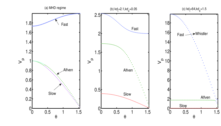
Figure 2: (a) Linear waves in MHD regime. Forward propagating fast, slow, and Alfvénic modes are shown. The top curve describes Alfvénic mode, whereas the remaining two curves are overlapped and represent fast and slow modes. Our results are consistent with Ref [[11]]. (b) High frequency waves in $kd_{i}>1$ and $kd_{e}<1$ (c) $kd_{i}>1$ and $kd_{e}>1$ regimes. It is clear from (b) and (c) that the propagation characteristic is modified dramatically in the short scale regimes. The phase speed increase for shorter scales. The parallel propagation is faster than the oblique one.

As a first step, we verify the consistency of our equation by comparing it with the MHD waves [11]. For this purpose, we use $d_{i}=d_{e}=0$ that reduces the dispersion relation to the usual compressible MHD relation. We retrieve MHD waves that are consistent with Ref [11]. This is shown in Fig (1a) that describes a phase velocity variation of the MHD waves as a function of angle between the propagation wave vector and the mean magnetic field, i.e. $k_{\parallel}=k\cos\theta$ where $k_{\parallel}={\bf k}\cdot{\bf B}_{0}$. We find three forward propagating modes with positive phase velocity that co-exist with three backward propagating modes with negative phase velocity. It is noteworthy that the shear Alfvén and slow modes are partially overlapped. In this regime, linear dynamics is entirely governed by the magnetosonic waves which is shown by the top curve in Fig (1a). A pure magnetic perturbation propagating orthogonal to the constant magnetic field in this regime behaves electrostatically and tends to move as a magnetosonic mode.

We next investigate the effect of a finite plasma beta on the propagation of the small scale magnetized waves to explore their dynamics in regimes III and IV in Fig (1). We choose parameters $\beta=3,k=0.5,d_{e}=0.1,d_{i}=43d_{e}$ that are characterize the high frequency modes between regions II and III. Since this parameter regime is not drastically different than the typical MHD regime, a non trivial modification in the dispersion of MHD waves is expected. For instance, the linear dynamics in this regime is governed predominantly by the higher frequency and short scale waves, namely kinetic Alfvén and magnetosonic waves. The density perturbation becomes significant in this regime. The dispersion of high frequency kinetic Alfvén, shown in Fig (2b), differs significantly from that in Fig (2a). The phase velocity of the kinetic Alfvén waves is increased, while the obliquely propagating kinetic Alfvén modes continue to remain unaffected. The shear Alfvén/slow modes decouple clearly. The fast modes travel with higher phase speed, whereas the slow modes propagate slower (than in Fig 2a). It is further clear from Fig (2b) that the propagation of the fast/slow modes depends crucially on the alignment of their wave vector relative the mean magnetic field. For a highly oblique propagation, these waves hardly move. Figure (2c) describes a regime where $kd_{i}>1$ and $kd_{e}\geq 1$. This is a regime where MHD modes are drastically altered and low frequency whistler modes start to play critical role. Shown in Fig (2c), the top curve is the whistler branch that survives whereas the bottom curves are reminiscent of MHD modes (Alfvén and fast/slow). As seen in Fig (2c), the whistler modes have higher frequency and phase speeds. They propagate predominantly along the field lines, whereas oblique whistlers have smaller phase speeds. At an angle $\theta=\pi/2$, the whistler modes do not propagate. They are transformed into high frequency electrostatic modes. Figure (2c) describes waves that possess length scales smaller than the ion inertial length, but bigger than electron inertial length scale. We can retrieve the small scale waves by choosing the small characteristic length scales of these waves relative to the ion inertial and electron inertial length scales. This is shown in Fig (3). This figure is further consistent with Fig (2) where the dynamics of small scale is described by choosing a relatively small magnitude of $k$ compared to $d_{i}$ and $d_{e}$ lengths.

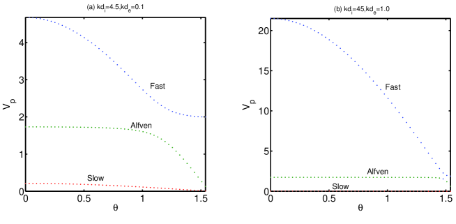
Figure 3: Figures (a) and (b) are shown for a large $k$. Note that the phase velocity of the small scale wave is consistent with Fig (2).

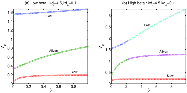
Figure 4: Effect of plasma beta is shown for large scale waves. (a) describes a low plasma beta regime, whereas (b) represents the higher beta regime.

4 Effect of plasma beta on the dispersive waves

We next investigate effect of plasma beta (ratio of plasma pressure and magnetic energy) on the propagation of dispersive waves in the solar wind plasma. We keep the angle of propagation constant ($\theta\simeq 45^{\circ}$) and vary plasma $\beta$ and study the waves corresponding to the small and large scale modes. A snap shot for the large scale waves is shown in Fig (4) that depicts effects of low (Fig 4a) and high (Fig 4b) plasma beta on the propagating waves. We find that the large scale Alfvén and slow waves continue to remain unaffected with regard to the beta varation. The propagation speed of the fast waves appears to grow linearly with the plasma beta. Hence there is a dramatic speed enhancement occurs for the fast waves. This is shown in Fig (4b).

Interestingly, we find that the propagation property of the dispersive waves corresponding to the small scale modes does not depend critically on the plasma beta. Almost all of these small scale waves remain unaffected relative to the beta variation. This is shown in Fig (5a) for the low beta regime, whereas Fig (5b) describes the effect of high plasma beta on the small scale dispersive waves.

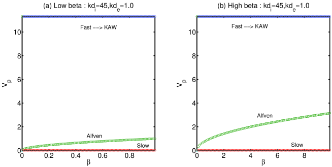
Figure 5: Phase speed variation with respect plasma beta for small scale dispersive waves. (a) and (b) describe respectively low and high beta regimes.

5 Summary

A major outcome of work is the inclusion of electron and ion inertia in strongly magnetized waves associated with a high beta plasma. We invoked a two fluid or Hall MHD model to examine the dynamics of these high frequency and fast time scale processes. We see that for the length scales $kd_{e}\geq 1$, where there the turbulent spectra shows a different power law behavior, the linear waves are significantly modified. It is clear from our work that the evolution of the linear waves in the MHD regime is modifed significantly in the dissipative or dispersive regime where $kd_{e}>kd_{i}>1$. This is the regime where solar wind turbulence is affected non trivially by the linear collision less waves. We find from our linear theory that MHD modes, such as Alfvén and fast/slow waves, are inconsequential in the small scale $kd_{e}>kd_{i}>1$ regime. This is because the MHD modes are relatively large scale and low frequency modes in comparison with the kinetic Alfvén and/or whistler modes that are typically excited in the $kd_{e}>kd_{i}>1$ regimes of Fig (1). Because of the great disparity in the length and time scales, the waves in the two distinct regimes (i.e. regimes III, IV and V in Fig 1) do not couple efficiently. Consequently, the linear dynamics of modes in the regimes IV and V is governed predominantly by fast and whistler modes respectively. The latter have a greater phase velocity relative to the MHD modes. Our results are important particularly to understand linear waves in the solar wind turbulence in the regime where small scale fluctuations exhibit dispersive characteristics [[1, 2, 4, 6, 5, 8, 9, 10]].

6 Acknowledgment

This research was partially supported by the NASA(NNX-08AE41G) NASA(NNG-05GH38) and NSF (ATM-0317509) grants.

19

References

- [1] Goldstein, M. L., Roberts, D. A., andMatthaeus, W. H. 1995 Magnetohydrodynamic turbulence in the solar wind, Ann. Rev. Astron. & Astrophys., 33 283.
- [2] Matthaeus, W. H., Goldstein, M. L., and King, J. H. 1986 An interplanetary magnetic field ensemble at 1 AU, J. Geophys. Res. 91, 59.
- [3] Goldstein, M. L., Roberts, D. A., and Fitch, C. A. 1994 Properties of the fluctuating magnetic helicity in the inertial and dissipation ranges of solar wind turbulence, J. Geophys. Res., 99 ,11519.
- [4] Leamon, R. J., Smith, C. W., Ness, N. F.,Matthaeus, W. H., and Wong K. Hung 1998 Observational constraints on the dynamics of the interplanetary magnetic field dissipation range, J. Geophys. Res., 103, 4775, .
- [5] Shaikh, D., and Zank, G. P. 2009 Spectral features of solar wind turbulent plasma, MNRAS, 15579.x 1365 DOI: 10.1111/j.
- [6] Smith, C. W., Matthaeus, W. H., and Ness, N. F. 1990 Proc. 21st Int. Conf. Cosmic Rays, 5. 280.
- [7] Biskamp, D., E. Schwarz, and Drake, J. F. 1996 Two-dimensional electron magnetohydrodynamic turbulence, Phys. Rev. Letts., 76, 1264.
- [8] Shaikh, D., and Zank, G. P. 2003 Anisotropic turbulence in two-dimensional electron magnetohydrodynamics, Astrophys. J. 599, 715 .
- [9] Shaikh, D. 2004 Generation of coherent structures in electron magnetohydrodynamics, Physica Scripta, 69, 216.
- [10] Shaikh, D., and Zank, G. P. 2005 Driven dissipative whistler wave turbulence, Phys. Plasmas 12, 122310.
- [11] Gurnet, D and Bhattacharjee, A. 2005 Introduction to Plasma Physics with Space and Laboratory applicatiom Oxford University Press.
- [12] Ishida, A., Cheng C. Z., and Peng, Y-K. M. 2005 Phys. Plasmas, 12 052113
- [13] Stringer, T. E. 1963 Low-frequency waves in an unbounded plasma, J. Nucl. Energy, Part C 5 89
- [14] Damiano, P. A., Wright, A. N. and McKenzie, J. F. 2009 Phys. Plasmas, 16, 062901
- [15] Swanson, D. G. 1989 Plasma Waves (Academic Press) Chapter 2
- [16] Shukla, P. K. 1978 Modulational instability of whistler-mode signals, Nature, 274, 874.
- [17] Shaikh, D., and Shukla, P. K. 2009 3D fluctuation spectra in the Hall-MHD plasma, Phys. Rev. Letts, 102, 045004.
- [18] Shukla, P. K., and Stenflo, L. 1985 Nonlinear propagation of electromagnetic Alfvén waves in a magnetoplasma, Phys. Fluids, 28, 1578.