Dynamics of thermalisation in small Hubbard-model systems

Abstract

We study numerically the thermalisation and temporal evolution of a two-site subsystem of a fermionic Hubbard model prepared far from equilibrium at a definite energy. Even for very small systems near quantum degeneracy, the subsystem can reach a steady state resembling equilibrium. This occurs for a non-perturbative coupling between the subsystem and the rest of the lattice where relaxation to equilibrium is Gaussian in time, in sharp contrast to perturbative results. We find similar results for random couplings, suggesting such behaviour is generic for small systems.

Understanding the origin of statistical mechanics from a purely quantum-mechanical description is an interesting area of active research canontyp ; popescu1 ; numerics_Jensen1985 ; *numerics_Saito1996; numerics_Henrich2005 ; numerics_yuan2009 ; rigol2008 ; *rigol2007; tasaki ; reimann ; srednicki1 . Of particular interest is the situation of an isolated quantum system partitioned into a subsystem and a bath. We ask the question: how do observables on the subsystem thermalise when the total system is in a pure state? Seminal works canontyp ; popescu1 have demonstrated the concept of ‘canonical typicality’ that most random pure states of well-defined energy for the total system lead to thermalised reduced density matrices (RDMs) for the small subsystem. Numerical works have demonstrated thermalisation in spin or boson systems for various observables of the subsystem numerics_Jensen1985 ; *numerics_Saito1996; numerics_Henrich2005 ; numerics_yuan2009 (and of the entire closed system rigol2008 ; *rigol2007; brody_ergodic2007 ; *fine2009). Recent theoretical work popescu2 has investigated whether thermalisation of small subsystems, initially far from equilibrium, is generic.

In this letter, we investigate the temporal relaxation towards a steady state, focusing on the regime where the steady state appears thermalised. We consider a small Hubbard ring of fermions away from half filling, with two adjacent sites as a subsystem and the other sites as a bath. We prepare the system in a product state of subsystem and bath pure states in a narrow energy window. Even for such a small system, we find a steady-state RDM close to a thermal state, down to quantum degenerate temperatures. Moreover, we find that the RDM diagonal elements approach a steady state as an exponential decay for weak subsystem-bath coupling. This becomes a Gaussian decay at a non-perturbative coupling, with a decay rate that departs significantly from the Fermi golden rule. We note that this is distinct from the Gaussian behaviour in driven systems that remain out of equilibrium segal2007 , and in decoherence dynamics rossini2007 ; *cucchietti2007; *dobrovitski2008; *numerics_yuan2008 of off-diagonal RDM elements in systems that cannot thermalise.

The Model. Taking motivation from cold atoms in optical lattices sherson2010 ; bakr2010 where local addressing is possible, we study a local cluster in a generic (non-integrable) interacting system with a quasi-continuous spectrum. We will examine how a local subsystem ($S$) thermalises with the rest of the system as a bath ($B$) via unitary evolution of the whole system under the Hamiltonian ${H}={H}_{S}+{H}_{B}+\lambda{V}$ where ${H}_{S}$ (${H}_{B}$), with eigenstates $|s\rangle_{S}$ ($|b\rangle_{B}$) of energy $\varepsilon_{s}$ ($\epsilon_{b}$), acts solely on the subsystem (bath). $\lambda V$ is the coupling between the subsystem and the bath. For $\lambda=0$, the eigenstates are products of subsystem and bath eigenstates, denoted $|sb\rangle$, with energies $E_{sb}=\varepsilon_{s}+\epsilon_{b}$. The homogeneous case corresponds to $\lambda=1$. Specifically, we choose a two-site subsystem in an $L$-site Hubbard ring of fermions:

$${H}_{S} = -\sum_{\sigma=\uparrow,\downarrow}J_{\sigma}(c^{\dagger}_{1\sigma}c_{2\sigma}+\text{h.c.})+U(n_{1\uparrow}n_{1\downarrow}+n_{2\uparrow}n_{2\downarrow})\,,$$

$${H}_{B} = -\sum_{i=3}^{L-1}\sum_{\sigma=\uparrow,\downarrow}J_{\sigma}(c^{\dagger}_{i\sigma}c_{i+1,\sigma}+\text{h.c.})+U\sum_{i=3}^{L}n_{i\uparrow}n_{i\downarrow}\,,$$

$${V} = -\sum_{\sigma=\uparrow,\downarrow}J_{\sigma}\left[(c_{2\sigma}^{\dagger}c_{3\sigma}+c_{1\sigma}^{\dagger}c_{L\sigma})+\text{h.c.}\right]\,,$$ (1)

where $n_{i\sigma}=c^{\dagger}_{i\sigma}c_{i\sigma}$ is the number operator on site $i$ with spin $\sigma$. The lattice is a ring with the subsystem sites at $i=1,2$ and bath sites at $i=3$ to $L$. The hopping integrals are $J_{\sigma}=J(1+\xi\;\text{sgn}(\sigma))$, with a non-zero $\xi=0.05$ to remove level degeneracies due to spin rotation symmetry. We set the on-site repulsion $U=J$ to give us a metallic system with interacting bath modes while avoiding the formation of strong features in the many-body density of states at $U\gg J$ arising from Hubbard interactions. We will let $J$ be the unit of energy. This Hamiltonian preserves the total particle number, $N$, and spin component, $S^{z}$, but not the total spin $S^{2}$. In this work, we fill the $L=9$ lattice with 8 fermions of total spin $S^{z}=0$. The two-site subsystem has 16 eigenstates and the bath has 8281 eigenstates, while the composite system has a total of 15876 states with average level spacing $\Delta\simeq 10^{-3}$. This is small enough to allow exact diagonalisation, but large enough to provide a smooth density of states.

Consider a system prepared in a pure state of the form

$$|\Psi(t=0),E_{0}\rangle=\sum_{b_{i}=b_{l}}^{b_{u}}\frac{1}{\sqrt{B}}|s_{i}b_{i}\rangle$$ (2)

where $|s_{i}\rangle_{S}$ is the initial subsystem state, e.g. $|\!\uparrow,\uparrow\rangle_{S}$ with parallel spins on the two sites. $|\Psi(t=0)\rangle$ contains a linear combination of $B$ bath eigenstates $|b_{i}\rangle_{B}$ within an energy shell of width $\delta_{B}$, chosen such that $\langle\Psi|H|\Psi\rangle=E_{0}$. The width $\delta_{B}$ (= 0.5 in this work) is small on the scale for variations in the density of states. The system evolves in time: $|\Psi(t)\rangle=e^{-iHt}|\Psi(0)\rangle$. The subsystem is described completely by the RDM which traces over the bath states $|b\rangle_{B}$: $\rho(t)=\text{Tr}_{B}|\Psi(t)\rangle\langle\Psi(t)|$. This is evaluated using the eigenstates of $H$ from exact diagonalisation.

Equilibrium States. Before discussing relaxation dynamics during thermalisation, we identify first the parameter regime where $\rho$ does relax to thermal equilibrium. We say that a subsystem thermalises if its RDM $\rho(t)$ approaches the thermal RDM $\omega$ after some time $t$ (shorter than $\Delta^{-1}$.) The thermal RDM, $\omega$, is diagonal with elements $\omega_{ss}={}_{S}\langle s|\omega|s\rangle_{S}\propto N_{B}(E_{0}-\varepsilon_{s},N-n_{s},S^{z}-s^{z}_{s})$, where $|s\rangle_{S}$ is a subsystem eigenstate $|s\rangle_{S}$ with energy $\varepsilon_{s}$, $n_{s}$ particles and spin $s_{s}^{z}$ and $N_{B}(E,n_{b},s^{z}_{b})$ is the number of bath states with energies in $[E,E+\delta E]$ with $n_{b}$ particles and spin $s^{z}_{b}$. We have to specify energy, number and spin because they are globally conserved by the Hamiltonian $H$. We can define an effective temperature $T_{\text{eff}}=[\partial\log N_{B}/\partial E|_{E_{0}}]^{-1}$ provided that the system is in a state with energy uncertainty $\delta E\gg\Delta$, the level spacing. (In the thermodynamic limit, $\omega$ takes the form of a Gibbs canonical distribution brody_ergodic2007 ; *fine2009 — if particles are not exchanged with the bath, $\omega_{ss}\propto e^{-\varepsilon_{s}/T}$.)

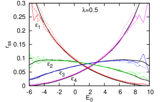
Figure 1: (Colour online) Time average of diagonal RDM elements, $r_{ss}$, for the $n_{s}=2$, $s^{z}_{s}=0$ sector as a function of composite energy $E_{0}$, for initial subsystem states $|\!\uparrow\downarrow,\uparrow\rangle_{S}$ (solid line), $|\!\uparrow,\uparrow\rangle_{S}$ (dashed) and $|\!\uparrow,\downarrow\rangle_{S}$ (dotted). The four elements are labelled by their energies, ascending from $\varepsilon_{1}$ to $\varepsilon_{4}$. Thick lines: the corresponding elements for the thermal state $\omega$, found by counting bath states with spin $S^{z}-s^{z}_{s}$ and $N-n_{s}$ particles within a Gaussian energy window of width $\delta E=0.5$, centered on energy $E_{0}-\varepsilon_{s}$.

We now present our results for a system starting from the initial states (2). We avoid the regime of very small subsystem-bath coupling $\lambda$ where the subsystem RDM, $\rho$, is strongly dependent on the initial state even at long times due to finite-size effects. Nevertheless, we find that even such a small system can reach a steady state for couplings $\lambda$ larger than a surprisingly small crossover value $\lambda_{\rm th}\ll 1$. The RDM becomes virtually diagonal — even the sum over the fluctuating off-diagonal elements, $[\sum_{s\neq s^{\prime}}r_{ss^{\prime}}^{2}]^{1/2}$, is 10^-1 to 10^-3 smaller than each diagonal element. Fig. 1 shows the steady-state values of the diagonal elements of the RDM, $r=\lim_{\tau\rightarrow\infty}\int_{0}^{\tau}\rho(t)dt/\tau$ as a function of the composite energy $E_{0}$ for a coupling of $\lambda=0.5$. For a variety of initial states, $\rho(t)$ is only weakly dependent on the details of the initial state at long times for $-3\apprle E_{0}\apprle 6$, approaching the thermal form $\omega$ expected from the canonical ensemble.

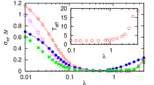
Figure 2: Dependence on the initial state, $\Delta r$ (solid), and distance from the thermal state, $\sigma_{\omega}$ (hollow), as a function of coupling $\lambda$, at composite energies $E_{0}=-2$ (circle) and $1.77$ (square). Inset: effective temperature $T_{\text{eff}}$ for $E_{0}=-2$.

Next, we establish the range of the coupling $\lambda$ over which the system forgets its initial state and thermalises. We expect the system to retain memory of the initial state at weak coupling ($\lambda\ll 1$). Moreover, for $\lambda\gg 1$, the eigenspectrum becomes significantly altered by the coupling, splitting into several bands and we see oscillations. This is a feature of the projection of the initial state on the strongly-coupled link. Therefore, we expect that the loss of memory of the initial state and thermalisation are possible only in a range of intermediate couplings. To quantify this, we calculated the root-mean-square variation in diagonal RDM elements due to using different initial subsystem states: $\Delta r=\frac{1}{2}\sum_{s}[{\langle{r_{ss}}^{2}\rangle-\langle{r_{ss}}\rangle^{2}}]^{\frac{1}{2}}$, with $\langle\ldots\rangle$ averaging over all $16$ initial states in the subsystem Fock basis (i.e., eigenstates at $J=0$). A small $\Delta r$ indicates memory loss. We have also measured the closeness to the thermal state $\omega$ using $\sigma_{\omega}=\frac{1}{2}\sum_{s}\langle\left|{r_{ss}}-\omega_{ss}\right|\rangle$. We see from Fig. 2 that memory loss and thermalisation occur in the intermediate range $\lambda_{\rm th}\apprle\lambda\apprle 3$ with crossover value $\lambda_{\rm th}\simeq 0.1$ at $E_{0}=-2$ and $1.77$.

We also find that the relative probabilities of different states in the $n_{s}=2$, $s^{z}_{s}=0$ sector fit a Boltzmann form: $\log r_{ss}=-\varepsilon_{s}/T_{\text{eff}}+\text{const}$. For states near the centre of the eigenspectrum ($E_{0}\simeq 1.77$), the effective temperature $T_{\text{eff}}$ is infinite. At $E_{0}=-2$, we find $T_{\text{eff}}\simeq 2$ up to $\lambda\sim 2$ (Fig. 2 inset). We estimate the chemical potential to be $2J\simeq 2$ so that, unlike in previous work, we see thermalisation at temperatures down to quantum degeneracy.

We note that these thermalised systems are surprisingly small. Popescu et al. popescu1 give an estimate of the number $d_{R}$ of composite-system eigenstates spanned by the initial state sufficient for thermalisation — if the probability that $\sigma_{\omega}>Y=0.1$ is at least as small as $X=0.01$, then $d_{R}>(9\pi^{3}/2Y^{2})\ln(2/X)\simeq 70000$. This is almost two orders of magnitude larger than the number of states ($\gtrsim\delta_{B}/\Delta$) spanned by our initial state which is as low as 950. Moreover, we find thermalisation at $U=J$ for smaller systems than at $U\ll J$. We believe strong inelastic scattering in the interacting bath enables efficient thermalisation at $U=J$ when system size is larger than the inelastic scattering length ($\propto J^{2}/U^{2}$ for small $U/J$).

Time Evolution. Having established the coupling range for thermalisation for model (1), we will now discuss our main results for the temporal relaxation towards the steady state. Fig. 3 shows examples of the time evolution of the diagonal RDM element $\rho_{ss}(t)$ with $s=s_{i}$ for two coupling strengths. The system is again prepared in the product state (2) with $|s_{i}\rangle_{S}=|\!\uparrow,\uparrow\rangle_{S}$. These results are computed for energy $E_{0}=-2$. We do not expect our results to depend strongly on $E_{0}$ unless the system is close to a strongly correlated ground state.

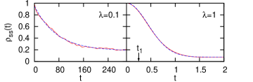
Figure 3: The RDM element $\rho_{ss}$ as a function of time $t$ with $s=|\!\uparrow,\uparrow\rangle$ for the initial state (2) at total energy $E_{0}=-2$ ($T_{\text{eff}}\simeq 2$) with $s_{i}=s$. Left: coupling $\lambda=0.1$ with exponential fit (dashed). Right: $\lambda=1$ with Gaussian fit (dashed).

We find qualitatively different relaxation behaviour for perturbative and non-perturbative couplings (Fig. 3). Whereas the RDM relaxes towards the steady state exponentially in time at weak coupling ($\lambda<\lambda_{\rm exp}$), the relaxation follows a Gaussian form at larger coupling ($\lambda>\lambda_{\rm Gauss}$). Interestingly, this Gaussian regime covers the coupling range where the system thermalises.

We can understand our results at short times or weak coupling. At short times, we can approximate $|\Psi(t)\rangle\simeq(1-iHt)|\Psi(0)\rangle$. It can be shown (and our numerics agree) that the element $\rho_{s_{i}s_{i}}(t)\simeq 1-\Gamma_{1}^{2}t^{2}$ for $t<t_{1}=1/\max(E_{sb}-E_{0})$, with $\Gamma_{1}=\lambda[\sum_{s\neq s_{i},b}|\langle sb|V|\Psi(0)\rangle|^{2}]^{1/2}$. The maximum energy difference between states coupled by hopping ($V$) is of the order of the single-particle bandwidth $4J$ and so $t_{1}\simeq 1/4$.

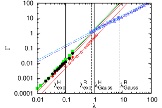
Figure 4: (Colour online) Rates of decay of $\rho_{s_{i}s_{i}}$ for the subsystem state $s_{i}=|\!\uparrow,\uparrow\rangle$ with initial state (2) at $E_{0}=-2$ ($\CIRCLE$/$+$) and 1.77 ($\blacksquare$/$\times$) and random model at $E_{0}=-2$ ($\Circle$/$\triangle$). Weak coupling/exponential decay: $-d\rho_{s_{i}s_{i}}/dt|_{t=0}$ at short times found from exponential fits ($\CIRCLE$,$\blacksquare$,$\Circle$) agree with Fermi golden rule prediction, $\gamma_{\rm FGR}$ (solid lines, gradient 2). Moderate coupling/Gaussian decay: fit to Gaussian with rate $\Gamma$ ($\times$,$+$,$\triangle$) agrees with $\Gamma_{1}$ (dashed lines, gradient 1). Vertical lines mark estimates of the crossover values $\lambda_{\rm exp}$ and $\lambda_{\rm Gauss}$ ($\lambda^{\text{H/R}}$ for Hubbard/random models). Data in the crossover region are rates obtained from attempted fits to either form.

At weak coupling, we can go beyond $t_{1}$ by treating the coupling $\lambda V$ as a perturbation to the uncoupled Hamiltonian $H_{S}+H_{B}$. It is readily shown that, to leading order in $\lambda$, the RDM element corresponding to a subsystem state $s\neq s_{i}$ is approximated by $\tilde{\rho}(t)$:

$$\tilde{\rho}_{ss}(t)\!=\!\frac{4\lambda^{2}}{B}\!\sum_{b}\!\left|\sum_{b_{i}=b_{l}}^{b_{u}}\!\frac{\sin[(E_{sb}\!-\!E_{s_{i}b_{i}})\frac{t}{2}]}{E_{sb}-E_{s_{i}b_{i}}}\langle sb|V|s_{i}b_{i}\rangle\right|^{2}$$ (3)

after the composite system is prepared in the state (2). The element $\tilde{\rho}_{s_{i}s_{i}}$ is most readily found by using $\text{Tr}(\tilde{\rho})=1$ to give $\tilde{\rho}_{s_{i}s_{i}}(t)=1-\sum_{s\neq s_{i}}\tilde{\rho}_{ss}(t)$. This perturbation theory is valid until time $t_{2}$ when $\rho_{s_{i}s_{i}}$ has dropped significantly below unity. For times between $t_{1}$ and $t_{2}$, eq. (3) follows the Fermi golden rule (FGR): $\rho_{s_{i}s_{i}}(t)$ decreases linearly in time with $d\rho_{s_{i}s_{i}}/dt\propto-\lambda^{2}$. Beyond the FGR regime, we expect to see exponential decay (see, e.g., approximate Markovian schemes of the Lindblad type BreuerPetruccione ) as is found in our data (Fig. 3 left) for $\lambda\apprle\lambda_{\rm exp}=0.1$. In our case, the initial state is not a bath eigenstate. This gives small fluctuations on top of a simple linear-$t$ decay, due to interference between terms in the inner sum in (3).

We check in Fig. 4 that the FGR prediction agrees quantitatively with $d\rho_{s_{i}s_{i}}/dt|_{t=0}$ for $E_{0}=-2$ and $1.77$, found from the parameters obtained for the exponential fit to $\rho_{s_{i}s_{i}}$ for $t>t_{1}$: $\rho_{s_{i}s_{i}}(t)\sim Ae^{-(t-t_{0})/\tau}+(1-A)$. The FGR rate, $\gamma_{\rm FGR}$, is found by averaging (3) over a time $t$ between $t_{1}$ and $t_{2}$: $-\gamma_{\rm FGR}t=\int_{0}^{t}[\tilde{\rho}_{s_{i}s_{i}}(t^{\prime})-1]dt^{\prime}/t$. This procedure is needed for a non-zero level spacing $\Delta$. We point out that the exponential fit fails at very weak coupling ($\lambda\sim 10^{-2}$) when the system barely relaxes.

We now consider larger couplings where $\lambda\sim O(1)$. Instead of exponential relaxation, we find a good fit (Fig. 3 right) to a Gaussian decay: $\rho_{s_{i}s_{i}}(t)\sim Ce^{-\Gamma^{2}t^{2}}+(1-C)$. This is seen for couplings $\lambda\apprge\lambda_{\rm Gauss}=1$. The decay rate $\Gamma$ now increases linearly with $\lambda$ and is as large as the bandwidth scale $1/t_{1}\simeq 4$. It appears insensitive to energy $E_{0}$. Interestingly, we see in Fig 4 that, in the regime where $\Gamma t_{1}\sim 1$, the decay rate $\Gamma$ is well approximated by $\Gamma_{1}$ from the short-time expansion, which suggests $\Gamma=\Gamma_{1}/C^{\frac{1}{2}}$. (In our data, $0.97<C^{\frac{1}{2}}<1$.) In other words, perturbation theory gives the early-time precursor to the full Gaussian form. This suggests the interpretation that the time interval of validity of the Fermi golden rule ($t_{1}<t<t_{2}$) narrows and vanishes as $\lambda$ increases to $\lambda_{\rm Gauss}$. For coupling range $\lambda_{\rm exp}<\lambda<\lambda_{\rm Gauss}$, the behaviour is less clear cut — the decay starts as a Gaussian but becomes exponential at later times. The amplitude of this exponential tail decreases with increasing $\lambda$, becoming negligible as $\lambda$ reaches $\lambda_{\rm Gauss}$.

Random Couplings. To verify that the two regimes of relaxation are not specific to our model Hamiltonian, we proceeded to study an alternative model where the subsystem-bath coupling $V$ is replaced by a random Hermitian matrix $W$ which still respects the conservation of the global particle number $N$ and spin $S^{z}$. Each non-zero matrix element of $W$ is Gaussian distributed, with the variance chosen such that $\text{Tr}(W^{2})=\text{Tr}(V^{2})$. Thus, we can compare $H=H_{S}+H_{B}+\lambda V$ with $H=H_{S}+H_{B}+\lambda W$ with similar decay rates. In this model, we expect $1/t_{1}$ to be of the order of the full bandwidth $\sim 20$ for $N=8$, $S^{z}=0$. We find exponential relaxation at weak coupling, $\lambda\apprle\lambda_{\rm exp}=0.8$, and we recover Gaussian relaxation with a linear-$\lambda$ decay rate for $\lambda\apprge\lambda_{\rm Gauss}=8$ (Fig. 4, hollow symbols). The crossover values, $\lambda_{\rm exp}$ and $\lambda_{\rm Gauss}$, occur at nominally higher couplings than for the Hubbard ring (1). They become closer to the Hubbard-ring values if we mimic the structure of $V$ by restricting the states coupled by $W$: $\langle s^{\prime}b^{\prime}|W|sb\rangle\neq 0$ only if $|E_{s^{\prime}b^{\prime}}-E_{sb}|<4J$, the single-particle bandwidth.

We summarise our results in Fig. 5. We have shown that a two-site subsystem of the Hubbard model relaxes to steady states resembling canonical thermal states, even for systems with a handful of sites and at quantum degenerate energies. This occurs at a non-perturbative coupling between the subsystem and bath, corresponding to nearly homogeneous systems. In this regime, the reduced density matrix $\rho(t)$ displays Gaussian relaxation to the thermal state, with a decay rate $\Gamma$ linear in the coupling $\lambda$. This contrasts sharply with the perturbative regime where $\rho(t)$ exhibits an exponential relaxation with a $\lambda^{2}$ decay rate. We believe that the Gaussian relaxation to thermalisation is a generic feature of closed nanoscale systems, as is supported by our results for random Hamiltonians.

Finally, we note that it can be shown that $\Gamma_{1}t_{1}\sim\lambda Jt_{1}\sim\lambda$ irrespective of system size. The subsystem thermalises on the time scale of a few hops between the subsystem and the bath, by inelastic collisions of the fermions within this timescale. This should be insensitive to system size for systems larger than the inelastic scattering length. Therefore, we speculate that the observed Gaussian relaxation should remain for large systems.

Figure 5: Schematic behaviour of the reduced density matrix $\rho(t)$ as a function of subsystem-bath coupling $\lambda$. Top: relaxation to steady state. Bottom: steady state of $\rho(t)$. Memory of initial state also occurs at large $\lambda$ in the Hubbard case.

We are grateful to Miguel Cazalilla for useful discussions. We wish to thank Imperial College HPC for computing resources as well as EPSRC for financial support.

References

- (1) S. Goldstein, J. L. Lebowitz, R. Tumulka, and N. Zanghì, Phys. Rev. Lett. 96, 050403 (Feb 2006)
- (2) S. Popescu, A. J. Short, and A. Winter, Nature Phys. 2, 754 (2006)
- (3) R. V. Jensen and R. Shankar, Phys. Rev. Lett. 54, 1879 (Apr 1985)
- (4) K. Saito, S. Takesue, and S. Miyashita, J. Phys. Soc. Jpn. 65, 1243 (1996)
- (5) M. J. Henrich, M. Michel, M. Hartmann, G. Mahler, and J. Gemmer, Phys. Rev. E 72, 026104 (Aug 2005)
- (6) S. Yuan, M. Katsnelson, and H. De Raedt, J. Phys. Soc. Jpn. 78, 094003 (2009)
- (7) M. Rigol, V. Dunjko, and M. Olshanii, Nature 452, 854 (2008)
- (8) M. Rigol, V. Dunjko, V. Yurovsky, and M. Olshanii, J. Phys. A 40, F503 (2007)
- (9) H. Tasaki, Phys. Rev. Lett. 80, 1373 (Feb 1998)
- (10) P. Reimann, Phys. Rev. Lett. 99, 160404 (Oct 2007)
- (11) M. Srednicki, J. Phys. A 29, L75 (1996)
- (12) D. C. Brody, D. W. Hook, and L. P. Hughston, J. Phys. A:Math. Theor. 40, F503 (2007)
- (13) B. V. Fine, Phys. Rev. E 80, 051130 (Nov 2009)
- (14) N. Linden, S. Popescu, A. J. Short, and A. Winter, Phys. Rev. E 79, 061103 (Jun 2009)
- (15) D. Segal, D. R. Reichman, and A. J. Millis, Phys. Rev. B 76, 195316 (Nov 2007)
- (16) D. Rossini, T. Calarco, V. Giovannetti, S. Montangero, and R. Fazio, Phys. Rev. A 75, 032333 (Mar 2007)
- (17) F. M. Cucchietti, S. Fernandez-Vidal, and J. P. Paz, Phys. Rev. A 75, 032337 (Mar 2007)
- (18) V. V. Dobrovitski, A. E. Feiguin, D. D. Awschalom, and R. Hanson, Phys. Rev. B 77, 245212 (Jun 2008)
- (19) S. Yuan, M. I. Katsnelson, and H. De Raedt, Phys. Rev. B 77, 184301 (May 2008)
- (20) J. F. Sherson, C. Weitenberg, M. Endres, M. Cheneau, I. Bloch, and S. Kuhr, Nature 467, 68 (2010)
- (21) W. S. Bakr, A. Peng, M. E. Tai, R. Ma, J. Simon, J. I. Gillen, S. Folling, L. Pollet, and M. Greiner, Science 329, 547 (2010)
- (22) M.-P. Breuer and F. Petruccione, The Theory of Open Quantum Systems (Oxford University Press, 2006)